Methods for the determination of the structures and dynamics of proteins by solid state NMR spectroscopy

warwick.ac.uk/lib-publications

A Thesis Submitted for the Degree of PhD at the University of Warwick

Permanent WRAP URL:

http://wrap.warwick.ac.uk/78994

Copyright and reuse:

This thesis is made available online and is protected by original copyright. Please scroll down to view the document itself.

Please refer to the repository record for this item for information to help you to cite it. Our policy information is available from the repository home page.

Methods for the Determination of the Structures and

Dynamics of Proteins by Solid-State NMR Spectroscopy

by

Jonathan Mark Lamley

Thesis

Submitted to the University of Warwick

for the degree of

Doctor of Philosophy

Supervised by Dr. Józef R. Lewandowski

Department of Chemistry

— i —

C

ONTENTS

List of Tables

vi

List of Figures

vi

Acknowledgements

x

Declarations

xi

Abstract

xii

Abbreviations

xiii

Chapter 1 – Introduction

1

Chapter 2 – Nuclear Magnetic Resonance Theory

7

2.1

Theoretical foundations of Magnetic Resonance...

7

2.1.1 The Zeeman Interaction

...

7

2.1.2 The Density Operator

...

9

2.1.3 Interaction Hamiltonians

...

10

2.1.4 Chemical Shielding

...

14

2.1.5 Dipolar Coupling

...

16

2.1.6 J-Coupling

...

18

2.1.7 Other Interaction

...

19

2.1.8 Magic Angle Spinning

...

20

2.2

The Pulsed-FT NMR Experiment...

22

2.2.1 The B1 Field

...

24

2.2.2 The NMR Signal

...

26

2.2.3 The Fourier Transform

...

28

2.2.4 Experimental Sensitivity

...

29

2.2.5 Cross-Polarisation

...

31

2.2.6 Decoupling

...

35

— ii —

2.2.8 Three-Dimensional Spectroscopy

...

40

2.2.9 Phase Cycling

...

40

2.3

Nuclear Relaxation...

41

2.3.1 Spin-Lattice (T1) Relaxation

...

41

2.3.2 Spin-Spin (T2) Relaxation

...

44

2.3.3 The Spectral Density Function

...

45

2.3.4 Semi-Classical Relaxation Theory

...

47

2.3.5 The T1 Relaxation Rate

...

49

2.3.6 The T2 Relaxation Rate

...

51

2.3.7 Spin-Lattice Relaxation in the Rotating Frame

...

52

Chapter 3 – SSNMR for Structural Studies of Proteins

56

3.1

Protein Samples for SSNMR...

56

3.2

Recoupling Techniques...

61

3.3

Spectral Assignment...

67

3.4

Structural Information...

69

3.5

Challenges and Progress...

71

Chapter 4 – Time-Shared Third Spin-Assisted Recoupling

73

4.1

Introduction...

73

4.2

Experimental Details...

75

4.3

Results and Discussion...

77

4.4

Conclusions...

81

Chapter 5 – SSNMR of a Protein in a Precipitated Complex

with a Full-Length Antibody

83

5.1

Introduction...

83

5.2

Results and Discussion ...

86

5.3

Conclusions...

97

— iii —

Chapter 6 –

_{H-Detected SSNMR Experiments at 80-100 kHz}

MAS

100

6.1

Introduction... 100

6.2

Evaluation of Line Widths...

102

6.3

Application to Small Molecules...

106

6.4

Application to Proteins...

107

6.5

Conclusions...

110

6.6

Experimental Details... 110

6.6.1 _β-L-Asp-L-Ala and Erythromycin Experiments

...

110

6.6.2 Protein Experiments

...

112

Chapter 7 – MAS-NMR Relaxation Methods for Characterising

the Dynamics of Proteins

113

7.1

Introduction... 113

7.2

Relaxation Methods... 115

7.3

Picosecond-Nanosecond Motions: Spin-Lattice Relaxation.... 116

7.4

Nanosecond-Millisecond Motions: Spin-Spin Relaxation and

Spin-Lattice Relaxation in the Rotating Frame...

118

7.5

Microsecond-Millisecond Exchange Processes: Relaxation

Dispersion...

120

7.6

Quantitative Analysis of Relaxation Rates...

121

Chapter 8 – Slow Protein Dynamics in Different Molecular

Environments: >300 kDa Complex versus Crystal

125

8.1

Introduction... 125

8.2

Results and Discussion...

126

8.3

Conclusions...

130

8.4

Experimental Details... 131

— iv —

9.2

Evaluation of Spin Diffusion Effects...

136

9.3

Measurement of

_C

_R

and R

Relaxation Rates...

141

9.4

Conclusions...

143

9.5

Experimental Details... 144

Chapter 10 – Protein Backbone Motions from Combined

_C’

and

_{N SSNMR Relaxation Measurements}

146

10.1 Introduction... 146

10.2 Evaluation of Coherent Contributions to

_{C’ R}

...

148

10.3 Measurement of

_{C’ and}

_{N R}

and R

Relaxation Rates... 151

10.4 Quantification of

_{C’ and}

_{N Relaxation Rates using the}

Simple Model-Free Approach...

154

10.5 Differences Between Results of SMF Analyses of

_{C’ and}

_{N Relaxation Rates...}

156

10.6 Extended Model-Free Analysis of Peptide Plane Motions...

161

10.7 Conclusions...

165

10.8 Experimental Details... 165

Chapter 11 – Summary and Outlook

167

Appendix A – Expressions for Quantum Mechanics

172

A.1 Spin Operators and Matrices...

172

A.2 Tensors and Rotations...

172

A.3 Chemical Shift...

173

A.4 Dipolar Coupling...

174

Appendix B – Supplementary Information for Structural

SSNMR Studies

175

B.1 Supplementary Figures for Chapter 4... 175

B.2 Amino Acid Sequence and Structure of the B1 Domain of

Protein G (GB1 – 56 Residues)...

177

B.3 Supplementary Figures for Chapter 5... 178

— v —

Appendix C – Supplementary Information for SSNMR

Dynamics Studies

C.1 Supplementary Figures for Chapter 8... 181

C.2 Supplementary Figures for Chapter 9... 187

C.3 Supplementary Figures for Chapter 10...

187

C.4 Evaluation of Robustness of

_{C’ R}

Experiments... 192

C.1.1 Magic Angle Mis-Adjustment

...

192

C.1.2 Temperature Effects

...

192

C.1.3 Polarisation Transfer

...

194

C.5 Details of Quantitative Analysis of Relaxation Data... 195

C.6 Solution-State Extended Model-Free Analysis...

196

— vi —

L

IST OF

T

ABLES

2.1 Properties of common nuclei in biological NMR……….. 30

6.1 1_{H line widths of β-Asp-Ala at 100 kHz MAS and 850 MHz} 1_{H Larmor} frequency……….. 105

C.1 Summary of relaxation-active interactions used for model-free analyses of GB1……….… 195

L

IST OF

F

IGURES

2.2 Euler angle rotations………... 13

2.3 Dipolar coupling………. 17

2.4 Magic angle spinning………... 21

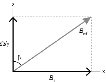
2.5 Effective B1 field………. 26

2.6 Absorptive and dispersive line shapes and truncation……….. 28

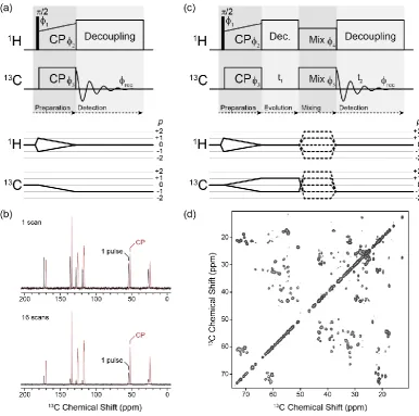
2.7 Pulse sequences, coherence pathways and example spectra for CP and two-dimensional experiments……….. 33

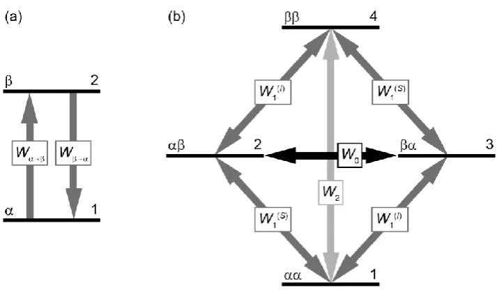
2.8 Energy level diagrams and transition rates for a single spin system and for a 2-spin system……….. 43

2.9 Correlation functions, spectral densities and R1 and R2 relaxation rates as a function of motional correlation time………... 46

3.1 13_{C enrichment pattern for amino acids expressed using [2-}13_{C]glycerol... 58}

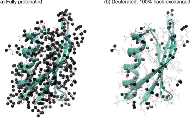
3.2 Effect of deuteration on the concentration of protons in a protein……. 59

3.3 Example spectra and pulse sequences for recoupling techniques: NCO, NCA, RFDR and 1_{H-detected inverse CP……….... 63}

3.4 Representation of a sequential assignment strategy……….. 68

4.1 TSTSAR pulse sequences……… 74

4.2 Numerical simulations of TSAR polarisation transfer in a NCα_Hα_Cβ_Hβ1_Hβ2 _{spin system……….... 77}

4.3 Broadband 2D PAR and TSTSAR spectra of [U-13_C,15_{N]histidine……... 78}

4.4 Aliphatic 2D PAR and TSTSAR spectra of [U-13_C,15_{N]-N-Acetyl-L} -Val-L-Leu………... 79

— vii —

5.1 2D 15_N-1_{H spectra of deuterated (100% back-exchanged) GB1 in}

complex with IgG, with and without CuII_{-EDTA at 60 kHz MAS…….. 86}

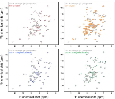
5.2 Overlays of 2D 15_N-1_{H spectrum of precipitated deuterated GB1-IgG}

complex with equivalent spectra of GB1 in solution, crystalline GB1, GB1-Fc fragment complex in solution and GB2-Fab fragment complex

in solution………... 88 5.3 Representative strips from 3D H(H)NH, CONH and CO(CA)NH

spectra on deuterated GB1-IgG complex……… 89 5.4 Representative planes from 3D NCAH spectrum on deuterated

GB1-IgG complex………... 89 5.5 Representative slices (1_{H dimension) from 3D CONH, CO(CA)NH}

and CANH spectra on deuterated GB1-IgG complex………. 90 5.6 Assigned 2D 15_N-1_{H spectrum of deuterated GB1-IgG complex………. 90}

5.7 Chemical shift perturbations for precipitated GB1-IgG complex and

GB1 in solution………... 91 5.8 15_N-1_{H spectrum of precipitated GB1-IgG complex with, for interacting}

residues, peaks indicated for GB1-Fc fragment complex in solution and

GB1 in solution………... 92 5.9 15_N-1_{H spectrum of precipitated GB1-IgG complex with, for interacting}

residues, peaks indicated for GB2-Fab fragment complex in solution

and GB1 in solution……… 93 5.10 Expansions, for example interacting residues, of the 15_N-1_{H spectrum of}

precipitated GB1-IgG complex, with peaks indicated for GB1, GB1-Fc

and GB1-Fab in solution………. 94 5.11 Secondary Cα _{chemical shifts for GB1 in solution and for precipitated}

GB1-IgG complex………... 95 5.12 Signal to noise ratios of peaks in Figure 5.6………. 96

6.1 1D 1_{H spectrum of β-Asp-Ala as a function of MAS frequency……….. 103}

6.2 Total and homogeneous 1_{H line widths of β-Asp-Ala as a function of}

inverse MAS frequency……….... 104 6.3 2D 13_C-1_{H spectra of β-Asp-Ala and erythromycin……….. 107}

6.4 2D 15_N-1_{H spectra of deuterated GB1-IgG complex, with and without}

CuII_{-EDTA, and of protonated GB1-IgG complex, at 95-100 kHz MAS 108}

7.1 Time scales of dynamic processes in proteins and NMR dynamic probes 114 7.2 Illustration of spin diffusion;13_{C’ R}

1 relaxation rates measured in

[U-13_C,15_{N]Ala at 16.1 kHz and 60.0 kHz MAS………. 117}

7.3 Illustration of coherent contributions to measured R1ρ decay rates; 15N

R₁ρ relaxation rates measured in [U-13C,15N]GB1 as a function of

spinning frequency and of spin-lock nutation frequency……….. 118 7.4 Order parameters and correlation times from SMF analysis of 15_N

— viii — 8.1 15_{N R}

1ρ relaxation measurements in deuterated GB1-IgG complex and

in deuterated (100%back-exchanged) crystalline GB1……… 127

8.2 15_{N R} 1ρ relaxation rates projected onto structure of GB1, for GB1-IgG complex and for crystalline GB1………. 128

8.3 Residues of GB1 undergoing chemical exchange in GB1-IgG complex and in crystal………... 129

9.1 Expansions from 2D 13_C-1_{H spectra of fully protonated [U-}13_C,15_N]GB1 at 60 kHz MAS and 14.1 T, and of [1,3-13_C,15_{N]GB1 at 100 kHz MAS} and 20.0 T………... 135

9.2 Assessment of aliphatic PDSD in fully protonated uniformly and alternately 13_{C labelled GB1 during R} 1 measurements at 60 kHz MAS…. 137 9.3 Assessment of aliphatic r.f.-driven spin diffusion in fully protonated uniformly and alternately 13_{C labelled GB1 during R} 1ρ measurements at 60 kHz MAS………... 139

9.4 2D 13_C-1_{H spectra of fully-protonated [1,3-}13_C,15_{N]GB1 at 86 kHz MAS} with varying R1-like delays………... 140

9.5 Measured 13_Cα_R 1ρ and R1 relaxation rates for fully protonated [1,3-13_C,15_{N]GB1; SMF-derived order parameters and correlation times……. 142}

10.1 13_{C R} 1ρ dispersion in [U-13C,15N]glycine……….... 149

10.2 13_{C’ and} 15_{N R} 1ρ and R1 rates in [U-13C,15N]GB1 at 14.1 T and 20.0 T….. 152

10.3 Order parameters and correlation times for separate SMF analyses of 13_{C’ and} 15_{N relaxation rates………. 155}

10.4 Simulated solid-state and solution-state SMF and solid-state EMF spectral densities given typical motional time scales and amplitudes…… 157

10.5 Order parameters and correlation times for separate and combined EMF analyses of 13_{C’ and} 15_{N relaxation rates……….. 161}

10.6 Comparison of 15_{N relaxation rates measured at 1 GHz} 1_{H Larmor} frequency with rates back-calculated from EMF analysis based on rates measured at 600-850 MHz 1_{H Larmor frequency (and} 15_{N dipolar order} parameters)………. 164

B.1 Ratios of TSTSAR:PAR 13_C-13_{C cross-peak intensities in [U-}13_C,15_N]-N -Acetyl-L-Val-L-Leu……….. 175

B.2 TSTSAR magnetisation build-up curves……….. 176

B.3 Secondary structure of GB1……… 177

B.4 Solution-state NMR spectrum of GB1……… 178

B.5 Model for the interaction of GB1 with two molecules of IgG…………. 179

— ix —

C.1 Assigned 2D 15_N-1_{H spectrum of deuterated (100% back-exchanged)}

crystalline GB1……… 181 C.2 Simulated 15_{N R}

1ρ rates for overall anisotropic motions of GB1……….. 181

C.3 15_{N R}

1ρ relaxation dispersion curves for crystalline deuterated (100%

back-exchanged) [U-13_C,15_{N]GB1……… -185} 183

C.4 Differences between 15_{N R}

1ρ relaxation rates measured at 17 kHz and

2.5 kHz spin-lock nutation frequencies in deuterated GB1-IgG complex 186 C.5 Assignments for 13_Cα_-1_Hα _{region of aliphatic} 13_C-1_{H spectrum of fully}

protonated crystalline [1,3-13_C,15_{N]GB1………... 187}

C.6 Bulk 13_{C’ R}

1ρ rates in fully protonated crystalline [U-13C,15N]GB1 as a

function of MAS frequency………. 187 C.7 Assigned NCO spectrum of crystalline GB1………... 188 C.8 Ratios of fast motion:slow motion contributions to J(ω₀) spectral

density using SMF analysis; SMF order parameters and correlation times

when fitted to rates simulated from a two-time scale model……… 189 C.9 EMF analyses of backbone GB1 dynamics with 600MHz/850 MHz

data, with additional 1 GHz data and including the effect of spinning

frequency……… 190 C.10 Pulse sequences for the measurement of site-specific 13_{C and} 15_{N R}

1and

R₁ρ rates………... 191

C.11 13_{C’ R}

1ρ in [1-13C]alanine as a function of deviation from the “magic

angle”………..

192

C.12 Sample temperature as a function of spin-lock pulse length at a nutation frequency of 17 kHz………....

193

— x —

A

CKNOWLEDGEMENTS

The undertaking of this project would not have been possible without the help of a number of important people. First and foremost, I must thank my supervisor, Dr. Józef Lewandowski, for the endless guidance and support he has given me throughout. I am enormously grateful for all of the time he has dedicated to teaching me over the last four years, and I will miss his infectious (often coffee-augmented) enthusiasm. I also owe a great deal to Dr. Dinu Iuga, Dr. Andy Howes and Dr. Tom Kemp for their frequent technical assistance, and to Prof. Steven Brown for introducing me to the field of NMR around five years ago. I am also grateful to Carl Öster and Becky Stevens for their assistance in conducting experiments.

Huge thanks must go to the collaborators I have had the fortune to work with, in particular Prof. Dr. Stephan Grzesiek, Dr. Hans Jürgen Sass and Marco Rogowski for supplying our group with high quality protein samples and for their advice and input on manuscripts for publication, and also Ago Samoson for sharing with us his revolutionary 0.8 mm probe and the skills for its use (and of course the refreshments he supplied at times of need). I am also indebted to Dr. Yusuke Nishiyama, Dr. Michal Malon and Dr. Manoj Pandey for inviting me to Japan and helping me to conduct such exciting research there in collaboration with Jeol Resonance.

This project was funded by the EPSRC, and I am also extremely thankful to the 850 MHz Solid-State NMR Facility for their generous grants that have enabled me to travel and share my research with a global audience.

— xi —

D

ECLARATIONS

This thesis, Methods for the Determination of the Structures and Dynamics of

Proteins by Solid-State NMR Spectroscopy, is original work based on my research at

the University of Warwick under the supervision of Dr. Józef Lewandowski, and no part of it has been submitted for any degree at any other university.

A number of the results presented in this work were obtained in collaboration with others. All solid-state NMR spectra, measurements, spectral assignments and data analyses were recorded or carried out by myself, except for the following: the spectra shown in Figures 4.3 and 4.4 were recorded by Józef Lewandowski, the spectrum shown in Figure 9.1a was recorded by Carl Öster, and the spectra shown in Figure 9.4 were recorded by Józef Lewandowski and Rebecca Stevens. Subsequent processing was completed by myself.

The simulations of TSAR polarisation transfer shown in Figure 4.2 were conducted by Józef Lewandowski, as were the modelling of the GB1-IgG complex shown in Figure B.5, the simulations of 15_{N R}

1ρ rates in Figure C.2, and the simulations

of spectral densities and the model-free fitting in Chapter 10. The model-free analysis in Chapter 9 was conducted by myself. The solution-state NMR spectrum of GB1 in Figure B.4 was recorded by Hans Jürgen Sass.

All GB1 protein samples were expressed at Biozentrum, Basel, Switzerland by Hans Jürgen Sass, Marco Rogowski and Stephan Grzesiek, and subsequently prepared into crystalline or complex form by myself. The results obtained using the 0.8 mm MAS probe for Chapters 6 and 9 were obtained in collaboration with Dinu Iuga and Ago Samoson (Tallin, Estonia).

Results from other authors’ publications, where quoted, are referenced in the text. As indicated in the text, the results of Chapters 4, 5, 8 and 10 have been published in Journal of Magnetic Resonance, Journal of the American Chemical Society, Angewandte Chemie and

— xii —

A

BSTRACT

Protein molecules perform a vast array of functions in living organisms and the characterisation of their structures and dynamics is a key step towards a full understanding of many biological processes. Magic angle spinning (MAS) solid-state NMR (SSNMR) spectroscopy has emerged as a uniquely powerful technique for the extraction of such information at atomic resolution, with mounting successes founded on continual developments in methodology and technology. In this thesis, a number of new approaches for probing the structures and dynamics of proteins are presented, towards the aim of overcoming current challenges regarding sensitivity, spectral resolution and a shortage of quantitative experimental observables.

A streamlined method for simultaneously obtaining long-distance homonuclear (13_C-13_{C) and heteronuclear (}15_N-13_{C) contacts is introduced that relies on the third}

spin-assisted recoupling (TSAR) mechanism. The experiment, dubbed “time-shared TSAR” (TSTSAR), effectively doubles the information content of spectra and reduces the required experimental time to that needed for just one of the equivalent PAR or PAIN-CP experiments.

An approach for the quantitative study of large proteins and complexes is presented, relying on a combination of proton detection at “ultrafast” (≥55 kHz) MAS frequencies, sample deuteration and optional paramagnetic doping. This is successfully employed for the characterisation of a >300 kDa precipitated complex of the protein GB1 with full length human immunoglobulin (IgG), with only a few nanomoles of sample.

Recent advances in MAS technology have enabled spinning frequencies of 100 kHz and above to be obtained. Using the dipeptide β-Asp-Ala, it is found that under such conditions, protons lines are narrowed to an extent similar to that achievable using contemporary homonuclear decoupling methods, leading to a time-efficient method for obtaining resolved spectra of small, natural-abundance molecules. Similar experiments with a GB1-IgG complex sample confirm the technology’s applicability to non-model biological systems, despite the tiny rotor volume of 0.7 μL (≤3 nanomoles of complex).

15_{N R}

1ρ relaxation rates are measured for the same complex and compared with

identical measurements in crystalline GB1, allowing for a direct comparison between the slow (ns-ms) dynamics of the protein in different molecular environments. Motions on this time scale are found to be more prevalent in the complex, possibly evidence of an overall collective molecular motion.

An approach for the measurement of aliphatic 13_{C relaxation rates in fully}

protonated samples is presented, based on a combination of ultrafast MAS rates and alternately labelled samples. Sample spinning at ≥80 kHz enables resolved 13_Cα_-1_H

correlations, forming a base for 13_Cα _{relaxation experiments that are subsequently}

performed on crystalline [1,3-13_C,15_{N]GB1 and analysed using a simple model-free (SMF)}

treatment. It is noted that without further data, this analysis is likely inadequate for an accurate description of the dynamics of the protein.

The measurement of 13_{C’ R}

1ρ relaxation rates at ultrafast MAS rates is introduced

as a probe of backbone protein dynamics in fully protonated samples. 13_{C and} 15_{N R} 1 and

R1ρ relaxation rates are measured in crystalline [U-13C,15N]GB1 and analysed using the

SMF formalism. An examination of simulated spectral densities rationalises the apparent inconsistencies that arise from this and reveals that motions in GB1 occur on at least two time scales. A combined 15_N/13_{C extended model-free (EMF) analysis is conducted for}

peptide plane motions in GB1, whereupon it is found that the addition of 13_{C data helps}

— xiii —

A

BBREVIATIONS

2D (nD) Two-Dimensional (n-Dimensional) COSY COrrelation SpectroscopY

CP Cross-Polarisation

CRAMPS Combined Rotation And Multiple Pulse Spectroscopy CSA Chemical Shift Anisotropy

CSP Chemical Shift Perturbation CW Continuous Wave

DARR Dipolar Assisted Rotary Resonance

DREAM Dipolar Recoupling Enhanced by Amplitude Modulation DSS 4,4-dimethyl-4-silapentane-1-sulfonic acid

EDTA Ethylenediaminetetraacetic acid EMF Extended Model-Free

FID Free Induction Decay FT Fourier Transform

GAF Gaussian Axial Fluctuation GB1 The B1 domain of Protein G HORROR HOmonucleaR ROtary Resonance IgG Immunoglobulin G

INEPT Insensitive Nuclei Enhanced by Polarisation Transfer IUPAC International Union of Pure and Applied Chemistry MAS Magic Angle Spinning

NOE Nuclear Overhauser Effect

NOESY Nuclear Overhauser Effect SpectroscopY NMR Nuclear Magnetic Resonance

PAIN-CP Proton-Assisted Insensitive Nuclei – Cross Polarisation PAR Proton-Assisted Recoupling

PAS Principle Axis System PDB Protein Data Bank

PDSD Proton-Driven Spin Diffusion ppm Parts Per Million

r.f. Radio Frequency R2 _{Rotational Resonance}

R3 _{Rotary Resonance Recoupling}

REDOR Rotational Echo DOuble Resonance

RFDR Radio Frequency-driven Dipolar Recoupling S/N Signal to Noise

S3_{E Spin State Selective Excitation}

slpTPPM Swept Low-Power Two Pulse Phase Modulation SMF Simple Model-Free

SPINAL Small Phase INcremental ALternation decoupling SSNMR Solid-State Nuclear Magnetic Resonance

TMS Tetramethylsilane

TPPI Time-Proportional Phase Incrementation TPPM Two Pulse Phase Modulation

TSAR Third Spin-Assisted Recoupling

TSTSAR Time-Shared Third Spin-Assisted Recoupling

— 1 —

1

I

NTRODUCTION

In the past few decades, solid-state nuclear magnetic resonance (SSNMR) spectroscopy has emerged as a powerful technique for the characterisation of molecular structures and dynamics. Such is the richness and diversity of information available from SSNMR spectroscopy that it is now integral to a huge range of disciplines across the fields of chemistry, physics, biology, materials science, engineering and medicine.

Although historically some of the first NMR experiments were performed on solid samples,1 _{the wider field of NMR is today dominated by experiments on samples in}

solution, where the free tumbling of molecules brings about significant advantages for the implementation of experiments as well as the interpretation of spectra. Because of this key difference in the way in which samples behave in each state, the areas of solution-state and solid-state NMR have over time diverged and become somewhat distinct, and though both are based on the same underlying physical concepts, the methodology associated with each is often appreciably different. Despite the overwhelming prevalence of solution-state NMR as an analytical tool, SSNMR remains arguably the more general technique, as the ability to dissolve a sample (or at least obtain it in liquid form) is not a prerequisite for experimental success. Indeed, the only basic requirement for the latter is a presence of local order within the sample, a fact that also renders SSNMR a practical alternative to x-ray diffraction for structural studies of samples that do not exist in a crystalline form.

— 2 —

shapes, stabilised by inter-residual interactions (e.g. hydrogen bonds, Van der Waals interactions). Locally, secondary structure elements such as α-helices and β-sheets can form, while globally a protein folds into a complex (but specific) structure that determines its ability to interact with other molecules and hence perform its specific function. Moreover, the flexibility of the amino acid chain permits extensive molecular dynamics, and indeed this ability to sample different conformations is often equally important to a protein’s function.2,3 _{Governed by an exceedingly complex energy}

landscape, protein dynamics occur across a vast range of time scales, extending from small-scale (ps-range) bond librations, through (ns-range) side chain rotations to large scale events such as collective domain motions and folding (ns-s). A true, comprehensive description of a protein must therefore reflect not only the average molecular structure, but its evolution through time.

The essentially infinite scope for variation in the length and sequence of amino acid chains enables living organisms to manufacture a vast array of macromolecules of bewildering diversity, each one bespoke to its individual task. Whilst there has been great progress in ab initio structure prediction methods,4 _{it is generally unfeasible to predict a}

protein’s complex fold and behaviour simply from its composition, and so understanding of these aspects must be derived from experimental data. At present, the only methods capable of finding the structures of proteins with atomic resolution are NMR and x-ray diffraction (though state of the art cryo-electron microscopy is rapidly approaching atomic resolution5_{). For the site-specific study of protein dynamics, the former of these}

offers the distinct advantage that the depth and breadth of information available allows it to distinguish between static disorder and motions occurring on different time scales. Because of these facts, solution-state NMR has been widely used for the study of the structures and dynamics of soluble proteins, the first de novo structure being solved by Wüthrich and co-workers in 1985 (a feat that would go towards him being jointly awarded a Nobel Prize in 2002).6 _{A huge number of important proteins, however,}

including membrane proteins and amyloid fibrils, are not amenable to study in solution on account of their insolubility. While membrane proteins are known to comprise between 20% and 30% of the human proteome,7 _{and are the targets of over 50% of all}

modern medicinal drugs,8 _{they currently account for only around 1% of those proteins}

whose entire structure is known.9 _{Amyloid protein aggregates are known to be implicit in}

the pathology of several serious diseases such as Alzheimer’s and Parkinson’s.10,11

— 3 —

hindered by their slow rotational diffusion rates, which may in the future practically limit the utility of solution NMR for the investigation of larger supramolecular protein complexes. Since all these types of systems are also often notoriously difficult or impossible to crystallise, SSNMR is unique in its ability to probe their structures and dynamics at atomic resolution.12-16

Ever since the very first Nobel Prize-winning observations of NMR signals by Bloch et al. and Purcell et al. in December 1945,1,17 _{the progression of NMR experimental}

methodology has been marked by a number of revolutionary breakthroughs that continue to underpin experiments in the field today. In the years immediately following, the potential utility of NMR spectroscopy as a tool for chemical investigation began to be revealed with the discovery of chemical shift18-20 _{as well as the observation of}

internuclear dipolar interactions21 _{that encode information about internal molecular}

structure. It was also realised early on that NMR observables, in particular nuclear relaxation times, were influenced by thermal dynamics within a sample.22-24 _Continual

improvements in magnet design led to the attainment of ever greater field strengths and homogeneities, the former of which was boosted significantly by a move from permanent magnets and electromagnets to superconducting magnets starting in 1964.25

Benefitting from concurrent advances in electronics and computing, the pulsed-Fourier transform (FT) NMR method that continues to be used almost exclusively in modern spectrometers was developed by Ernst and co-workers in 1966.26 _{Pulsed-FT NMR would}

go on to almost completely supplant the “continuous wave” method employed up to that point thanks to its ability to far more rapidly acquire data.

The very first published NMR spectrum of a protein was in 1957 by Saunders et al.27 _{Because of their relatively large molecular size and the large number of distinct}

resonances, NMR of proteins has always been limited by low inherent sensitivity and the complexity of the resulting spectra. A crucial advance, first suggested by Jean Jeener in 1971 and subsequently developed by the Ernst group, was two-dimensional (2D) NMR, in which resonances are dispersed across two frequency dimensions and correlated with those of neighbouring nuclei.28-30 _{The resulting “correlation spectroscopy” (COSY)}

— 4 —

the quantitative measurement of internuclear distances that was to become key to protein structure determination protocols in solution. Quantitative, widespread site-specific study of the dynamics of proteins by NMR relaxation can be largely traced back to work in the solution state by the Bax group in the late 1980s,32 _{with quantitative analysis of dynamics}

data aided significantly by the successful “model-free” formalism introduced by Lipari and Szabo.33,34

For SSNMR, the broadening of resonances due to a lack of motional averaging from overall molecular tumbling has traditionally represented its greatest hurdle, and has thus been a major factor in experimental method development in the field. The invention of magic angle spinning (MAS) in the late 1950’s by Andrew et al. and Lowe et al. to counter this broadening has had a monumental impact.35,36 _{MAS, which involves the}

mechanical rotation of the sample about an axis oriented at 54.7° with respect to the external magnetic field, lies at the heart of nearly all modern protein SSNMR experiments (and indeed the majority of all SSNMR experiments), and achieving ever-greater spinning frequencies in the quest for narrower lines remains an extremely worthwhile ambition. That radio frequency (r.f.) irradiation can also be used to narrow lines by averaging spin interactions (“decoupling”) has proven to be similarly indispensable in this capacity.37-41

The characteristically broader lines encountered in the solid state lead to particularly severe difficulties in observing protons (see Chapter 6), and so most protein SSNMR has conventionally relied on the relatively insensitive direct detection of (unless enriched, dilute) 13_{C or} 15_{N nuclei, compounding the natural insensitivity of the technique. The}

“cross-polarisation” (CP) method, pioneered in 1962 by Hartmann and Hahn,42 _brings

about an essential enhancement in sensitivity by transferring polarisation to the observed spins from abundant protons, and for this reason has (in combination with decoupling and MAS)43,44 _{become a foundation of the bulk of protein SSNMR experiments.}

— 5 —

field has risen from around 600 MHz to over 1 GHz,45 _{while the maximum MAS}

frequencies attainable have increased tenfold to over 100 kHz.15,46-48 _{By 2002, the field}

was mature enough to determine the complete 3D structure of a protein (the SH3 domain by Castellani et al.49_{). Many more, and larger, structures have since been solved,}

including those of other crystalline proteins,50-56 _{membrane proteins}57-65 _{and fibrils}66-78_.

Whereas solution NMR studies are generally limited to targets of less than approximately 40 kDa (although a few special cases greatly surpass this79-82_{), no such ceiling exists for}

solids – recently complexes of 1 MDa and above have been studied by SSNMR.83,84

Contemporary advances such as proton detection85_{, dynamic nuclear polarisation}

(DNP)86_{, non-uniform sampling (NUS)}87 _{and sample sedimentation}13,88 _{(to name but a}

few) promise to pave the way for further progress.

Comparable growth is currently being seen in SSNMR dynamics studies thanks to the development of a range of different probes of molecular motion, which offer site-specific and quantitative information over the entire range of protein time scales. Though many of these are derived from solution methods, it is becoming apparent that solid state dynamics studies hold many advantages over solution investigations (see Chapters 7-10). Above all, the lack of tumbling, which is so often a hindrance, actually allows the observation of a broader window of motional time scales.

— 6 —

technology to organic and biological molecules. The focus subsequently shifts to the development and application of SSNMR methods for the characterisation of protein dynamics. Chapter 7 outlines current techniques employed in this role, concentrating predominantly on relaxation methods, providing further context for the final three results chapters: (8) the application of relaxation experiments to a large (>300 kDa) protein complex, (9) the introduction of new 13_Cα _{relaxation probes for fully protonated}

— 7 —

2

Nuclear Magnetic Resonance Theory

The theory of NMR is remarkably involved, and there exist numerous volumes concerned with its various intricacies. In contrast with many areas of physical science, the magnetic resonance phenomenon that underpins even the most basic NMR experiment is poorly explained by anything other than quantum mechanics. An exhaustive review of each and every facet of NMR theory is clearly inappropriate here, but below are outlined the main concepts necessary for a full understanding of the work in this thesis, including a review of the basic quantum mechanics of NMR and interaction Hamiltonians, details of the pulsed-FT NMR experiment, and finally a more in-depth examination of NMR relaxation phenomena. The following is largely based on content from the following texts: (a) Duer, M. J. Introduction to Solid-State NMR Spectroscopy;89 _{Wiley-Blackwell, 2005;}

(b) Luginbühl, P.; Wüthrich, K. Progress in Nuclear Magnetic Resonance Spectroscopy 2002, 40, 199;90 _{(c) Keeler, J. Understanding NMR Spectroscopy; John Wiley & Sons, 2011;}91 _{(d) Hore,}

P. J.; Jones, J. A.; Wimperis, S. NMR: The Toolkit; Oxford University Press Oxford, 2000; Vol. 92;92 _{(e) Levitt, M. H. Spin Dynamics: Basics of Nuclear Magnetic Resonance; John Wiley &}

Sons, 2001;93 _{(f) McDermott, A. E.; Polenova, T. Solid State NMR Studies of Biopolymers;}

John Wiley & Sons, 2012;94 _{(g) Abragam, A. The Principles of Nuclear Magnetic Resonance;}

Clarendon, Oxford, 1961.95

2.1 Theoretical Foundations of Magnetic Resonance

2.1.1 The Zeeman Interaction

— 8 —

also quantised in units of ħ by the magnetic quantum number, , which can take values

of – .

Nuclei for which is non-zero possess a magnetic moment given by

(2.1)

where the constant is the gyromagnetic ratio, whose value is specific to each nuclear species. In the presence of a static magnetic field, , this magnetic moment will interact with the field with the resulting interaction Hamiltonian

(2.2)

This is the Zeeman interaction. If the magnetic field vector is taken to define the z-axis ( ), the Zeeman Hamiltonian is

(2.3)

where we define the Larmor frequency as .i _{In the classical view of magnetic}

resonance, the nuclear magnetic moment vector nutates about the field axis at .22

In the simple case of an isolated spin-½ nucleus, and so the Hamiltonian has two eigenstates, denoted and (“aligned” and “anti-aligned”, or “spin-up” and “spin-down”), with energies

i _{In NMR spectroscopy, the strength of the applied magnetic field, , is commonly}

given in terms of the Larmor frequency (in Hz) of the 1_{H nucleus at that field (e.g. 14.1 T}

≡ 600 MHz).

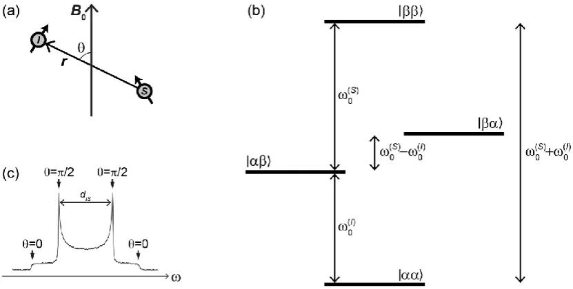
Figure 2.1. Energy levels for a single spin-½ nucleus, with and without an applied

magnetic field, . States and (with magnetic quantum numbers ±½) have energies that differ by an amount equivalent to the Larmor frequency (in rad s-1_{), which is}

— 9 —

(2.4)

Without a magnetic field, these energy levels are degenerate. In general, upon application of a magnetic field to a nucleus with spin , a total of energy levels are formed, each separated by an energy equivalent to . This is called Zeeman splitting (Figure 2.1). At equilibrium, the populations of the energy levels are determined by the Boltzmann distribution, with the result that a population difference (and hence a net magnetisation) is induced that scales with . Transitions between energy levels of a system may be stimulated by applying radio frequency (r.f.) irradiation (see section 2.2.1).

2.1.2 The Density Operator

Quantum mechanically, the physical state of a system can be represented in the bra-ket notation by a state vector, , a linear superposition of and states, i.e.

.ii _{A convenient approach for describing the state of an ensemble of spins}

is to define a density operator, :

(2.5)

where the overscore indicates an ensemble average. In matrix form, the density matrix has elements , which, for a single spin-½ nucleus is

(2.6)

With increasing numbers of spins, , the size of this matrix scales as . The diagonal elements correspond to populations of eigenstates, while the off-diagonal elements represent coherences between the eigenstates. Non-zero off-diagonal elements indicate that the phases of the involved states evolve not randomly, but to some extent in a coherent manner on average. At equilibrium in a static magnetic field, only the diagonal elements of the density matrix are non-zero. The order of coherence between two states, 1 and 2, is defined as , with the total magnetic quantum number of each state. In an NMR experiment, r.f. radiation is applied to the spin system with the aim of generating and manipulating coherences between states.

— 10 —

For any observable , it can be shown96 _{that the expectation value of its}

corresponding operator, , is simply

(2.7)

with information about the sample and relating to the measurement being contained within and respectively. is as a function of time, as the spin system evolves under the influence of the Hamiltonian, and it is this behaviour that we observe in an NMR experiment. The evolution of pure quantum mechanical states is described by the time-dependent Schrodinger equation. Derived96 _{from this is the Liouville von-Neumann}

equation, which describes how the density operator evolves in time:

(2.8)

The solution to this equation is

_(2.9) where is the total Hamiltonian, a sum of contributions that each arise from different interactions of spins with their environment. To fully understand the result of an NMR experiment, we must therefore consider these different contributions. Indeed, the true power of NMR spectroscopy lies in its ability to probe, and derive useful information from, the unique multitude of interactions present in a given sample.

2.1.3 Interaction Hamiltonians

When placed in a magnetic field, the total Hamiltonian that acts on a system of spins is

(2.10)

— 11 —

molecule. Respectively, , , , , and are Hamiltonians for the chemical shielding, the dipolar interaction, J-coupling, the quadrupolar interaction, the paramagnetic interaction and the Knight shift, and the details of each of which will be discussed below.

The Hamiltonian for each internal interaction can be written as a Cartesian tensor:

(2.11)

where is a second rank tensor representing the interaction (with elements dependent on the coordinate frame). is the spin operator for one spin, while is either the spin operator for a second spin or the external field, depending on the interaction.

In order to consider each of the interactions, it is most straightforward to deal with them in their principal axis system (PAS), a coordinate frame in which the interaction tensor is diagonal:

(2.12) However, since NMR measurements are conducted in the laboratory frame (in which the dominant Zeeman interaction lies, by convention, in the z-direction), it is necessary to rotate each interaction tensor to this frame from its individual PAS. In order that we can more easily accomplish this, we can express the interaction Hamiltonians in spherical, rather than Cartesian, tensor form:

(2.13)

The Hamiltonian is hence expressed as a sum of a number of terms with different rank and order (which can take 2 +1 values). Each term in this expansion is made up of an irreducible spherical tensor component (i.e. spatial component), , which represents

— 12 —

diagonal elements of the Cartesian tensors are non-zero, the above expression reduces to only four terms (all others are zero):

(2.14) The first of these terms is isotropic (rank 0, i.e. a scalar), while the next three terms are anisotropic (rank 2 tensors). Of these, only select terms will be non-zero depending on the interaction type, leading to further possible simplifications (see below for specific interactions). The spin operators and irreducible tensor components for the chemical shift and dipolar interactions are given in Appendix A.

The PASs for each interaction (and for each spin within a sample) are not coincident, and as such rotation of the interaction tensors in three dimensions to the laboratory frame must be through a general set of “Euler angles”, ( , , ). By common convention (and it should be noted that more than one convention is used in the literature89_{), rotation is firstly applied about the z-axis by an angle , which shifts the x-}

and y-axes. A second rotation is then applied about the “new” y-axis by an angle , shifting the x- and z-axes. This is followed finally by a rotation about the new z-axis by an angle . This set of rotations is illustrated in Figure 2.2 and can be written

(2.15)

A spherical tensor component, , is converted by rotation into a sum of components with the same rank, (i.e. a scalar will remain a scalar, while a second rank tensor will remain as such) but different order, . For a rotation from the PAS to the laboratory frame, this is given by

(2.16)

where is the rotation matrix, defined as

— 13 —

and , and are the Euler angles describing the relative orientation between the

two frames. are elements of what are known as the reduced Wigner rotation matrices, which can be found in Appendix A.

As mentioned, the interactions discussed here are much smaller than Zeeman interaction and as such can be considered as first order perturbations to the Zeeman Hamiltonian. As a consequence of this, an approximation can be made whereby in rotating to the laboratory frame only spin terms that commute with the Zeeman interaction, , are retained. This is known as the secular, or high-field, approximation. The commutator is , which is only equal to zero when =0. Therefore, in the laboratory frame,

(2.18)

Only a single isotropic component and a single anisotropic component remain. The magnitude of an anisotropic interaction depends on its orientation with respect to the magnetic field, while isotropic interactions are orientation-independent. In the solution state, the overall tumbling of molecules ensures that the nuclei within them experience effectively all possible orientations over a short time scale (e.g. ns, depending on the size

Figure 2.2. Illustration of the rotation between frames using Euler angles. The set of

— 14 —

of the molecule), and so an average of each interaction is observed. Anisotropic interactions are said to be “averaged”, and only the effects of isotropic chemical shift and J-coupling are observed.

2.1.4 Chemical Shielding

Perhaps the most valuable interaction for the majority of NMR experiments carried out is chemical shielding. Within a molecule, an applied static magnetic field ( ) induces currents in electron orbitals, generating an opposing field. The total effective field at the site of the nucleus is therefore modified:

(2.19) where is the chemical shielding tensor. Because the electron density surrounding a nucleus varies depending on the local environment of that site (e.g. its location within a molecule), the strength of the chemical shielding interaction is different for each unique nuclear environment in a molecule, leading to measurable differences in the Larmor frequencies of those nuclei. This effect is called chemical shift, and the ability to measure it and hence differentiate between nuclei that are of the same species but located in different chemical environments is one of the most powerful tools in experimental NMR.

In Cartesian form the Hamiltonian for the chemical shift interaction is

(2.20) Because the electron density is three-dimensional and in general not isotropic, is a second rank tensor. In general, the chemical shift has both an isotropic and anisotropic contributions (see Appendix A). In the PAS, is diagonal, with the terms , and

known as the principal components (where superscript denotes PAS). The isotropic chemical shift, which is invariant under rotations, can be written as the mean of these components:

— 15 —

To describe the anisotropy of the chemical shift tensor, rather than quoting the three principal components it is common to parameterise the tensor with, in addition to

, the so-called anisotropy ( ) and asymmetry ( ). These are defined asiii

(2.22)

(2.23)

In liquids, averaging by isotropic molecular tumbling averages the anisotropic component of chemical shift, so only the isotropic interaction is observed. In this case, each resonance is observed at a different location on the spectrum depending on the isotropic chemical shift (often shortened to simply the “chemical shift”), itself dependent on the local nuclear environment. Because the chemical shift interaction strength is directly proportional to the external magnetic field, in order to directly compare chemical shifts across different fields they are usually quoted with respect to the Larmor frequency of a reference compound:

(2.24) where we have used equations 2.3 and 2.19 to convert between Larmor frequencies and shielding tensors, and is in units of parts per million (ppm) owing to the relatively small magnitude of the shift when compared to the Zeeman interaction (the difference in Larmor frequencies that is due to the chemical shift is small compared to the overall Larmor frequencies). Because is now field-independent, it reflects purely the local electronic environment of the nucleus. For 1_{H and} 13_{C (and} 29_{Si), the standard reference}

compound for most applications is tetramethylsilane (TMS), although 4,4-dimethyl-4-silapentane-1-sulfonic acid (DSS) is often used for proteins as it is soluble in water and may therefore be packed along with a hydrated sample.97,98

In static solids, the lack of molecular tumbling means that the interaction is not averaged, and for different orientations the interaction strength (and hence chemical shift observed) is different. At a given angle defined by (polar and azimuthal angles

iii

— 16 —

between the chemical shielding PAS and the laboratory frame – see Ref. 89), the first order interaction strength is given by:89

(2.25) In a static powdered sample, effectively all the possible orientations are present and sum to give rise to a distinctive “powder pattern”.

2.1.5 Dipolar Coupling

As described earlier, nuclei with non-zero spin possess a magnetic moment. In a multi-spin system, these will interact with one another through space. The strength of this interaction, which is known as the direct dipole-dipole interaction (or dipolar coupling), depends on the gyromagnetic ratios of the two nuclei, the distance between them and the orientation of the dipolar vector with respect to the magnetic field (see Figure 2.3a). For coupled spins I and S,

(2.26)

where and are, respectively, the unit vector and the magnitude of the vector between the two spins, and the dipolar coupling constant:

(2.27)

in units of rad·s-1 _{Note that the inverse-cubed dependence of the interaction on the}

separation means that measurements of dipolar couplings can provide distance measurements between pairs of nuclei, which can ultimately lead to methods for determining molecular structures. Note also that the dipolar coupling is, unlike the chemical shift, independent of the field. For neighbouring nuclei within a molecule, dipolar couplings usually lie in the range of kHz to tens of kHz (e.g. a 13_C-1_{H coupling at a}

— 17 —

Figure 2.3. (a) Representation of the dipolar interaction between two nuclei ( and ),

where the interaction strength is dependent on the angle, , subtended by the internuclear vector, , and the magnetic field vector, . (b) Energy levels for two dipolar-coupled spin-½ nuclei, and , with corresponding Larmor frequencies and . (c) Pake doublet line shape of a static powdered sample that is due to the

) dependence of dipolar coupling. For each distinct value of , the line is split into a doublet with separation . When the ) dependence is integrated over a sphere, the line shape is a superposition of two mirror-image powder patterns corresponding to each of the doublet resonances. Features arising from different values of are marked. The separation between the two maxima is (or for a homonuclear coupling99_{), the dipolar coupling constant as defined in the main text of}

§2.1.5.

In Cartesian tensor form, the dipolar coupling Hamiltonian is

(2.28)

In spherical tensor notation, in the PAS, this is

(2.29)

where the rank 0 term (see equation 2.14) is zero because the dipolar tensor, , is traceless ( ) and the terms with rank 2, order ±2 are zero because is axially symmetric ( ).

Rotating into the laboratory frame gives (ignoring the terms for which

by using the secular approximationiv₎

iv _{The full expressions for}

— 18 —

(2.30) where we have substituted and looked up the relevant reduced Wigner rotation matrix element.

The spin term is given by (see Appendix A)

(2.31)

where . For the heteronuclear case (where the two coupled nuclei are of different species), the term is absent and the dipolar Hamiltonian constitutes a first order shift to the Zeeman interaction (the eigenfunctions of the operator are simply the Zeeman states, etc.). For the homonuclear case, the presence of this latter term has some interesting effects. In particular, the degenerate spin states (e.g. and states in a two-spin system) are “mixed”, so that the eigenfunctions of the spin system are linear combinations of degenerate Zeeman levels. This leads to a range of transition frequencies, resulting in Gaussian broadening of the observed lineshape.89 _{In addition, it leads to a phenomenon whereby the Hamiltonian}

does not necessarily commute with itself at different time points (the “observed” spin state of each spin varies between and ), a consequence of which is that magic angle spinning (see below) proves less efficient than in the heteronuclear case.

In the heteronuclear case, there is no degeneracy and hence only two transitions are possible. For a static powdered sample, integrating the dependence of each of these transitions over all orientations results in a so-called Pake doublet lineshape (Figure 2.3c).21

2.1.6 J-Coupling

— 19 —

(2.32)

where is the J-coupling tensor. is not traceless and as such has an isotropic (scalar) component, but while anisotropic J-coupling terms can exist100 _{they are almost always}

ignored owing to their small magnitude. The J-coupling tensor is therefore normally

written as .

The isotropic J-coupling interaction is field-independent and causes splitting of resonances in the NMR spectrum, with the components separated by an energy, given by

J (in units of Hz), of usually only a few Hz to hundreds of Hz (e.g. ~120-130 Hz for a

13_C-1_{H one-bond J-coupling). This splitting is readily observed in solution NMR}

(molecular tumbling does not average the isotropic interaction) and is a valuable tool in determining the structures of soluble molecules101_{, but such a small coupling strength}

often renders it unobservable by solid state NMR, where other interactions dominate and mask its effect. Nevertheless, in many biological samples in the solid-state, line widths (e.g. of 13_{C resonances) are narrow enough under favourable conditions for J-couplings to}

be observed.

2.1.7 Other Interactions

Nuclear species with spin >½ possess, in addition to a magnetic dipole moment, an electric quadrupole moment due to a non-spherical charge distribution at the nucleus. The interaction of this moment with electric field gradients across the nucleus is known as the quadrupolar interaction. This effect can often lead to extremely broad resonances of several MHz. For biological samples, the nuclei of interest (e.g.1_H,13_C, 15_{N) are mostly}

spin-½ only and therefore do not exhibit quadrupolar couplings. Deuterium (2_{H, spin-1)}

is used reasonably often in biological solid-state NMR (e.g. in observation of the narrowing of the lineshape by dynamics102 _{but for the purposes of this work is only used}

in the context of dilution of proton dipolar networks, and as such the details of the quadrupolar interaction will not be discussed further.

— 20 —

paramagnetic shifts.103-105 _{In addition, relaxation enhancements can be used as a tool to}

reduce the recycle time of an experiment (see §2.2.4).

Finally, the Knight shift interaction arises in metals when shielding from conduction electrons leads to an additional effective field at the nucleus. As the Knight shift only occurs in metals, it is not relevant to any of the results in this thesis.

2.1.8 Magic Angle Spinning

As has been described, many of the interactions discussed above are anisotropic in nature, meaning that their strength depends on their orientation with respect to the external magnetic field. In solution, the overall tumbling of molecules ensures anisotropic interactions are averaged. In the solid state, however, this natural averaging does not occur, and so anisotropic interactions remain directly observable. In a solid sample, where typically many (or indeed effectively all) orientations are present, NMR lines are broadened as a result of summing the resonances from each of the individual orientations. This broadening is often undesirable, as although many potentially valuable sources of information are encoded within it, excessive broadening can easily lead to poor spectral resolution and hence difficulties in extracting that information.

A common and often indispensable technique to counteract this broadening in solid-state NMR is magic angle spinning (MAS), in which samples are placed inside a “rotor” that is mechanically rotated rapidly about an axis that is oriented at the so-called “magic angle” ( =54.7°) with respect to the external magnetic field (see Figure 2.4). This method effectively attempts to emulate the molecular tumbling that occurs in liquids.

— 21 —

(2.33)

recalling that, owing to the secular approximation, is the only relevant non-scalar term in the laboratory frame. The Wigner rotation matrix for the rotation from the rotor frame to the laboratory frame is

(2.34) For one rotation of the rotor over a time ,

(2.35)

Therefore, for , and hence average to zero over one complete rotor period.

For the case,

(2.36) where the reduced Wigner rotation matrix . By setting the rotor axis, , to 54.7°, this term and hence are zero.

MAS experiments therefore aim to reduce the anisotropic components of interactions by employing sample rotation about an axis that lies at this angle with

Figure 2.4. Magic angle spinning. The sample is packed into a rotor that is mechanically

— 22 —

respect to the magnetic field. In simple terms, all components of anisotropic interactions that are parallel with the rotor axis are zero at 54.7°, while all those perpendicular are averaged to zero over a full rotor period. The faster the spinning frequency, the better this averaging. As a rule of thumb, the sample must be spun at a frequency much greater than the interaction strength (in Hz) for fully effective averaging of the interaction (for homogeneous interactions, for reasons discussed in §2.1.5, the requirements are even greater). At lower spinning frequencies, where averaging is not complete, the

terms of equation 2.33 must be considered. Full calculation involving the Wigner rotation matrices for (and taking =54.7°) yields

(2.37) This expression contains terms oscillating at frequencies of and , which give rise to so-called “spinning side bands”. The lineshape arising from an anisotropic interaction is split into a number of resonances, separated, in Hz, by integer multiples of the spinning frequency. These sidebands decrease in intensity as the spinning frequency is increased, eventually leaving only a single resonance at the isotropic chemical shift, which remains observable (as do J-couplings, which are also scalar) as in liquid-state NMR. Modern MAS technology can routinely spin samples up to frequencies of tens of kHz. Many of the experiments in this piece of work rely of state-of-the-art probes that enable spinning frequencies of up to 67 kHz (1.3 mm diameter rotors) or even 100 kHz (0.8 mm rotors). Such fast spinning can cause a large amount of frictional heating of the rotor and hence sample, an important consideration when dealing with biological samples. Additionally, the necessarily small diameters of rotors used can limit the volume of sample that can be studied, impacting negatively on experimental sensitivity.

2.2 The Pulsed-FT NMR Experiment

The NMR experiment allows an experimental scientist to probe a sample, at the molecular level, by observing the behaviour of spins over time and hence obtaining information about the various interaction Hamiltonians active in the system. In order to accomplish this, the experimentalist must perturb the system. This is achieved through the application of r.f. radiation. The total Hamiltonian becomes

— 23 —

where is the Hamiltonian representing all internal interactions (see Equation 2.10) and is the Hamiltonian for the r.f. irradiation.

Before exploring the various details of the NMR experiment, it is useful at this stage to outline its basic form. The first NMR experiments involved the simultaneous application of r.f. irradiation and a “sweeping” of the field strength through the resonance condition. Modern experiments, however, are almost exclusively performed in a pulsed manner, whereby the field is held static and r.f. irradiation is applied in short pulses. This fact, combined with the Fourier transform that is applied to the final signal, gives the technique its name – pulsed-Fourier transform (pulsed-FT) NMR.

In the simplest terms, the basic pulsed-FT NMR experiment (in its most common form) can be broken down as follows. The sample is placed into a large (e.g.

several Tesla) static magnetic field, , by packing it into an NMR tube (liquid-state) or rotor (solid-state MAS), loading this into a probe, then inserting this probe into the bore of a superconducting electromagnet. Through interacting with the nuclear magnetic moments within the sample, the magnetic field generates a net magnetisation ( ) along the axis of the field (taken to be z) that is proportional to the population difference (between aligned and anti-aligned states) induced. Each of the individual magnetic moment vectors in the sample precesses about the field axis at a frequency , but because of an isotropic distribution of phases the bulk magnetisation is stationary. Without further intervention, however, the magnetisation of the nuclei is dwarfed by, and cannot be isolated from, the diamagnetism of paired electrons.

In a “one-pulse” experiment, the spectrometer generates an r.f. signal ( , orders of magnitude weaker than ) that is applied in the form of electromagnetic radiation along an axis perpendicular to , with the effect that each of the individual nuclear magnetic moment vectors, and hence the bulk magnetisation, rotates about the axis of the pulse. The irradiation can be turned off when the bulk nuclear magnetisation lies in the x-y plane. The spins and hence bulk magnetisation continue to precess about the z-axis, an effect that is measurable through electromagnetic induction in a coil wrapped around the sample (the same coil administers the r.f. irradiation). The resulting signal, now isolated from the effect of electron pairs, is returned to the spectrometer for processing.