University of Warwick institutional repository: http://go.warwick.ac.uk/wrap
This paper is made available online in accordance with
publisher policies. Please scroll down to view the document
itself. Please refer to the repository record for this item and our
policy information available from the repository home page for
further information.
To see the final version of this paper please visit the publisher’s website.
Access to the published version may require a subscription.
Author(s): Wouter J.T. Bos, Colm Connaughton, Fabien Godeferd
Article Title: Developing homogeneous isotropic turbulence
Year of publication: 2012
Link to published article:
http;//dx.doi.org/10.1016/j.physd.2011.02.005
Publisher statement: “NOTICE: this is the author’s version of a work
that was accepted for publication in Physica D: Nonlinear Phenomena.
Changes resulting from the publishing process, such as peer review,
editing, corrections, structural formatting, and other quality control
mechanisms may not be reflected in this document. Changes may
have been made to this work since it was submitted for publication. A
definitive version was subsequently published in Physica D: Nonlinear
Phenomena, [VOL:241, ISSUE:3,Febriary2012] DOI:
arXiv:1006.0798v2 [nlin.CD] 6 Nov 2010
Wouter J.T. Bos,1,∗ Colm Connaughton,2,† and Fabien Godeferd1,‡
1
Laboratoire de M´ecanique des Fluides et d’Acoustique,
CNRS UMR 5509, ´Ecole Centrale de Lyon, France, Universit´e de Lyon
2
Mathematics Institute and Centre for Complexity Science, University of Warwick, Coventry CV4 7AL, UK
We investigate the self-similar evolution of the transient energy spectrum which precedes the establishment of the Kolmogorov spectrum in homogeneous isotropic turbulence in three dimensions using the EDQNM closure model. The transient evolution exhibits self-similarity of the second kind and has a non-trivial dynamical scaling exponent which results in the transient spectrum having
a scaling which is steeper than the Kolmogorov k−5/3
spectrum. Attempts to detect a similar phenomenon in DNS data are inconclusive owing to the limited range of scales available.
PACS numbers: 47.27.Gs,47.27.eb
INTRODUCTION TO TRANSIENT SPECTRA IN TURBULENCE
Although a large amount of work has been done char-acterising the properties of the Kolmogorovk−5/3
spec-trum of three dimensional turbulence, rather less atten-tion has been paid to the transient evoluatten-tion which leads to its establishment. This transient evolution is essen-tially non-dissipative since it describes the cascade pro-cess before it reaches the dissipation scale. Part of the reason why this process has attracted relatively little at-tention is that this transient evolution is very fast, typ-ically taking place within a single large eddy turnover time. It is thus of little relevance to the developed tur-bulence regime of interest in many applications. Never-theless, one may ask whether this developing turbulence, as one might call this transient regime, displays any in-teresting scaling properties. Previous studies of the de-veloping regime in weak magnetohydrodynamic (MHD) turbulence [1] suggest that this transient regime might have non-trivial scaling properties: in this case it was found that the establishment of the Kolmogorov spec-trum is preceded by a transient specspec-trum which is steeper than the Kolmogorov spectrum. This latter is, in turn, set up from right to left in wavenumber space only after the transient spectrum has reached the end of the inertial range and started to produce dissipation.
Subsequent studies suggest that this behaviour, in par-ticular the occurence of a non-trivial dynamical scaling exponent, is typical for turbulent cascades which are fi-nite capacity - meaning that the stationary spectrum can only contain a finite amount of energy. The Kolmogorov spectrum of three dimensional turbulence is in the class of finite capacity systems, as we shall see below. There are, however, examples of other turbulent cascades which are not - infinite capacity cascades are common in wave turbulence for example [2]. In addition to the MHD cas-cade mentioned above, examples of non-trivial scaling exponents in finite capacity cascades have been found in developing wave turbulence [3, 4], Bose-Einstein
conden-sation [5, 6] and cluster-cluster aggregation [7]. Although a possible heuristic explanation of the transient scaling in the MHD context has been put forward in [8], this heuris-tic relies heavily on the anisotropy of the MHD cascade and does not seem readily generalisable to other contexts. In general, the transient exponent is associated with a self-similarity problem of the second kind [9]. From a mathematical point of view, its solution requires solving a nonlinear equation in which the exponent appears as a parameter which is fixed by requiring consistency with boundary conditions. It is probably unrealistic to expect that there is a general heuristic argument capable of re-solving such a mathematically challenging problem. This is not to say, however, that particular cases may not be amenable to heuristic arguments which take into account the underlyingphysicalmechanisms driving the transient evolution rather than taking a purely mathematical point of view.
This issue has not yet been studied in the context of homogeneous isotropic turbulence. Investigations of transient spectra in the classical Leith closure model [10] have suggested, however, that the transient spec-trum of developing homogeneous isotropic turbulence is indeed non-trivially steeper than k−5/3 [11]. In this
work, we investigate the transient evolution of homo-geneous isotropic turbulence using the Eddy-Damped Quasi-Normal Markovian (EDQNM) closure model and direct numerical simulation (DNS) of the Navier-Stokes equation.
The transient spectrum might be expected to evolve self-similarly. In other words there is a typical
wavenum-ber, s(t), which grows in time, and a dynamical scaling
exponent,a, such that
Ek(t)≍c s(t)aF(ξ) whereξ=s(t)k . (1)
Here≍denotes the scaling limit: k→ ∞,s(t)→ ∞with ξ fixed and c is an order unity constant which ensures thatEk(t) has the correct physical dimensions, L3T−2.
2
finite time corresponding to a cascade which accelerates “explosively”. The direct cascade in 3D turbulence is of this type. The characteristic wavenumber is most easily defined as a ratio of moments of the energy spectrum. Let us define
Mn(t) = Z ∞
0
knEk(t)dk. (2)
Eq. (1) suggests that the ratio Mn+1(t)/Mn(t) is
pro-portional to s(t) so that we may define a typical scale intrinsically by
sn(t) =Mn+1(t)
Mn(t) . (3)
A little caution is required: we must takensufficiently high to ensure that the moments Mn(t) used in
defin-ing the typical scale, converge at zero. Otherwise, the integral is dominated by the initial condition or forcing scale and does not capture the scaling behaviour. In this paper, we mostly taken= 2, which turns out to be suf-ficient for our purposes, although we will compare the behaviour obtained for n = 2 andn= 3 in our numer-ical simulations to assure the reader that the picture is consistent.
We would like to emphasise that the self-similar tran-sient dynamics which we study in this paper occurbefore
the onset of dissipation. This is in contrast to the tran-sient dynamics describing the long time decay of homoge-neous isotropic turbulence after the onset of dissipation which are also believed to exhibit self-similarity. See [12] for recent experiments and a review of previous work. Some numerical results on the long time transient dy-namics of the EDQNM model can be found in [13]. The pre-dissipation transient occurs very quickly. Indeed, as we shall see, the typical scale, s(t), in this regime di-verges as s(t)∼(t∗
−t)b where t∗ is the time at which
the onset of dissipation occurs (typically less than a sin-gle turnover time) and b <0. For finite Reynolds num-ber, this singularity is regularised by the finiteness of the dissipation scale. The fact that, in the limit of infinite Reynolds number, the typical scale can grow by an arbi-trary amount in an arbitrarily small time interval ast∗
is approached explains the statement often found in the literature that the Kolmogorov spectrum is established quasi-instantaneously in the limit of large Reynolds num-ber.
THE EDQNM MODEL
In this section we examine the self-similar solutions of the EDQNM model [14]. The structure of the EDQNM model can be obtained in different ways. One way is starting from the Quasi-Normal assumption [15]. An-other way is by simplifying the Direct Interaction Ap-proximation [16] which was obtained by applying a renor-malized perturbation procedure to the Navier-Stokes
equation. It is thus directly related to the Navier-Stokes equation, unlike the Leith model which was heuristically proposed to capture some features of the nonlinear trans-fer in isotropic turbulence. However, recent work [17] showed that the structure of the Leith model can be ob-tained by retaining a subset of triad interactions involv-ing elongated triads from closures like EDQNM. Since EDQNM contains a wider variety of triad interactions, it is able to capture more details of the actual dynamics of Navier-Stokes turbulence, as for example illustrated in [18]. At the same time it has the advantage over DNS that much higher Reynolds numbers can be obtained.
The EDQNM model closes the Lin-equation by ex-pressing the nonlinear triple correlations as a function of the energy spectrum,
∂Ek
∂t = T [Ek]−2ν k
2E
k (4)
whereν is the viscosity and T [Ek] represents the
nonlin-ear interactions between different scales. T [Ek] has the
form
T [Ek] = Z
∆
dk1dk2Tk,k1,k2k(k1k2)
−1E k2(k
2E k1−k
2 1Ek),
(5) where ∆ signifies that the region of integration is over all values ofk1andk2 for which the triad (k, k1, k2) can
form the sides of a triangle and the interaction strength of each triad,Tk,k1,k2, is given by
Tk,k1,k2=
k1
k(θkθk1+θ
3 k2)
1−exp [−(µk+µk1+µk2)t]
µk+µk1+µk2
.
(6) whereθ,θ1 andθ2are the cosines of the angles opposite
tok,k1andk2respectively in the triangle formed by the
triad (k, k1, k2) and
µk=ν k2+λ
s Z k
0
p2E
pdp, (7)
is the timescale associated with an eddy at wavenumber
k, parameterised by the EDQNM parameter,λ, which is
chosen equal to 0.49, [19]. For a full discussion of the origins and properties of the EDQNM model see [20, 21]. We concern ourselves here only with the inviscid limit whereν→0.
If we substitute the scaling ansatz, Eq. (1) into Eq. (4) withν= 0 then, in the scaling limit, the nonlinear trans-fer term becomes homogeneous of degree 3+32a in sand one finds
ds
dt =
√
c s5+2a (8)
a F −ξdF
dξ = T [F]. (9)
Scaling alone does not determine the dynamical exponent
a. To determine awe may attempt to impose
constraint which will fix a. Let us go down this path, at first naively, and then reconsider our argument more carefully:
1.Forced case
If we consider forced turbulence, then energy is injected into the system in a narrow band of low wavenumbers (which necessarily lie outside of the region of applicability of the scaling solution). The total energy grows linearly in time (remember we are interested in the dynamics before the onset of dissipation): R∞
0 Ek(t)dk=ǫ t. If we use the
scal-ing ansatz, Eq. (1), differentiate with respect to time and rearrange we obtain
ds
dt =ǫ
(a+ 1)c
Z ∞
0
F(ξ)dξ
−1
s−a. (10)
Taken together with Eq. (8) we are led to expect
a=−53 for forced turbulence. (11)
The same conclusion would be reached by dimen-sional analysis of Eq. (1) under the assumption that the sole parameter available is the energy flux, ǫ, (having physical dimension L2T−3).
2.Unforced case
In unforced turbulence, the energy is supplied solely through the initial condition which is taken to be supported in a narrow band of low wavenum-bers (which, again, lie outside of the region of ap-plicability of the scaling solution). In extremis, one could take Ek(0) = E0δ(k). In the time
window of interest (before the onset of dissipa-tion), the total energy remains constant in time:
R∞
0 Ek(t)dk=E0. In this case, the scaling ansatz,
Eq. (1), immediately yields:
a=−1 for unforced turbulence. (12)
The same conclusion would be reached by dimen-sional analysis of Eq. (1) under the assumption that the sole parameter available is the initial energy,E0
(having physical dimension L2T−2).
Note that upon subsitution into Eq. (8) both cases, Eq. (11) and Eq. (12), predict explosive growth of the characteristic wavenumber. This is in line with expecta-tions: it is widely believed that onset of dissipation in the direct cascade is set by the large scale eddy turnover time rather than the Reynolds number. This explosive growth is the key to understanding why these arguments for the value of the exponentaare flawed. In both cases we assumed implicitly that the integral,R∞
0 F(ξ)dξdoes
not diverge at its lower limit (it does not diverge at its
upper limit sinceF(ξ) decays exponentially for large val-ues ofξ). In order to study this issue, let us assume that F(ξ) has power law asymptotics near 0:
F(ξ)∼A ξ−x as ξ
→0. (13)
The exponent x is the spectral exponent of the tran-sient spectrum. In the case that s(t) diverges in finite time, then this assumption of power law asymptotics for F(ξ) taken together with the scaling ansatz requires that
x=−a. To choose otherwise would result in the large
scale part of the energy spectrum either diverging or van-ishing at the onset of dissipation, neither of which is ac-ceptable. Both values of a = −5/3 and a = −1 thus result in divergence of R∞
0 F(ξ)dξ rendering our
argu-ments inconsistent. In the latter (unforced) case, this di-vergence is only logarithmic allowing us, perhaps, to hope that it does not ruin the scaling argument completely. We shall see from numerical measurements however, that the unforced case looks much more like the forced case (see Figs.1 and 2) from the point of view of the scaling part of the spectrum and the exponenta=−1 seems to play no role.
We have arrived at a conclusion which is unsurpris-ing given the previous work on the analogous problem in wave turbulence: the problem of the transient evolu-tion of the Kolmogorov spectrum exhibits self-similarity of thesecondkind [9] so the dynamical scaling exponent, a, cannot therefore be determined from dimensional con-siderations and we must either try to solve Eq. (9) as a nonlinear eigenvalue problem and hope that it deter-mines aor return to trying to solve the original kinetic equation. We do the latter, necessarily numerically.
NUMERICAL MEASUREMENTS OF TRANSIENT SPECTRA
We performed simulations of the EDQNM model in the unforced case by integrating numerically Eq. (4), starting from an initial spectrum,
Ek(0) =Bk4exp−(k/kL)2, (14)
with B chosen to normalize the energy to unity and kL = 0.01. The initial Taylor-scale-Reynolds number is
of order 109and the resolution is chosen 24 gridpoints per
decade, logarithmically spaced. A sequence of snapshots ofEk(t) before the viscous dissipation became
apprecia-ble are shown in Fig. 1. To find the value of the dynam-ical exponent we should find the value ofa which gives the best data collapse under the scaling ansatz, Eq. (1). We defined the typical wavenumber,s(t), to be the ra-tio,M3(t)/M2(t) of the third to the second moments of
4 10-12 10-10 10-8 10-6 10-4 10-2 100 102
10-3 10-2 10-1 100 101 102 103 104
E(k,t) k s(t)=0.02 s(t)=0.10 s(t)=1.00 s(t)=10.2 s(t)=91.4 s(t)=842 10-6 10-2 102 106
10-4 10-2 100 102
F(
ξ
)
ξ
Data rescaled by Eq.(1)
[image:5.612.357.533.58.226.2]x-1.88
FIG. 1: Time evolution of the energy spectrum, E(k, t), of
the EDQNM model in the decay case. The main panel shows
snapshots ofE(k, t) at a succession of times. The inset shows
the data collapsed according to Eq. (1) with a = 1.88 and
s(t) =M3(t)/M2(t).
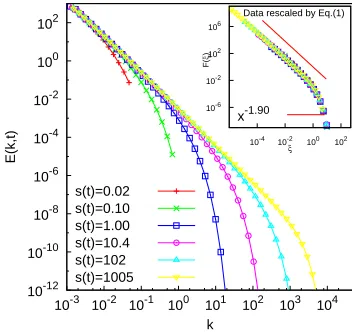
10-12 10-10 10-8 10-6 10-4 10-2 100 102
10-3 10-2 10-1 100 101 102 103 104
E(k,t) k s(t)=0.02 s(t)=0.10 s(t)=1.00 s(t)=10.4 s(t)=102 s(t)=1005 10-6 10-2 102 106
10-4 10-2 100 102
F(
ξ
)
ξ
Data rescaled by Eq.(1)
x-1.90
FIG. 2: Time evolution of the energy spectrum, E(k, t), of
the EDQNM model in the forced case. The main panel shows
snapshots ofE(k, t) at a succession of times. The inset shows
the data collapsed according to Eq. (1) with a = 1.90 and
s(t) =M3(t)/M2(t).
decade of scales to forget the initial condition (which had s(0)≈0.02). This procedure gave 1.88±0.04 where the error estimate is the standard deviation of the distribu-tion of minima obtained by bootstrapping the minimiza-tion procedure on randomly selected subsets of the total set of snapshots obtained from the numerical simulation. The data collapse thus obtained, shown in the inset of Fig. 1, is of high quality thereby supporting the scaling ansatz. 10-3 10-2 10-1 100 101 102 103 104
0 500 1000 1500 2000 2500 3000 3500 sn
(t) = M
n+1
(t) / M
n (t) t n=2 n=3 1 1.5 2 2.5
0.001 0.1 10 1000 s3
(t)/s
2
(t)
[image:5.612.89.267.63.230.2]s2(t) Scaling with higher moments
FIG. 3: Time evolution of the typical scale,sn(t), as defined
by Eq.(3), of the EDQNM model in the forced case for
dif-ferent choices ofn. The main panel demonstrates thats2(t)
ands3(t) show the same qualitative behaviour with a finite
time singularity which is regularised by the onset of
dissipa-tion. The inset illustrates that the ratios3(t)/s2(t) is
approx-imately constant as the typical scale (as measured bys2(t))
grows over several decades.
Corresponding results for the case of forced turbulence are presented in Fig. 2. The simulation was forced by keeping the energy in the first two wavenumber shells fixed in time. Performing the same analysis on the data as for the unforced case, the optimal data collapse (shown in the inset of Fig. 2) occurs for a value of the dynamical scaling exponent of 1.90±0.05. This is consistent with the value obtained for the unforced case.
[image:5.612.89.265.342.508.2]As a final set of checks on the consistency of our nu-merical simulations with the scaling hypothesis, Eq. (1), Fig. 3 shows the evolution in time (for the forced case) of the typical scale,sn(t) as defined in Eq. (3), forn= 2
andn = 3. The fact that s(t) diverges in finite time is clearly evident from the main panel as is the fact that the qualitative behaviour is the same regardless of the choice
ofn. More quantitatively, the inset of Fig. 3 shows that
the ratio of the typical scales obtained by taking n= 3 andn= 2 is approximately constant over a large range of values ofs2(t). The typical scales obtained for
differ-ent values of nare therefore proportional to each other in the scaling regime,s(t)→ ∞(the subsequent decrease afters(t)≈100 is due to the onset of dissipation). These results justify our earlier comment that the scaling anal-ysis is insensitive to the choice of ratio of moments used to define the typical scale provided these moments are of sufficiently high order.
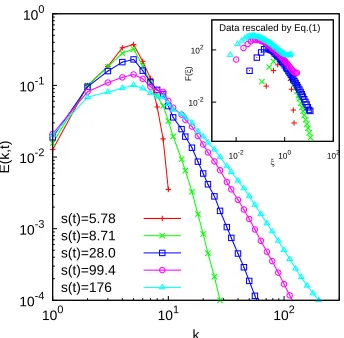
10-4 10-3 10-2 10-1 100
100 101 102
E(k,t)
k s(t)=5.78
s(t)=8.71 s(t)=28.0 s(t)=99.4 s(t)=176
10-2 102
10-2 100 102
F(
ξ
)
ξ
[image:6.612.94.266.59.228.2]Data rescaled by Eq.(1)
FIG. 4: Time evolution of the energy spectrum,E(k, t), in a
direct numerical simulation of the decay case. The main panel
shows snapshots ofE(k, t) at a succession of times. The inset
shows the data collapsed according Eq. (1) witha= 1.47 and
s(t) =M3(t)/M2(t).
the same within our estimated range of uncertainty. This is quite different from infinite capacity cascades where constraints imposed by conservation laws result in dif-ferent transient scaling exponents for the forced and un-forced cases [23]. Secondly, the measured transient ex-ponents are discernibly different from either of the naive values argued in Eq. (12) or Eq. (11). This confirms our expectation that the transient scaling is different from Kolmogorov. Thirdly, the fact thatais larger than 5/3 means that the transient spectrum is considerablysteeper
than the Kolmogorov spectrum. The latter is then set up from right to left in wavenumber space after the on-set of dissipation. This transition from the steeper spec-trum to k−5/3 also evolves quasi-instantaneously in the
same sense as the pre-dissipation transient does. It very quickly sets up the usual Kolmogorov spectrum over all scales once the onset of dissipation has occured. This spectrum then decays globally for all subsequent time as detailed, for example, in [13]. The EDQNM equation is therefore no different to any of the other finite capac-ity cascades which have been investigated to date, all of which showed this behaviour. The measured value of the dynamical exponent is remarkably close to the value of 1.86 measured for the Leith model [11]. This is consis-tent with recent arguments of Clark et al. [17] suggesting that the Leith model can be obtained from rational clo-sure models by keeping only a subset of the wavenumber triads.
Given that we expect this kind of transient behaviour to be generic, we close this study with an attempt to mea-sure the corresponding dynamical scaling in a DNS of the full Navier-Stokes equation. A classical Fourier
pseudo-spectral method is used to solve the semi-implicit form of the Navier-Stokes equations with tri-periodic boundary conditions, at a resolution of 10243 [24]. Full de-aliasing
is performed to remove spurious Fourier coefficients, time marching is done with a third-order Adams-Bashforth ex-plicit scheme, while the viscous term is solved imex-plicitly. The initial velocity conditions consist of a random gaus-sian field whose energy spectrum is of the form of (14) al-though with a peak atkL= 4.52 instead of 0.01. The
re-sults are shown in Fig. 4. Proceeding as described above, we obtaineda= 1.47±0.24. The result is therefore incon-clusive as one might expect given the very short scaling range available in DNS data (as compared to numerical solutions of the EDQNM equation).
CONCLUSION
To summarise, we have investigated the self-similar evolution of transient spectra in three dimensional turbu-lence using numerical solutions of the EDQNM equation and full DNS data. These transients develop before the onset of dissipation and lead to the establishment of the Kolmogorov spectrum. We argued that the self-similarity is of the second kind allowing the transient scaling to be anomalous in the sense that it cannot be determined from dimensional considerations. This is supported by numerical data for the EDQNM equation which gave a transient exponent of 1.88 compared to the Kolmogorov value of 5/3. Corresponding measurements for the DNS data were inconclusive owing to the relatively short scal-ing range available. Nevertheless we would expect, based on our results, that a DNS at sufficiently high Reynolds number would see a steeper transient spectrum. The most relevant message from this work for turbulence re-search is probably not the value of the transient exponent itself, since few applications care about this early stage regime. Rather it is the fact that such a non-Kolmogorov scaling exists in the first place which serves as a reminder that, while thek−5/3scaling is quite robust when the
en-ergy flux through the inertial range is constant, it is not the sole scaling law consistent with the transfer of en-ergy to small scales in turbulence when the constant flux requirement is relaxed.
∗ Electronic address: [email protected]
† Electronic address: [email protected]
‡ Electronic address: [email protected]
[1] S. Galtier, S. Nazarenko, A. Newell, and A. Pouquet, J.
Plasma Phys.63, 447 (2000).
[2] A. Newell, S. Nazarenko, and L. Biven, Physica D
152-153, 520 (2001).
[3] C. Connaughton, A. Newell, and Y. Pomeau, Physica D
6
[4] C. Connaughton and A. C. Newell, Phys. Rev. E 81,
036303 (2010).
[5] R. Lacaze, P. Lallemand, Y. Pomeau, and S. Rica,
Phys-ica D152-153, 779 (2001).
[6] C. Connaughton and Y. Pomeau, Comptes Rendus
Physique5, 91 (2004).
[7] M. Lee, J. Phys. A: Math. Gen.34, 10219 (2001).
[8] S. Galtier, A. Pouquet, and A. Mangeney, Phys. Plasmas
12, 092310 (2005).
[9] G. Barenblatt,Scaling, self-similarity, and intermediate
asymptotics(CUP, Cambridge, 1996).
[10] C. E. Leith, Phys. Fluids10, 1409 (1967).
[11] C. Connaughton and S. Nazarenko, Phys. Rev. Lett.92,
044501 (2004).
[12] P. Lavoie, L. Djenidi, and R. A. Antonia, J. Fluid Mech.
585, 395 (2007).
[13] M. Lesieur, O. M´etais, and P. Comte,Large Eddy
Simu-lations of Turbulence (CUP, Cambridge, 2005).
[14] S. Orszag, J. Fluid Mech.41, 363 (1970).
[15] A. Monin and A. Yaglom, Statistical fluid mechanics
(MIT press, Cambridge, 1975).
[16] R. Kraichnan, J. Fluid Mech.5, 497 (1959).
[17] T. Clark, R. Rubinstein, and J. Weinstock, J. Turbulence
10, 1 (2010).
[18] W. J. T. Bos and J.-P. Bertoglio, Phys. Fluids18, 071701
(2006).
[19] W. J. T. Bos and J.-P. Bertoglio, Phys. Fluids18, 031706
(2006).
[20] M. Lesieur,Turbulence in Fluids (Springer, Heidelberg,
2008).
[21] P. Sagaut and C. Cambon,Homogeneous turbulence
dy-namics (CUP, Cambridge, 2008).
[22] S. Bhattacharjee and F. Seno, J. Phys. A–Math. Gen.
34, 6375 (2001).
[23] C. Connaughton and P. Krapivsky, Phys. Rev. E 81,
035303(R) (2010).
[24] F. S. Godeferd and C. Staquet, J. Fluid Mech.486, 115