Verifying The Practical Use of the Schedule Based Method

BSc Thesis

Goudappel Coffeng - University of Twente

10-12-2019

Verifying The Practical Use Of

The Schedule Based Method

Author: Karsten Hilbrands

Internal Supervisor: Dr. Konstantinos Gkiotsalitis

External Supervisor: Dr. ir. Ties Brands

P

REFACE

This thesis is the final step of my bachelor in Civil Engineering. It is the result of 13 weeks conducting my bachelor research at Goudappel Coffeng. After successfully completing this part, I will receive my Bachelor’s degree in Civil Engineering at the University of Twente in Enschede.

Goudappel Coffeng has provided me with the assignment and the resources to carry it out. Goudappel Coffeng is a consulting company in mobility. The company is active in almost all aspects of

transportation. They have approximately 200 employees divided between their five offices across The Netherlands (Goudappel Coffeng, 2019). I liked working at Goudappel and I thank the company for their resources, which made this thesis possible.

I would like to show my gratitude to the people who have made this possible for me. At the company, Ties Brands was my supervisor, he is a consultant in public transport. Ties did this together with Dennis Roelofsen. Dennis is also a consultant within the public transport department of Goudappel Coffeng. I am very thankful for their help and the good conversations we had, which pushed me in the right directions. I would also like to thank Konstantinos Gkiotsalitis, my supervisor from the

University. The useful feedback he gave, brought my thesis to a higher level.

I would like to give a special mention to Jamie Cook, who is a consultant at VLC. Jamie made changes to the algorithm in order it to make it work correctly, he also helped me in understanding the algorithm better. Further, I thank the colleagues at the ‘flex plein’, who helped me with a lot of issues in

OmniTRANS. I also want to pay my gratitude to my family, friends and roommates, for their support. In the end, I would like to thank Roos for her endless support, before and during the bachelor

S

UMMARY

To predict (passenger)loads on public transport services, models have to be used. Determination of loads, is called a route assignment. Two methods are used to perform the assignment, these are schedule based and frequency based methods. The frequency based method is a static assignment method, which makes no use of time. The schedule based method is a dynamic method, which does take time into account.

Schedule based methods provide more detailed calculations. These highly detailed calculations, require more input and are the cause of high computation times. Frequency based methods cannot make very detailed calculations. The low level of detail makes it easier to make calculations when limited data is available. Computation times of the frequency based assignment are also much smaller. In practice frequency based method are used more.

There is a lot of understanding in the improvements a schedule based approach can provide in theoretical sense. However, current literature lacks at giving a clear practical comparison between schedule and frequency based approaches. It is not known how large the improvements are and to what extend certain situations need to be modelled with schedule base methods.

This study must: give more insights in the schedule based algorithm, facilitate the use of this method and gain more knowledge about the benefits of the schedule based method compared to the

disadvantages. A recommendation in the usage of both methods should also be given. The main research question is: What are the main differences between the schedule based and frequency based methods in a practical application and what influences these differences?

A case study is used to analyse the differences between the methods and to get more understanding in the schedule based method. The study is carried out on a model of the Dutch rail network, inside the OmniTRANS software package. First, a verification of the schedule based results is carried out. This is done by comparing the in-vehicle travel time. Next, all skim results are compared. Differences between the results of both methods become clear by this method. At last, a sensitivity analysis is done with the schedule based method. This is done to see the influence of certain parameters on the run-time and the skim results. From the sensitivity analysis, a good configuration of the schedule based method can be derived.

The results of the case study show that travel times from the schedule based assignments are higher on average. Transfer waiting times came out to be lower on average for the schedule based method, which results in total lower waiting times. It can also be seen that median travel times for OD-pairs with the same characteristics are almost equal for both methods. The sensitivity analysis makes clear that the branch and bound and access waiting time settings have large influence.

There are many differences between the schedule based and frequency based methods. Many differences can be found in the application of the methods. Other route choices, caused by the

temporal aspects of the schedule based method, are the reason for larger overall travel times. Transfer time calculation seems to be done more accurately by schedule based methods. Overall, the schedule based method also gives results closer to the ‘real world’ travel times. It can be said that for some scenarios the schedule based method is a better way of assigning travellers on routes.

It is recommended to use schedule based assignments in situation were a lot of data is already

T

ABLE OF

C

ONTENTS

Preface ... II

Summary ... III

List of figures ... VI

List of tables ... VII

1. Introduction ... 1

1.1 Motivation ... 1

1.2 literature review ... 2

1.3 problem and relevance ... 4

1.4 Research Aim ... 4

1.5 Research Lay-out ... 5

2 Methodology of Assignment Methods ... 7

2.1 Public transport modelling ... 7

2.2 algorithm description ... 9

2.3 application of algorithms ... 13

3 Case Study ... 17

3.1 Dutch National Rail Model ... 17

3.2 ‘real world’ data ... 17

3.3 Skim gathering ... 18

3.4 Skim comparison ... 19

3.5 Sensitivity analysis ... 19

4 Results ... 21

4.1 Skim comparison ... 21

4.2 In-depth analysis ... 26

4.3 Sensitivity of parameters ... 28

5 Conclusions ... 31

5.1 Sub-Questions ... 31

5.2 Main Research Question... 32

6 Discussion and Recommendation ... 33

6.1 Limitations... 33

6.2 Interpretation of results... 33

6.3 Recommendation ... 34

References ... 35

Appendices ... 37

B. Settings ... 41

C. Test network results ... 42

D. Waiting time results ... 44

E. graphs sensitivity analysis ... 46

F. Amount of Connected skims ... 51

G. in-Depth Description of an Example ... 52

H. Relative Scatter Plot In-Vehicle Comparison ... 53

L

IST OF FIGURES

Figure 1: VIRM Train (rhemkes, 2019) ... I

Figure 2: Lay-Out of the Research ... 6

Figure 3: Network with one transit line and three stops (Brands, Romphc, Veitche, & Cook, 2014) .... 7

Figure 4: Four-step model (Veitch & Cook, 2013) ... 8

Figure 5: General scheme of transit assignment models (Nuzzolo, Transit Path Choice and Assignment Model Approaches, 2007) ... 8

Figure 6: A Connection Tree (Friedrich, Hofsäß, & Wekeck, 2001) ... 11

Figure 7: Effect of logit scaling parameter (Veitch & Cook, 2013) ... 13

Figure 8: Overview of the National Rail Model ... 17

Figure 9: Histogram In-Vehicle Difference ... 21

Figure 10: In-Vehicle Travel Time Difference over Demand ... 22

Figure 11: Histogram Total Travel Time Difference ... 23

Figure 12: Histogram Waiting Time Difference ... 24

Figure 13: Difference in Penalties ... 25

Figure 14: Travel Time over Distance Categories... 25

Figure 15: Travel Time over Nr. of Transfers ... 26

Figure 16: Median Travel Time Sensitivity Analysis ... 28

Figure 17: Median Travel Time Difference Sensitivity Analysis ... 28

Figure 18: Groningen - Schiphol: Transfer at Meppel ... 39

Figure 19: Groningen - Schiphol: Transfer at Assen ... 40

Figure 20: Travel time Difference in test network ... 42

Figure 21: Travel Time in Test Network over Frequency ... 42

Figure 22: Histogram Access Waiting Time Difference ... 44

Figure 23: Histogram Transfer Waiting Time Difference ... 45

Figure 24: Travel Time over Time Steps ... 46

Figure 25: Travel Time Difference over Time Step Size ... 46

Figure 26: Travel Time over Branch and Bound Settings ... 47

Figure 27: Travel Time Difference over Branch and Bound Settings ... 47

Figure 28: Travel Time over Maximum Number of Transfers ... 48

Figure 29: Travel Time Difference over Maximum Number of Transfers ... 48

Figure 30: Nr. of Connected Skims over Maximum Nr. of Transfers ... 48

Figure 31: Travel Time over Access Waiting Time ... 49

Figure 32: Travel Time Difference over Access Waiting Time ... 49

Figure 33: Nr. of Connected Skims over Maximum Access Waiting Time ... 49

Figure 34: Travel Time over Number of Skims ... 50

Figure 35: Travel Time Difference over Number of Skim Values ... 50

Figure 36: Amount of Connected Skim Values ... 51

L

IST OF TABLES

Table 1: Differences between methods ... 3

Table 2: Connection split: three connections with fixed headway (Friedrich, Hofsäß, & Wekeck, 2001) ... 13

Table 3: Connection split: adding an identical connection (Friedrich, Hofsäß, & Wekeck, 2001) ... 13

Table 4: Connection split: adding an fast connection (Friedrich, Hofsäß, & Wekeck, 2001) ... 13

Table 5: Options for a single time slot ... 15

Table 6: Options for assignment over entire hour ... 15

Table 7: Results for SB assignment... 16

Table 8: Branch and Bound Settings ... 20

Table 9: Settings sensitivity analysis ... 20

Table 10: Accuracy of Results ... 22

Table 11: Relative Difference of Travel Times ... 23

Table 12: Relative Difference of Waiting Times ... 24

Table 13: In-Depth Analysis: Average Results ... 27

Table 14: Time Step Size Run-time ... 29

Table 15: Branch and Bound Run-time ... 29

Table 16: Maximum Transfers Run-time ... 30

Table 17: Maximum Access Wait Time Run-time ... 30

Table 18: Tests for min. nr. of skims... 30

Table 19: SB Settings of application in Test Network ... 41

Table 20: FB Settings of application in Test Network ... 41

Table 21: SB settings for main skim comparison ... 41

Table 22: FB settings for main skim comparison ... 41

Table 23: Relative Difference of Access Waiting Times ... 44

Table 24: Relative Difference of Transfer Waiting Times ... 45

Table 25: Percentage of skims per OD-pair ... 51

Table 26: Results of SB Assignment on Example ... 52

Table 27: Skim Results of Example ... 52

Table 28: High Frequency In-Depth Analysis ... 54

Table 29: Low Frequency In-Depth Analysis ... 54

Table 30: Transfer Required In-Depth Analysis ... 55

Table 31: Alternating In-Depth Analysis ... 55

Table 32: Direct In-Depth Analysis ... 55

Table 33: Short Distance In-Depth Analysis ... 56

1.

I

NTRODUCTION

In this chapter the subject of this study is presented. First a motivation is given and then a literature review is done to come to a problem statement. Subsequently the research questions are formulated and a lay out of the research is given.

1.1

M

Since the start of the industrial revolution, public transport plays an important role in mobility. Recent developments, as congested roads and climate change, are causing an even larger load on public transport. These increased loads create the need for a better and higher quality public transport. The Dutch government wants to invest in more high quality services at places where they are needed most (Rijksoverheid, 2019). It is essential that the suitable services are selected prior to the investments. Selection of services can only be done by predicting loads on transit services. For these reasons, a realistic way of forecasting loads on public transport services is very important.

In the real world, public transport (PT) and everything that has to do with it, are very complex processes. Models are useful to make abstractions or idealisations of the real world. The best models use a balanced combination of fast and easy calculations and accurate results. The choice of transport mode, the travel time or the amount of passengers, can be computed with the use of certain models. Since these outputs all depend on large amounts of variables, it is hard to calculate them without a model that simplifies the real world.

Loads on transit lines are determined by predicting the routes and modes of transport that are chosen by travellers between a certain origin to destination pair (OD-pair). This helps at creating new

timetables and high quality PT networks (Guis & Nijënstein, 2015). This information can also be used to make better models for PT services. The process of forecasting the users of a route between origin and destination (O and D) is called the transit route assignment. There are two main approaches of the transit assignment: frequency based and schedule based (Liu, Bunker, & Ferreira, 2010). Predicting the usage of a transit line is based on the characteristics of that certain line. These characteristics are called the skims.

The frequency based (FB) approach can be seen as a static transit assignment. Static assignments are characterised by the lack of temporal components. The schedule based (SB) method is a within-day dynamic transit assignment which incorporates temporal aspects. In general, the FB method makes use of frequencies of transit lines and the SB approach makes use of timetable information of transit lines. FB is a more simplified method and is therefore faster to use, however, as with most simplifications, this has some limitations with respect to detailed calculations. The SB method requires more detailed input and gives more detailed results, this makes the SB method more time-consuming. (Liu, Bunker, & Ferreira, 2010)

Despite the limitations of the FB algorithm this method is still the standard for the transit network assignment. FB models are less expensive to construct and take much less computing time compared to SB methods. FB methods do not require segmentations of OD matrices or any simulation of a timetable. (Cascetta & Coppola, 2016)

1.2

In this review, the differences and (dis)advantages of the schedule based assignment according to the literature are reviewed.

The FB method has more disadvantages in theoretical sense than it has advantages in practical sense. The practical advantages for this method are primarily focussed on the run-time and costs, which are both relatively low. Within a complex PT network it is more easy and faster to use a FB approach. In general, FB approaches are useful when high levels of detail are not necessary according to (Nuzzolo, Transit Path Choice and Assignment Model Approaches, 2007). This characteristic of the FB approach is also a shortcoming. Since there are differences in amounts of passengers during the day and within hours, dynamic time components become very important. During rush hours, there are peaks of travellers, which are dynamic and cannot be seen as static processes. A static approach as in the frequency method can cause overestimation or underestimation of intensities. Summarised the dynamic time component is lacking in the FB approach.

The FB way of assigning travellers is not satisfactory for many uses. For operational planning purposes, time dependentcharacteristics of the demand or the PT routes are needed to come to accurate outputs. Therefore, the SB approach is used to overcome these shortcomings. (Nuzzolo & Crisalli, The schedule-based modeling of transportation systems: recent developments, 2009)

Another shortcoming of the FB approach is that it is only possible to calculate average results

(Nuzzolo, Transit Path Choice and Assignment Model Approaches, 2007). The calculation of waiting times can be largely overestimated with this approach. According to (Cascetta & Coppola, 2016) the FB method gives large over or underestimations when departure times are unevenly spread. Changes on the schedule have much larger effect on the over or underestimation of FB results than changes in the spread of demand.

An important difference lies within the processing of both algorithms. The SB algorithm models a more comprehensive representation of the transit network; this level of detail is harder to process compared to the FB approach. SB algorithms also require more detailed inputs. Origin-destination matrices must be created at a more detailed time level. (Veitch & Cook, 2013)

The main difference between both approaches is the way that transit services are treated. With the FB method services are considered as sets of runs. With the SB approach all runs of a transit service are considered individually. According to (Nuzzolo, Transit Path Choice and Assignment Model Approaches, 2007), FB can be seen as line based modelling and SB as run based modelling.

According to (Akse, 2016) there is a modelling problem that occurs with the FB method. This problem occurs when an infrequent, faster transit line is added to a route that already has a more frequent slower connection. In this case, the average generalised costs to go from O to D on this route, will become higher than it was, before the fast, infrequent line was added. This is remarkable, since an extra faster, but infrequent transit line would benefit the accessibility instead of being

disadvantageous. It appears that this modelling problem for the FB method occurs quite often. In the SB method used in (Guis & Nijënstein, 2015) part of this modelling problem is bypassed. In this method they make use of the rooftop method instead of using a logit model. With the rooftop model inferior options are neglected, with the logit model all options get a percentage of travellers.

A large disadvantage of the SB method is the longer run-time compared to the FB method. According to (Wilson & Nuzzolo, 2004) and (Friedrich, Hofsäß, & Wekeck, 2001) SB algorithms have very long run-times compared to FB algorithms. This is an advantage of the FB algorithm.

Schedule-based algorithms are able to model competition between runs of the same service (e.g. intercity trains). This creates new options to look better into differences in usage of different services. (Nuzzolo & Crisalli, The schedule-based modeling of transportation systems: recent developments, 2009)

According to (Wilson & Nuzzolo, 2004) the SB method has been constructed for low frequency services. With high frequency services (average headways up to 15 min), it does not matter at what time a person arrives, since a transit service is departing very frequently. The SB approach is the most appropriate method when detailed values for PT service frequency, transfer time and vehicle loads are needed according to (Friedrich, Hofsäß, & Wekeck, 2001). However, there have been applications of SB methods for high frequency networks. In the paper of (Poon, Tong, & Wong, 2004) a SB model was used in the transit network of Hong Kong. In this study, the method was also validated with real world data.

FB assignments and static assignments in general, assume a constant demand over the observed time period. This makes it hard to discover bottlenecks in a network, since these are commonly caused by peak demands. For this reason, FB methods are not useful for problem solving in PT management. However, they can be useful for long term strategic planning purposes. (Liu, Bunker, & Ferreira, 2010)

There are some new developments that try to close the gap between SB and FB methods. The dynamic FB method by (Schmöcker, Bell, & Kurauchi, 2008), is able to model capacity constraints and a temporal effect. Using a “fail-to-board” probability the capacity constraint is modelled. Small time intervals are used and trips that take longer are carried out to the subsequent time interval.

There are also much more static approaches, which make use of an noting principle. For all-or-nothing methods all travellers between O and D will make use of the most optimal route. Inferior routes are neglected in this way of assigning. No information about route choice behaviour is gathered with these methods. More passenger oriented approaches give a better representation of reality. (Liu, Bunker, & Ferreira, 2010)

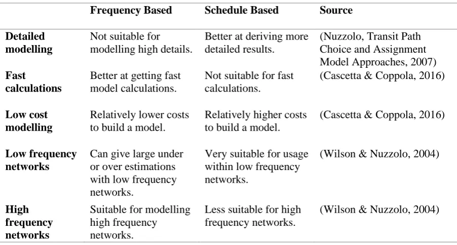
In the table below (Table 1) usage in different situations, according to literature, is described.

Table 1: Differences between methods

Frequency Based Schedule Based Source

Detailed modelling

Not suitable for modelling high details.

Better at deriving more detailed results.

(Nuzzolo, Transit Path Choice and Assignment Model Approaches, 2007) Fast

calculations

Better at getting fast model calculations.

Not suitable for fast calculations.

(Cascetta & Coppola, 2016)

Low cost modelling

Relatively lower costs to build a model.

Relatively higher costs to build a model.

(Cascetta & Coppola, 2016)

Low frequency networks

Can give large under or over estimations with low frequency networks.

Very suitable for usage within low frequency networks.

(Wilson & Nuzzolo, 2004)

High frequency networks

Suitable for modelling high frequency networks.

Less suitable for high frequency networks.

Much fluctuating demands

Cannot cope with fluctuating demands.

Very useful when demand fluctuate very much.

(Cascetta & Coppola, 2016)

Unevenly spaced departure times

Not suitable when departure times are unevenly spread over time.

Very useful when departure times are spread unevenly.

(Cascetta & Coppola, 2016)

Model competition between runs

Cannot model competition between runs since in only looks at sets of runs.

Very useful when competition between runs has to be modelled.

(Nuzzolo & Crisalli, The schedule-based modeling of transportation systems: recent developments, 2009)

Little input data available

Useful when there is a lack of data available.

Not useful since it is required to have much input data.

(Veitch & Cook, 2013)

Long term planning

Less data available of future transit services. Therefore it is very useful.

Less data available of future transit services. Therefore it is not very useful.

(Liu, Bunker, & Ferreira, 2010)

Congested network

Less useful, since it is not able to model individual runs.

It is able to

differentiate between runs, so it is very useful.

(Schmöcker, Bell, & Kurauchi, 2008)

1.3

From the literature it becomes clear that there is a lot of understanding in the improvements a SB approach can provide in theoretical sense. The disadvantages of the SB approach in theoretical sense are also known. In practice, the FB method is still preferred. This preference of the FB method, might be caused by the fact that not much is known about the improvements a SB method brings in practice and if this outweighs the pros of the FB method. Current literature lacks at giving a clear practical comparison between schedule and frequency based approaches. It is not known how large the improvements are and to what extend certain situations need to be modelled with schedule based methods.

The most important disadvantage of the SB method is the costs and performance. The performance depends directly on the detail level that is used in the calculation. The detail level in the SB method can be changed to improve or decrease performance. The perfect balance between a good performance and detailed results in a practical sense is something that does not come forward from the literature.

There is a lack of knowledge about the benefits a SB approach has in practice. This is very important to overcome since there is a demand for the use of a SB approach. Goudappel Coffeng urges to make use of a SB approach in the future. In addition, other public transportation companies have indicated that they would be interested receiving data from a SB method.

1.4

R

A

application and what influences these differences? To achieve this aim the following sub-questions are formulated:

I. What are the main practical differences between both methods? a. What are the differences in input?

b. What are the differences in run-time? c. What are the differences in results?

II. How do the skims of the SB algorithm compare to results from the FB algorithm? a. How do these results behave in different situations?

b. Which algorithm gives results closer to the ground-truth data? c. Are these differences logical?

III. What is the influence of different parameters of the SB algorithm? a. What parameters have large influence?

b. What parameters have the lowest cost benefit ratio?

1.5

R

L

-

In this section the lay-out of this research is described. The study consists of two main parts: an in-depth description of both assignment methods using available literature and a case study done on the Dutch rail network. These main parts are used to reach the aim of this research.

The in-depth description of both methods consists of: an introduction to route assignments, theoretical description of both algorithms and a practical description and application of both methods. More understanding in both methods is gained, by this methodology description. It has to become clear what the main inputs and outputs are. With this information, the first sub-question can be partly answered. This answer is needed to make an application of the assignment methods on the case network possible.

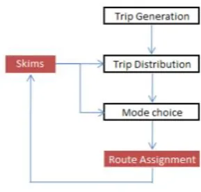
Next, a case is study is done. First, the model and data used in the study is introduced. Then all analysis methods are described, which are used to analyse results of the case network. The case study consists of two main analysis steps. The steps are used to answer the last two sub-research questions. The first step consists of comparing skim results of both algorithms. Subsequently, the third step will be a sensitivity analysis, which gains insights in the results when certain settings are changed. Run-times will also be noted to complete the answer to sub-question one. The steps can be seen in the figure below (Figure 2) and how they contribute to the final goal.

Results of the case study are analysed in the fourth section. From these results and in combination with the theory all research questions can be answered. In the end, the study is discussed and a

2

M

ETHODOLOGY OF

A

SSIGNMENT

M

ETHODS

In this chapter the methodology of the transit route assignment is given, this helps to get more understanding in the topic. Fist some theory about forecasting loads on PT is given. Next, both methods are described in full detail.

2.1

P

Transit route assignments are carried out on a network. Networks must contain all possible origins, destinations and the route options between them. A passenger transportation network is a graph with nodes and links. In the network links are used to model transit lines. Nodes are used to model stops or stations. Centroids can be considered as origins and destinations. All centroids contain data of the destination of travellers. This data is called demand data, it can be found in an matrix. The OD-matrix shows for every centroid the passengers that want to go to any other centroid. To get from the origin centroid to the closest stop at which the transit service can be boarded, an access mode has to be used. To get from the last stop to the destination centroid, an egress mode has to be used. Egress or access modes can be car, bike or walk. An example of a network can be found in Figure 3.

Figure 3: Network with one transit line and three stops (Brands, Romphc, Veitche, & Cook, 2014)

The route assignment, which calculates the proportions of passengers of a route, is part of a four-step model for PT modelling. This model is shown below (Figure 4). The four step model is used to predict the behaviour of travellers. In the first step, trips from every centroid in the network are determined. In the next step, the amount of trips between O and D centroids are calculated. The mode choice determines the mode that a traveller is going to use. In the PT network assignment multiple modes are used, therefore trip mode chains are used (e.g. walk – train – car). The step which is most important in this research and the last step of the 4 step model, is the route assignment. In this step the route between the origin and the destination are determined. A loop can be seen in Figure 4, this is used for iterations. The iterations are done using skims, these are matrices consisting of characteristics of an OD-pair: distance, travel times, costs or a combination of those factors (generalised costs), for each OD-pair (Travel Forecasting Resource, 2019).

The figure below (Figure 4) shows how skims influence trip distribution and mode choice, therefore accurate calculation of skims is very important. Variables of each route are skimmed from the network and put into the skim matrices. When skim calculation of routes is done accurately, it positively influences the entire model. The main part of the skims that determines if a transit service is used is the generalised costs. Generalised costs is a concept that was developed to get one variable that

Figure 4: Four-step model (Veitch & Cook, 2013)

The general scheme of an assignment model in transit modelling can be seen in Figure 5. This scheme consists of a supply, path choice and an supply-demand interaction model. The supply demand and interaction model can be seen as the transit route assignment. As mentioned earlier the two main methods for this are FB and SB. Regularity and information characteristics are gathered by using intelligent transport systems (ITS). This consists of advanced PT systems (APTS) and advances traveller information systems (ATIS). (Nuzzolo, Transit Path Choice and Assignment Model Approaches, 2007)

Figure 5: General scheme of transit assignment models (Nuzzolo, Transit Path Choice and Assignment Model Approaches, 2007)

For this study specifically, train connections are analysed. Most of these intercity, suburban or regional train connections belong to low frequency services (average headways of 15 min or more).

Characteristic for these services, is the assumption that travellers have all information necessary before boarding any transit service. This means that choices about stop and run are made before the trip. Transit services that have a low frequency are also assumed to be uncongested systems. This implies that factors like: vehicle capacity, day-to-day dynamics and the problems that occur with these factors, are not taken into account. (Nuzzolo & Crisalli, The schedule-based modeling of transportation systems: recent developments, 2009)

The attractiveness of routes is determined with the data in the skim matrix. Attractiveness of a route depends on several factors. Less travel time results in more qualitative time-use; less travel time makes a route more attractive. Transfers also have a huge effect on attractiveness of a route. The less

not be too long, since this takes up more time, but it can also not be too short, since this results in more missed connections. The distance a traveller has to walk to the connecting train also determines quality of a transfer. The period in which a transit service departs is also important for the attractiveness of a route. If the transit service departs in the time frame at which the traveller wants to depart, it makes this transit service more attractive. The last factor of attractiveness is the delay that a traveller obtains if it misses the connection. (Guis & Nijënstein, 2015)

2.2

In this part the algorithms used to conduct a frequency or schedule based assignment are described. The methodology of the OmniTRANS assigning method will be explained, specifically the OtTransit method. First, the theory of the algorithm is explained then the practical approach is described. The FB approach is based on (Veitch & Cook, 2013), (Brands, Romphc, Veitche, & Cook, 2014) and (Brands, Multi-objective Optimisation of Multimodal Passenger Transportation Networks, 2015). The SB approach is based on (Friedrich, Hofsäß, & Wekeck, 2001) and (Veitch & Cook, 2013). Both algorithms are implemented in the OmniTRANS software (DAT.Mobility, 2019).

2.2.1 Frequency Based algorithm

It is assumed that an individual traveller is going from an origin O to destination D with a certain mode of PT. This means that the modal split step of travellers has already been completed.

First the stops at which the transit service can be boarded is determined. This is depending on the access or egress mode. The access and egress modes are used to reach the boarding or alighting stop respectively. These modes can be bike, walk or car. For each destination or origin a group of stops is identified which can serve as the start of the PT route. How these stops are selected depends on the following factors:

- Distance radius - Type of PT - Type of stop

- Minimum number of stops

The set of stops that are available is bounded by these parameters. All stops that are selected for the destination or egress stop are possibilities for the final stop. The model that chooses the lines that can be used works in a reversed direction, from the egress stop to the access stop. For every stop on the line that has been identified, the generalised costs are calculated. These generalised costs are the costs to reach destination D, from the moment that the line has been boarded. This excludes the access mode and the waiting time but it includes the egress mode.

The generalised costs are a characteristic of a link in the route. The generalised costs consists of five parts: Travel Distance, Travel Time, Waiting time and Penalty Fare.

These can be calculated with formula 1.

𝐶𝑙𝑖𝑛𝑘 = 𝛼𝑚𝑇𝑙 + 𝛽𝑚𝐾𝑙 + 𝛾𝑚𝑃𝑙 (1) (Brands, Romphc, Veitche, &

Cook, 2014)

Where:

𝐶𝑙𝑖𝑛𝑘 Generalized Link costs of a link

𝑙 Link

𝑇𝑙 On-board Travel time on a link

𝐾𝑙 Fare costs of a link

𝑃𝑙 Penalty for Transfer

When all generalised costs are calculated, these costs are summed up per route. These costs per route are the most important input to calculate the proportion of passengers that use the route. The

probability to board the line is calculated with formula 2.

𝑝𝑙 = 𝐹𝑙𝑒−𝜆𝐶𝑙

∑𝑥∈𝐿𝐹𝑥𝑒−𝜆𝐶𝑙 (2) (Brands, Romphc, Veitche, & Cook, 2014)

Where:

𝐶𝑙 Generalized costs of a line l

𝑥 Any line from stop s reaching j

𝐹𝑙 Frequency of line l

𝜆 Scaling (Logit) parameter

𝑝𝑙 Probability of boarding line l

Since there can be several transit lines at a stop the waiting time used is based on a combined frequency. The combined frequency (CF) is a trade-off between in-vehicle travel time and waiting time. The formula to calculate CF can be found below (formula 3).

𝐶𝐹𝑢= ∑ 𝐹𝑙

𝑒−𝜆𝐶𝑙𝑢

max

𝑥∈𝐿𝑢𝑚𝑒−𝜆𝐶𝑥𝑢

𝑙∈𝐿𝑢𝑚 (3) (Brands, Multi-objective Optimisation of

Multimodal Passenger Transportation Networks, 2015)

Where:

𝐿𝑢𝑚 Subset of lines passing stop u

𝐶𝑙𝑢 Generalised costs of line l from stop u

To calculate the total costs to reach a destination from any origin in the network the formula below is used (formula 4).

𝑇𝐶𝑢= min(𝑀𝑊, 𝑊𝑇) + ∑𝑙𝜖𝐿𝑢𝑚𝑝𝑙 𝑐𝑙 (4)

Where:

𝑇𝐶𝑢 Total costs to reach a certain destination from stop u

𝑀𝑊 Maximum waiting time

𝑊𝑇 Waiting time translated from the combined frequency

2.2.2 Schedule Based Algorithm

In this report the focus will be on the line transit choice, rather than on the stop choice. Only the line choice part of the algorithm will be explained. The input of the algorithm is a temporal distribution of the travel demand between origin and destination (DEM). This temporal OD-matrix distribution is then further spread in equally divided time steps. These time steps define the moment at which travellers are placed on the network. If the time step gets smaller, the calculation gets more detailed and the computation time will be longer.

To obtain a set of routes that a traveller from O to D a branch and bound method is used. First all connection segments between O and D are determined. A route from O to D that is made up of a train that goes from O to T (transfer stop) and a train that goes from T to D, consists of two connection segments. Subsequently, the arrival and departure times of these connection segments are stored in a sorted array.

to D. From this tree, the paths are determined and are used in the choice of routes. The levels that can be seen in the figure represent the transfers in the path. The amount of transfers can be limited by setting the maximum interchange setting. In the example figure below, this limit has been set to four.

Figure 6: A Connection Tree (Friedrich, Hofsäß, & Wekeck, 2001)

It is assumed that travellers make their decision based on the generalised costs. These costs are a combination of the perceived journey time (PJT), the transit fare (FARE) and the difference between the real and preferred departure times. A way to calculate the PJT of a connection c is shown in formula 5. The generalised costs of connection c can be calculated with formula 6.

𝑃𝐽𝑇𝑐 = 𝐽𝑇𝑐+ 2 𝑇𝑇𝑐+ 2 𝑁𝑇𝑐 (5) (Friedrich, Hofsäß, & Wekeck, 2001)

𝐶𝑐= 𝑞1 𝑃𝐽𝑇𝑐+ 𝑞2 𝑈 𝑐 (𝑎)+ 𝑞3 𝐹𝐴𝑅𝐸𝑐 (6) (Friedrich, Hofsäß, & Wekeck, 2001)

Where:

𝑈𝑐 (𝑎) Temporal utility for travellers departing in time interval a

𝑞1,2,3 User set constants

𝐽𝑇𝑐 Journey time

𝑃𝐽𝑇𝑐 Perceived journey time

𝑇𝑇𝑐 Transfer time

𝑁𝑇𝑐 Number of transfers

The temporal utility shows the difference between a passengers real and preferred departure time. When the connection departs within time interval a, 𝑈𝑐 (𝑎) will be zero. If the connection departs at

another time U will increase monotonously. U cannot become negative, since travellers cannot depart before their preferred departure time interval.

The proportion of travellers using a connection is calculated with a utility function, which takes into account the ‘independence’ of a connection. Independence of transit lines is defined as the amount of difference between two transit lines. The difference is based on departure and arrival time, perceived journey time and fares. Formula 7 is used to calculate the independence of a connection c, which is part of subset C (𝑐 ∈ 𝐶).

𝐼𝑁𝐷𝑐=

1

∑_{𝑐′∈𝐶}𝑓_{𝑐(𝑐′)}=

1

1+∑_{𝑐′≠ 𝑐}𝑓_{𝑐(𝑐′)} (7) (Friedrich, Hofsäß, & Wekeck, 2001)

𝑓_𝑐(𝑐′₎= (1 −

𝑥_{𝑐(𝑐′)}

𝑠𝑥 ) × (1 − 𝛾 × 𝑚𝑖𝑛 {1,

𝑠𝑧 |𝑦_{𝑐 (𝑐′)}|+𝑠𝑦 |𝑧_{𝑐(𝑐′)}|

𝑥_𝑐(𝑐′₎=(|𝐷𝐸𝑃𝑐−𝐷𝐸𝑃𝑐′|+ |𝐴𝑅𝑅𝑐−𝐴𝑅𝑅𝑐′|)

2 (9)

𝑦_𝑐(𝑐′₎= 𝑃𝐽𝑇_𝑐′− 𝑃𝐽𝑇_𝑐 (10)

𝑧_𝑐(𝑐′₎= 𝐹𝐴𝑅𝐸_𝑐′− 𝐹𝐴𝑅𝐸_𝑐 (11)

Where:

𝑓𝑐 An non-negative evaluation function

𝑥_𝑐(𝑐′₎ Temporal similarity of connection c

𝑦_𝑐(𝑐′₎ The advantage of connection c considering PJT 𝑧_𝑐(𝑐′₎ The advantage of connection c considering FARE 𝑠𝑥,𝑦,𝑧 Determine the range of influence for the three variables

𝛾 Global parameter

𝐷𝐸𝑃 Departure time

𝐴𝑅𝑅 Arrival time

The evaluation function gives penalties to connections with departure times that are close to each other. This means that connections that are identical or have similar departure times are assigned a low ‘independence’. Goal of the function is to spread travellers realistically over all different connections. Connections that are similar or identical attract passengers from the same group, which results in lower usage, whereas connections that are unique also attract passengers from a unique group.

The last factor that is necessary to compute the proportion of passengers on a certain connection is a Box-Cox transformation, which is calculated with formula 12.

𝑏𝑡(𝐶(𝑐)) = {

𝐶(𝑐)𝑡−1

𝑡 𝑖𝑓 𝑡 ≠ 0

log(𝐶(𝑐)) 𝑖𝑓 𝑡 = 0

(12) (Friedrich, Hofsäß, & Wekeck, 2001)

Where:

𝑏𝑡(𝐶(𝑐)) Box-Cox transformation of generalised costs of route c

Now the proportion of passengers on each connection can be calculated, this is done with formula 13.

𝑃𝑎(𝑐) =

𝑒−𝛽 ∙ 𝑏𝑡(𝐶𝑐)∙ 𝐼𝑁𝐷_𝑐

∑_{𝑐′∈𝐶}(𝑒−𝛽 ∙ 𝑏𝑡(𝐶𝑐)∙ 𝐼𝑁𝐷_𝑐) ∙ 𝐷𝐸𝑀(𝑎) (13) (Friedrich, Hofsäß, & Wekeck, 2001)

Where:

𝑃𝑎(𝑐) Proportion of passengers on route option c from stop a

𝛽 Logit parameter

𝐷𝐸𝑀(𝑎) Demand for access stop a

This makes it easier to show the effect of the concept of independence. Assume a scenario in which DEM(a) = 100. These 100 passengers can make use of a few connection between a = [08:00, 09:00].

All transit connections depart within a, therefore the assumption is made that Ua (c) = 0. To make it

easier q1 and q2,3 are assumed to be 1 and 0 respectively. fc is used as evaluation function. To get the

standard Kirchhoff distribution, β and t are assumed to be 2 and 0 respectively.

Table 2: Connection split: three connections with fixed headway (Friedrich, Hofsäß, & Wekeck, 2001)

c DEP(c) PJT(c) IND(c) Pa(c) not using IND(c) Pa(c) using IND(c)

1 08:15 20 min 1,00 33 33

2 08:30 20 min 1,00 33 33

3 08:45 20 min 1,00 33 33

A second example is shown below (Table 3). In this example, it becomes clear that identical connection get the same proportion by using the independence.

Table 3: Connection split: adding an identical connection (Friedrich, Hofsäß, & Wekeck, 2001)

c DEP(c) PJT(c) IND(c) Pa(c) not using IND(c) Pa(c) using IND(c)

1 08:15 20 min 1,00 25 33

2 08:30 20 min 0,50 25 16,5

3 08:30 20 min 0,50 25 16,5

4 08:45 20 min 1,00 25 33

Another example shows the effect of the insertion of a fast connection (Table 4). As can be seen from the table, the fast connection only has a small effect on the first connection, since it departs much later than connection one. The fast connection departs close to connections two and four, therefore it detracts more passengers from these connections.

Table 4: Connection split: adding an fast connection (Friedrich, Hofsäß, & Wekeck, 2001)

c DEP(c) PJT(c) IND(c) Pa(c) not using IND(c) Pa(c) using IND(c)

1 08:15 20 min 1,00 21 23

2 08:30 20 min 0,86 21 19

3 08:40 15 min 0,94 37 39

4 08:45 20 min 0,86 21 19

2.3

In this part the practical approach is described. To start with, the settings and parameters are explained. Subsequently, a case is used to describe the methodology of both methods.

2.3.1 Logit parameter

The logit parameter has to be defined for both methods and is used to control the difference between less optimal and optimal routes. A high logit parameter value means that a larger proportion of the travellers make use of the most optimal route option. If it becomes smaller a larger proportion uses the less optimal routes. This process is shown in Figure 7. Line A is the most optimal line and line B is a less optimal line. In reality these very low logit values are never used, since sub-optimal routes are never preferred over optimal routes.

2.3.2 Frequency Based configuration

Since demand varies during the day, FB assignments are done over a certain time period (e.g. morning rush hour). The OD demand matrix of this specific time period is then used in the assignment.

Bounding settings are used to determine maximum skim values, to prevent the methods from computing unrealistic skim values. For the FB method the maximum access waiting time and

maximum transfer waiting time can be defined. These settings are used to prevent extreme unrealistic waiting times at low frequencies. The maximum transfer waiting time also makes it possible to model short transfer times, which were otherwise impossible.

2.3.3 Schedule Based configuration

Level of detail can be controlled to keep control of computation times. Time step and route choice set size can have great influence on the computation times. Size of time steps determines the smallest level of time that the SB method is able to differentiate in. A smaller differentiation level means more detailed modelling, but also more computation time. Size of route choice set determines the amount of possible routes options between O and D. Large sets of routes mean a lot of possibilities and therefore higher details and more computation time. It is possible to ignore certain unlikely route options in the route choice set to improve computation times.

It is possible to limit the route choice set in the SB assignment by using branch and bound parameters. There are three branch and bound parameters: cost limit, travel time limit and transfer limit. The cost limit and travel time limit parameters are used to define the maximum relative difference that a route option is allowed to have, compared to the most optimal solution. Assume a scenario where the cost limit parameter is set to 1,3. In this scenario, route options are only accepted if it costs less than 1,3 times the cost of the most optimal solution. The transfer limit parameter defines the maximum absolute difference in transfers, compared to the most optimal solution.

For the SB method it is also possible to set a limit on the access waiting time and the transfer waiting time. Since passengers want to depart in their designated timeframe, only routes within a defined time frame are selected using the maximum access waiting time setting. In a scenario where the person wants to leave only 30 minutes after its desired departure time, only routes within that timeframe are considered. For example, if the person wants to leave at 07:00, only routes that before 07:30 are considered. It does not matter if the routes within that time interval are less optimal. If the algorithm is not able to find any route that meets all settings and is within the desired time period, travellers are moved to the subsequent time step. The maximum interchange waiting time setting limits possible routes to a certain maximum transfer wait time.

2.3.4 Application

Assume a scenario in which a group of travellers arrive at station A between 07:20 and 07:25 and want to travel to B. For this route there are two options that are logical to use, the options can be found in the table below (Table 5).

Table 5: Options for a single time slot

Option Type Departure time

Average Access Waiting Time (minutes)

In-vehicle Time (minutes)

Option 1 Sprinter 07:24 0 68

Option 2 Intercity 07:46 25 57

When running a SB assignment the outcome is that 50% of the travellers use the sprinter connection and the other 50% uses the intercity connection. The calculated skim value for travel time of the simulated time slot is 62,5 minutes, this is the result of this assignment.

It is possible to see the proportion of travellers per route option. For the FB method, it is only possible to differentiate between route types, not between runs. To get the same result from the FB assignment the skim values have to be examined. From skim matrices, it can be concluded that the Intercity connection is used approximately 65% and the Sprinter 35%. However, these proportions are

calculated using a load for the entire morning rush hour period (07:00 – 09:00), unlike the single time slot that is used for the SB assignment. The FB method is also not able to simulate a single small time slot.

To model a larger period like in the FB approach for the SB method the simulation period has to be larger. The simulation time needs to contain all possible options to create the most realistic simulation. The simulation time is one hour. The same origin-destination pair will be simulated, but now with passengers departing at every time between 07:00 and 08:00. The time step setting is still set to five minutes. This will result in 12 time steps of five minutes. In each time step an equal amount of passengers are put on the network.

Assume that a group of travellers arrive at station A between 07:00 and 08:00 and want to travel to B. All logical options are shown below (Table 6).

Table 6: Options for assignment over entire hour

Option Type Departure time

Average Access Waiting Time (minutes)

In-vehicle Time (minutes)

Option 1 Intercity 07:16 8 57

Option 2 Sprinter 07:24 12 68

Option 3 Intercity 07:46 15 57

Option 4 Sprinter 07:54 15 68

Option 5 Intercity 08:16 23 57

Option 6 Sprinter 08:24 27 68

Waiting times are determined as an average over the time steps. This is due to the fact that for every time step a skim value for waiting time is calculated. These waiting times are an average for all time steps between the departure time of this specific train and the departure time of the last train of the same type.

Table 7: Results for SB assignment

Option Type Proportion

Option 1 Intercity 33%

Option 2 Sprinter 4%

Option 3 Intercity 46%

Option 4 Sprinter 5%

Option 5 Intercity 12%

Option 6 Sprinter 0%

3

C

ASE

S

TUDY

In this chapter the case study used to gain results is described. First, the model and data used in the case study is described. Subsequently, the analysis methods are described.

3.1

D

N

R

M

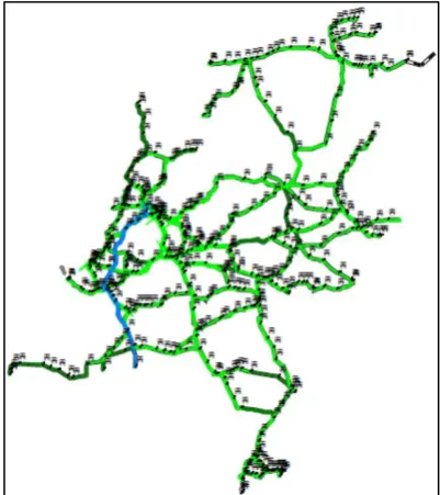
The first step of the research involves gathering data to work with. The most important model that is used is the Dutch National Rail Model, further revered to as National Rail Model. This is a network of all train lines and stations in the Netherlands in 2013. An overview of the network can be seen in the figure below (Figure 8). Within this network, all input variables for: schedule, frequency and demand, are already defined. Timetables and frequencies correspond with the real schedule at that time. The network has 402 centroids, which can be seen as stations. Each station can be seen as origin or destination, therefore there are 161.608 OD-pairs. All used data from the network also consists of 161.608 data points. OD demand data is calibrated from the station exit and entry data, which is derived from (Treinreiziger.nl, 2019), the structure is based on the national model from 2008. Demand data is separated in three time periods: morning rush hour, evening rush hour and ‘rest day’. The software that is used to run the models is OmniTRANS 8.0 (DAT.Mobility, 2019) this software is suitable for the simulation of low-frequency transit systems according to: (Nuzzolo & Crisalli, The schedule-based modeling of transportation systems: recent developments, 2009).

Figure 8: Overview of the National Rail Model

3.2

‘

’

3.3

S

Both methods are compared using skim matrices. These skim matrices consist of characteristics of each OD-pair. The skims can be separated in four categories: total route, access, in-vehicle and egress. For each category skims for travel time, waiting time and transfer penalty are used in the comparison. Skims are generated using both algorithms.

The assignments are done using both algorithms. Skims are generated per OD-pair. To make comparison possible, skims of both methods have to represent the same time period. The morning peak period between 07:00 and 09:00 is used. This means that the OD demand matrix, schedule and frequency of this time period is used in the assignment.

The SB assignment is done over a 60 minutes period: from 07:00 till 08:00. In the dutch rail network all lines depart at least once an hour, this means a 60 minute period includes all possible options. Demand fluctuation over the time period was not used, this was done to make comparison with FB data easier. Another reason to not implement demand fluctuation is that there is no information available to implement this. Since the demand fluctuation was disabled, the entire 60-minute period represents 100% of the demand in the morning rush hour. The 60 minute time period is spread in twelve, five minute time steps.

Maximum access and transfer waiting time for the FB assignments is set to 60 and 30 minutes respectively. For the SB assignment both were set to 30 minutes. The FB assignment works with average waiting times, therefore the SB and FB limits give comparable results with these settings.

The logit parameter value that is used is 0,6. This parameter is based on earlier studies carried out at Goudappel Coffeng. This setting of the logit parameter is used for both methods. Some travellers make use of sub-optimal routes, but the most travellers still make use of the most optimal route with this logit value.

In order to compare the FB skim matrices with the SB skim matrices the unit has to be equal. Skim results for the SB method are built for every time step. In a standard situation, every OD-pair has skims for every time period. For the FB method, results are an average of the whole assignment period. Therefore the skims of all time periods of the SB method have to averaged. With the average results of the SB assignment it is possible to compare with FB skim results.

During the skim generation it also became clear that for some relations only a few time steps had useful results. When the algorithm is not able to find any route within that time step, the skim results are not useful anymore. Useless skims are called ‘disconnected’ skims and useful skims are called ‘connected’ skims. There can be multiple reasons for these disconnected skims. It is possible that no route can be found within the maximum access waiting time. Another possibility is that there are only routes available with a transfer wait time higher than the maximum allowed transfer wait time. An average of the SB skims can only be created when these skims are filtered out of the data. In the normal situation, all time steps are considered in averaging the skims, in reality only the connected skims were used in the calculation.

3.4

S

This method is used to answer the following sub question: How do the skims of the SB algorithm compare to results from the FB algorithm? To answer this question skim results of both algorithms are compared. Skim matrices of travel time, waiting time and penalty are used in the comparison. The skim data is analysed both in-depth and quantitatively.

3.4.1 Quantitative analysis

The quantitative analysis and comparison is done using the entire skim matrix. This means that all relations are considered, unless they do not meet the minimum skim number. Generated skim matrices from the FB assignment are subtracted from the SB skims. The median is used in this case, instead of the average, to filter out all extreme results. This median difference is then used to make histograms. These histograms help to create a better overview of the large data set. Skims types that are analysed are: in-vehicle travel time, total travel time, total waiting time, access waiting time, transfer waiting time and penalties.

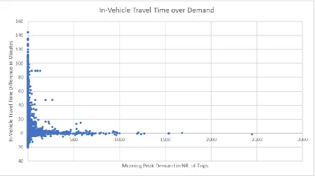
It is also valuable to know if important relations behave as expected. Important relations are defined as relations that have large demands. The in-vehicle travel times are compared with the demand matrix to verify if the method gives reliable results for important relations. A scatter plot is made to show to what extend high demand relations have high deviations.

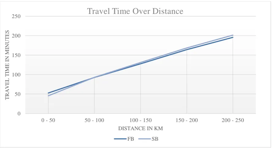
The next analysis that will be done is a characteristics based analysis. OD-relation skim values are divided based on their characteristics. Characteristics that are used in the comparison are distance and number of transfers. OD-relations are put into groups with the same characteristics, however, only if they meet the characteristics for both the SB and FB assignment results. Median values from the groups are put into a graph and are then used to analyse the results. The focus will be on finding correlations between certain situations. These situations are important since it makes clear in what situations which method is better to use.

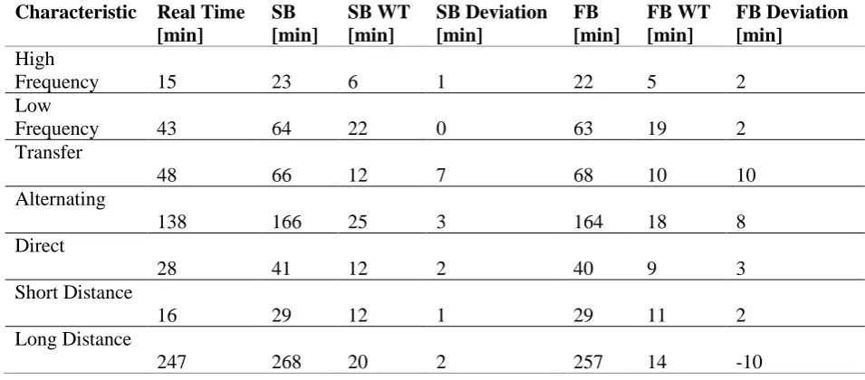
3.4.2 In-depth analysis

An in-depth analysis is done for some random OD relations with specific characteristics. These relations are handpicked from the network. For every unique situation a few relations are observed. These situations are: high frequency, low frequency, no-transfer, with transfer, alternating (transfer/no-transfer), short distance and long distance. The alternating situation exists when a path between O and D differs over time. This means that at some time in the hour a direct connection to the destination is possible and at another time a transfer is required.

Travel time, waiting time and penalty skim data of both algorithms is used in the analysis. The skim values that have been gathered from the real world network, are also used to check if they correspond with reality. This is done by using the real world travel time data from the NS application. The differences in certain situations are then logically explained. An analysis like this creates more in-depth understanding of the benefits of the SB method.

3.5

S

Parameters that are tested need to be specific for a SB assignment and influence the detail level. Parameters that meet these requirements are: time step size, branch and bound, maximum number of transfers and maximum access waiting time. Since the effect of disconnected skims is also something which can have large influences, this parameter is also tested.

In the table below (Table 8), the branch and bound parameters that are used in the sensitivity analysis are shown. As already mentioned, the branch and bound parameters define the routes that can be used by the travellers between O and D. Strict settings only allow routes that are slightly less optimal than the most optimal route between O and D. Loose settings allow very sub-optimal routes to be used. The loose extra settings also allows routes with two extra transfers.

Table 8: Branch and Bound Settings

Settings Name Allowed extra costs

Allowed extra time

Allowed nr. of extra transfers

Strict 10% 20% 1

Middle 20% 30% 1

Loose 30% 50% 1

Loose Extra 30% 50% 2

All settings, for every sensitivity analysis that is performed, can be found in Table 9. The parameter settings for times step size are changed from high detailed, small steps, to lower detailed, larger steps. Maximum number of transfer settings are changed from a very low limit, to a very high limit. The low limit only allows routes with a two transfers and the high limit allows routes with a large amount of transfers. The settings for maximum access waiting time are changed from a very low waiting time, to a very high waiting time. Only short access waiting times are allowed for low access waiting time settings and long waiting times for high access waiting time settings. Minimum number of skims settings are changed from a low limit to a high limit. A low limit considers all OD-pairs with at least one useful skim. High limit settings only consider the OD-pairs of which all skims are useful.

For each calculation in the sensitivity analysis, computation time is noted. When the skims are generated, the improvements in skim results are determined. In this way, the pros (more detailed results) of the SB method are plotted against the cons (higher computation time). Then the perfect balance between computation times and result improvement can also be found.

Table 9: Settings sensitivity analysis

Test Nr.

Time Step Size (min)

Branch and Bound

Max. Nr. of Transfers

Max. Access Wait Time (min)

Nr. of Skims

1 1 Strict 2 15 >0

2 2 Middle 3 30 >5

3 5 Loose 4 60 >11

4 10 Loose Extra 5 120 -

5 15 - - - -

4

R

ESULTS

In this chapter all results are given. Results are given per type of analysis and all results are analysed and discussed.

4.1

S

In this part, the skim results from the National Rail Model are used. Skim results are gathered using both methods. The results from the National Rail Model represent a real world situation, these are more valuable than the results from the test network. Results from the test network can be found in appendix C (C. Test network results). The settings of the skim generation can be found in appendix B (B. Settings). In appendix F (F. Amount of Connected skims) the amount of skims for the used SB dataset can be found.

4.1.1 In-Vehicle Travel Time

Results of the in-vehicle travel time comparison can be found in this section.

Figure 9: Histogram In-Vehicle Difference

The graph above (Figure 9), shows the relative difference for in-vehicle travel times. As can be seen from the graph, frequencies are a lot higher at the positive side. The median difference is 4,2%. It can be concluded that in vehicle travel times of the SB assignment are higher on average. Less optimal routes can become the best option when demand is equally spread over the entire hour, this can cause the higher in-vehicle travel time. For example: the SB method makes it possible that travellers arrive only minutes after the most optimal route has departed. These travellers are much less likely to make use of the most optimal route, because of the longer waiting time. In a FB assignment the preferred time of departure is not taken into account, therefore it is much more likely the optimal route is used by this method.

The accuracy of the difference can be seen in the table below (Table 10). The table shows the

percentage of results that are within a certain difference interval from 0%. For example: 51% of all SB in-vehicle travel times deviate ±5% from the FB in-vehicle travel times. From this data, it can be seen that there is a significant difference between both in-vehicle travel time skims. However, most results only have a small difference.

0 5000 10000 15000 20000 25000 30000 35000 40000 45000 50000

F

re

qu

ency

Relative Difference

Table 10: Accuracy of Results

Interval Percentage of results

±5% 51%

±10% 71%

±15% 82%

±30% 96%

From the scatter plot below (Figure 10), the demand that belongs to a certain difference is shown. As can be seen, most high demand results are located on the line of zero difference. It can be concluded from the graph, that most high-demand relations only have a very small deviation. Most large deviations can be found in less used OD relations. The same scatter plot but with a travel time difference expressed in percentage can be found in appendix H (H. Relative Scatter Plot In-Vehicle Comparison).

Figure 10: In-Vehicle Travel Time Difference over Demand

4.1.2 Total travel Time

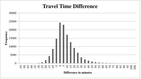
Figure 11: Histogram Total Travel Time Difference

Table 11: Relative Difference of Travel Times

Interval Percentage of results +30% 58%

+15% 49% +10% 39% +5% 22% -5% 21% -10% 34% -15% 39% -30% 41%

4.1.3 Waiting time

Subsequently, the results of the waiting time comparison are given. First, the total waiting time difference histogram is given. Total waiting time consists of two elements: access and transfer waiting time, both elements are also analysed. The histograms of access and transfer waiting times are given in appendix D (D. Waiting time results).

As can be seen from Figure 12, the frequencies are slightly higher at the left side of the graph. This means that waiting times are lower for the SB assignment. The median difference is -2,1 minutes. In the table below (Table 12), percentage of results that are within a certain difference interval from 0% can be seen. Percentages in the table also show lower travel times for the SB assignment. To find out where the differences come from the component skims are also analysed.

Since the access waiting time is a part of the total waiting time, access waiting times can possibly explain the results from the total travel time. The median of the difference in access waiting time is 0,5 minutes. From the median, it be seen that the SB access wait time is slightly higher. This might be caused by the perfect distribution of a FB assignment. The SB assignments assigns travellers every time step, therefore the size of the time steps influence the access waiting time. With a FB assignment, travellers receive an average waiting time based on an equal distribution over the time period.

Overall, the waiting time is lower for a SB assignment, therefore it cannot be caused by the access 0 5000 10000 15000 20000 25000 30000 -5 5 -5 0 -4 5 -4 0 -3 5 -3 0 -2 5 -2 0 -1 5 -1

0 _-5 0 5 _{10 15 20 25 30 35 40 45 50 55 60 65 70 75 80 85 90 95}

1 0 0 2 0 0 F re qu ency

Difference in minutes

waiting time. In appendix D.1 (D.1 Access waiting time) a full analysis of the access waiting time can be found.

The transfer waiting time is also part of the total waiting time. It became clear that the access wait time was not responsible for the lower total waiting times for a SB assignment, therefore the transfer waiting time must be responsible for this result. The median of -3 minutes, clearly shows a lower waiting time for transfers. In appendix D.2 (D.2 Transfer waiting time) a full analysis of the transfer waiting time can be found. It becomes clear that the transfer waiting time is the reason for the lower total waiting times for a SB assignment. This is caused by the more detailed calculation of the transfer waiting time by the Sb method. Most transfers are the Dutch rail network are synchronised, which means that very short transfers are guaranteed. The FB assignment is not able to calculate these transfer times exactly, instead it is only able to give an average waiting time based on the frequency. With the SB assignment, the short transfer time can be modelled.

Figure 12: Histogram Waiting Time Difference

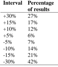
Table 12: Relative Difference of Waiting Times

Interval Percentage of results +30% 27% +15% 17% +10% 12% +5% 6% -5% 7% -10% 14% -15% 21% -30% 42%

4.1.4 Penalties

To get more insight in the way penalties are assigned with both methods, the difference between penalties is also analysed. Differences are shown in the histogram below (Figure 13). The histogram clearly shows a deviation to the left. From the deviation, it can be concluded that there are less penalties given for a SB assignment. But, as can be seen, the difference is very small. Most relations

0 5000 10000 15000 20000 25000 30000 -6 5 -6 0 -5 5 -5 0 -4 5 -4 0 -3 5 -3 0 -2 5 -2 0 -1 5 -1

0 _-5 0 5 _{10 15 20 25 30 35 40 45 50 55 60 65 70 75}

F

re

qu

ency

Difference in minutes