Dynamics of state feelings : State Affect: A longitudinal study with the use of experience sampling

1

Dynamics of state feelings

State Affect: A longitudinal study with the use of

experience sampling

Bachelor Thesis

Negar Sadeghi Hassanabadi (1761188)

27.06.2019, Enschede

University of Twente

Department of Positive Psychology & Technology

First supervisor:

Dr. P.M ten Klooster

2

Abstract

Background: Feelings vary over time, they are not stable but are often measures as trait-like

concepts. Recently, researchers have raised their interest in finding ways to measure state feelings

and moods of people. Experience Sampling Method (ESM) is a method that is often used for

momentary assessments of feelings or behaviors. In contrast to cross-sectional designs, it allows

us to measure feelings, the moment they occur and therefore allows for a broader understanding of

participants emotional life. Russel and Watson & Tellegen (1985) suggested that feelings are not

discrete entities rather they are dimensional. Alexithymia refers to people who have difficulties to

define or differentiate between their feelings. Surprisingly 1/5 of the general population shows

signs of alexithymia. Objective: The aim of this study was to get an impression of the dynamic of

state feelings with the use of experience sampling. Another aim was to assess whether ESM is

suitable for measuring state feelings. A different aim was to investigate whether there are

differences in state and trait feelings of people who show or not show signs of alexithymia.

Method: The sample was derived from a non-clinical young population, with the age between 18

and 30 years. Either being students or full-time employees. In a longitudinal ESM study, the

relationship between state and trait feelings was measured. The participants were asked to fill out

the affect grid via the TiiM application for seven days four times a day at specific time points. At

the eight-day participants were asked to fill out the Positive and Negative Affect Scale (PANAS)

and Toronto-Alexithymia Scale 20 (TAS20). Results: A series of Linear mixed model (LMM)

analyses were conducted. State pleasure significantly covariates with the positive affect of the

PANAS. A significant main effect for the negative affect of the PANAS and state pleasure was

found. A strong significant negative correlation between the level of pleasure of participants and

the negative affect of participants was found with a post-hoc analysis. For the TAS20, it was shown

that pleasure and energy scores of participants with signs of alexithymia are strongly positively

correlated, in contrast to the scores of pleasure and energy of participants without signs of

alexithymia. Scores of PA and NA affect of the PANAS and their state pleasure strongly positively

correlate as well. Scores of NA affect of the PANAS and pleasure scores of the affect grid of

participant’s without sings of alexithymia do significantly and strongly correlate. Conclusion: It

was found out that state feelings do vary over time and that ESM is a valid method to measure state

feelings because, in this study, trait and state feelings do correlate but not too strong, suggesting

3

found that participants who have signs of alexithymia have difficulties differentiate between

pleasure and energy, as well as positive and negative affect.

Introduction

Feelings and Mood differ. They differ not just within populations but also within persons

themselves. There are a spectrum of feelings and moods people can feel and the dynamics make it

possible for them to change not only within the day but also within seconds (Watson & Clark,

1984; Kuppens, Stouten, & Mesquita,2009). Research in psychology regarding mood has a long

tradition. It is not only interesting to investigate them because it underlies a variety of psychological

disorders or corresponds to a part to personality characteristics but also because humans experience

them in a wide spectrum within a day (Tellegen, 1985; Watson & Clark, 1984); Kuppens, Stouten,

& Mesquita,2009; Ebner-Priemer, Eid, Kleindienst, Stabenow, & Trull, 2009). It is a highly

discussed topic, and therefore, there are many opinions and theories, aimed to explain underlying

mechanisms (Tellegen, 1985; Watson & Clark, 1984; Russel, Weiss, & Mendelsohn, 1989;

Kuppens, Oravecz, & Tuerlinckx, 2010).

There are several frameworks by which psychologists classify emotions, feelings, and

moods. These can be classified into two fundamental viewpoints. The first one proposes that

emotions are discrete and fundamentally different constructs. It is originated from Darwin (1872)

and based on this Tomkins (1962), proposed that emotions and moods are products of evolution

and genetically determined. Tomkins argues that they are distinguishable not only on the basis of

their neural features but also on behavioral and expressive features. His views influenced the work

and ideas of Paul Ekman and Carrol Izard, who are known for their theory of discrete emotions

(Colombetti, 2009). It has to be acknowledged that the limitations of this approach progressively

became apparent. Researchers found out that measures of different affects are not as discrete as

supposed, rather they are strongly and systematically interrelated (Watson & Clark, 1997).

Thus, researchers started to assume that affects are not discrete, rather they are dimensions,

thus creating the second viewpoint. The dimensional models of emotions underlie the hypothesis

that a common and interconnected neurophysiological system is responsible for all affective states

(Russel, 2009). Many of the commonly used frameworks of affect belong to the second viewpoint

4

dimensions, pleasurable versus un-pleasurable, arousing or subduing, and strain or relaxation. In

order to conceptualize human emotions, dimensional models of emotions define where they lie in

two or three dimensions. Since then deprived of evidence, a general consensus has been made that

two broad factors are incorporated in the dimensions of affect. Thus, nowadays most models

incorporate valence and arousal or intensity dimensions (Watson & Clark, 1997). The most

commonly used models are the circumplex model (Russel, 1980), and the Positive Activation –

Negative Activation (PANA) model by Watson and Tellegen (1985) (Rubin & Talarico, 2009).

The circumplex model, developed by Russel (1980), suggests that emotions are

operationalized in a two-dimensional circular space, containing arousal and valence dimensions.

The horizontal axis represents valence while the vertical axis represents arousal. The center of the

circle presents a neutral valence and a medium level of arousal (see Figure 2). Russel (1980)

describes his model as representative of core affect, which consists of the most elementary feelings

that are not necessarily directed toward anything. Essentially, it is how we feel at a particular point

in time. Researchers have suggested that core affect is fundamentally a combination of two types

of feelings continuums; Valence (pleasant to unpleasant) and arousal (low to high arousal) (Russel,

1980). Within the years the term arousal has been replaced by energy (low to high energy) (Schutz, Quijada, De Vries, & Lynde, 2010). Accordingly, Russel (2009) describes core affect as a "pre-conceptual primitive process, a neurophysiological state, accessible to consciousness as a simple

non-reflective feeling: feeling good or bad, feeling lethargic or energized". He further elaborates

on the continuum which incorporates two types of feelings, stating that core affects although being

two dimensional, is subjectively perceived as a single feeling. This means that when combining

the two dimensions with each other, the result is a unified feeling. For example, being high in

energy while experiencing high unpleasantness results in being tense. Core affect, although it can

account for a broad range of emotional states and provides a solid basis for discussing similarities

and differences among affective states, is not the same as emotions, and is more similar to moods

(Russel, 2009). Different types and intensities of feelings and moods can be experienced,

depending on the quality, intensity, and content of the individual's experience on the

above-mentioned dimensions (Plass & Kaplan, 2016). In order to test his circumplex model theory Russel (1980) introduced the affect grid which was designed to assess two dimensions of affect,

pleasure-displeasure, and arousal-sleepiness. It is suitable for any study that requires judgments of affect of

5

that is short and easy to fill out and, therefore could be used rapidly and repeatedly. It has been

proven to be a valid instrument to assess mood (Russel, 1980).

The PANA model, invented by Watson and Tellegen (1985), does not specifically

incorporate arousal. Instead, it suggests that positive and negative affect are two separate systems.

This is due to the fact that the PANAS is based on an orthogonal rotated variant of the

pleasure-arousal scale, which has shown that positive and negative moods are largely independent of another

(Watson & Tellegen, 1985). States of higher arousal tend to be defined by their valence and states

of lower arousal tend to be more neutral in terms of valence. Positive affect (PA) reflects the extent

to which a person feels enthusiastic, active and alert. Thus, high PA is a state of high energy, full

concentration and pleasurable engagement whereas low PA is characterized by sadness and

lethargy (Watson & Tellegen, 1985). Contrasting to this, negative affect (NA) is a general

dimension of subjectively perceived stress and un-pleasurable engagement with a variety of

aversive mood states, with low NA being a state of calmness and serenity (Watson & Tellegen,

1985). It has to be highlighted, that the model of Watson and Tellegen (1985) has been the more

prominent scale for measuring mood and has been used far more often than the circumplex model

of Russel (1980). Hence, it has been far more often validated and there are different reliable and

valid versions of the PANAS. In contrast to that, the affect grid has not been used that often

although it provides a valid and reliable measurement for mood.

Particularly, but not exclusively, researchers have raised their interest towards moods

because many psychological disorders express themselves with a variety of moods and

fluctuations, called mood disorders (Solomon, Leon, Coryell, Endicott, Fiedorowicz, & Keller, 2010; Kessler, Avenevoli, & Merikangas, 2001; Ebner-Priemer, Eid, Kleindienst, Stabenow, & Trull, 2009). Until now, most of the research concerning moods or feelings have focused on it as a trait-like concept (Watson & Tellegen, 1985; Kuppens, Stouten, & Mesquita, 2009; Scherer,

2000).

A trait is defined as a more permanent presence and a stable level of emotion. It refers to

the stable, consistent and enduring disposition of the individual, including emotional reactions

and temperament, rather than situational, variable and temporary factors. On the opposite, a State

refers to a temporary emotional fluctuation, which is a momentary emotional reaction to internal

and/or external triggers. It evolves physical, behavioral, cognitive and psychological reactions

(Zelenski & Larsen, 2000). Feelings as a state are not stable, they can change from moment to

6

this is typically the case, such as bipolar disorders and depressive disorders. This is due to the fact

that people with those disorders most of the time have a general emotional state or mood which is

distorted or inconsistent with the circumstances that they are in. Thus, interfering with their

ability to function (emotions (Taylor, Ryan, & Bagby, 1985; Munoz 1995).

Moreover, many people who suffer from mood disorders display alexithymia. Alexithymia

refers to difficulties in perceiving and describing the emotions of others and themselves (Taylor,

Ryan, & Bagby,1985; Gross & Munoz, 1995; Linehan, 1993). The core characteristics of alexithymia are marked dysfunction in emotional awareness, social attachment, and interpersonal

relating. Furthermore, individuals suffering from alexithymia also have difficulty in distinguishing

and appreciating the emotions of others, which is thought to lead to un-empathic and ineffective

emotions (Taylor, Ryan, & Bagby, 1985). One aspect to consider is that 18% of the general

population have difficulties in verbalizing and expressing their emotions or the emotions of others

(Mattila et al. 2006). Thus, it is important to check if participants display symptoms of alexithymia

while measuring mood or feelings. In this study, it is hypothesized that participants who have signs

of alexithymia have difficulties differentiating or maybe even confuse their daily mood and thus

their levels of pleasure and energy, should either be the same or totally different. Likewise, it is

assumed that they have difficulties differentiating between positive and negative affect as measured

by the PANAS.

Changes and fluctuations in feelings do occur in non-clinical populations as well,

although in the past not well acknowledged (Davidson, 1998; Scherer, 2000; Kuppens, Stouten,

& Mesquita, 2009).People are capable of experiencing a variety of feelings throughout the day

and their dynamic nature makes it possible to switch within a day or even within hours

(Davidson, 1998). Past research in psychology concerning emotions and feelings has been mostly

focused on emotions or moods as a trait (Watson & Tellegen, 1985; Kuppens, Stouten, &

Mesquita, 2009; Scherer, 2000). Therefore, there are various tests and scales that measure

feelings as a trait, as mentioned above yet, questionnaires and measurements for feelings as a

state have been considered too little (Watson & Tellegen, 1985). Although this led to meaningful

outcomes and important information like questionnaires that measure the trait of mood (e.g;

PANAS), it does not account for the situational dynamics and variety of moods (Watson &

Tellegen, 1985). The currently used tests regarding moods are not sensitive enough to catch the

7

accounting for the dynamics of moods because they are applied in cross-sectional designs thus,

only once and retrospectively.

Another aspect that may have affected this, is the fact that in the past, research in

psychology was more interested in differences within populations and not within the individual

itself (Watson & Tellegn, 1985, Russel, 1980). For example, Smallwood, Fitzgerald, Miles & Phillips (2009) conducted a study in which they examined the effect of mood states on mind wandering, with the use of PANAS. Although they applied the PANAS before and after the mood induction, they did not take into account that moods change far more often. Another Study by Kennedy-Moore, Greenberg, Newman, & Stone (1992) examined the relationship between daily

events and mood by applying the PANAS and another mood scale. Here again, they asked the participants retrospectively to fill out the PANAS asking about their mood of today. Yet they did not consider that moods differ throughout the day and in order to get a better view on the

relationship between daily events and moods it might have been better to apply the PANAS throughout various time points within the day to be able to catch which events accounted for which moods.

Nowadays, a paradigm shift can be seen, researchers are more and more interested in the

differences within an individual (Palmier-Claus, Myin-Germeys, Barkus, Bentley, Udachina, Delespaul, & Dunn, 2011). In this way, in-depth information about the individual can be gained, which then provides the means to target the needs of the individual even more (Palmier-Claus et

al., 2011). Thus, there is a need for a study design, which is able to catch the dynamic affect within

a person and uncovers how emotions or specifically moods unfold themselves in daily life. In order

to acquire such measurements about a person's state feelings and moods, the experience sampling

method (ESM) can be used. In the last years, it has become an increasingly popular tool for

measuring feelings but since this is a rather new method, it has not often been used yet. It originates

from dairy studies, which is a popular research method in which participants are asked to fill out

behaviors, activities or feelings each day (Van Berkel, Ferreira, & Kostas, 2018). Csikszentmihalyi et al. (1977) were one of the first researchers who conducted an ESM study. They analyzed

adolescent activity and experience in the late 1970s, instructing them to complete a paper

self-report form upon each incoming paper signal which they received from a pager. The Introduction

and the emerging usage of Smartphones have made it easier to make use of experience sampling

as a method of acquiring self-reported data from participants. Using smartphone applications as a

8

ESM requires participants to answer an identical set of short questions, multiple times per

day, within a certain amount of time. This can be done for weeks or even months. Nowadays with

the rise of smartphones, it allows researchers to send out notifications when they need to fill out

the questionnaire occur (Van Berkel, Ferreira, & Kostas, 2018). This method allows researchers to get detailed information about an individual's feelings and changes in feelings at the moment they

occur (Van Berkel, Ferreira, & Kostas, 2018). Correspondingly, the change in feelings can be monitored and associated with existing or assumed psychopathologies, personality differences, and

gender (e.g. Ebner-Priemer et al., 2009; Ebner-Priemer, Eid, Kleindienst, Stabenow, & Trull,

2009). ESM is helpful in order to measure state emotions and to assess to what extent or if they

differ from participants’ trait emotions (Versluis, Verkuil, Lane, Hagemann, Thayer, & Brosschot, 2018.

For example, Kuppens, Allen, and Sheeber (2010) conducted a study on Emotional Inertia

and Psychological Maladjustment by using the method of experience sampling. They found out

that emotional fluctuations of individuals who have depression and low self-esteem as expected

were characterized by higher levels of inertia in both positive and negative emotions, as opposed

to people who did not exhibit low self-esteem or depression. Also, Versluis, Verkuil, Lane,

Hagemann, Thayer, and Brosschot (2018) conducted a small study about emotional awareness with

the use of experience sampling, they found out that indeed Emotional Awareness varies over time

and is not as stable as often assumed. Zelenski and Larsen (2000) were one of the first researchers

studying the distribution of basic emotions from a state and trait perspective using experience

sampling. They asked undergraduate university students to fill in a daily report form, three times a

day (around noon; in the early evening; and in the late evening). Zelenski and Larsen (2000), found

out that positive emotions were rated higher than negative emotions. Also, negative emotions, in

the total sample were rated lower. Besides, their study showed that happiness was rated more

intensively compared to the other emotions. An interesting finding was that overall positive

emotions seemed to be much more blended than the negative ones. Hence, negative emotions were

experienced much more distinctly. Another interesting finding was, that their study, support the

assumption of Watson and Tellegen (1985), that trait emotions are perceived in, two dimensions,

positive and negative affect. Their study resulted in the conclusion that when emotions were

assessed within-subject states, these states conform much more to discrete emotions model, in

contrast, they found out that when emotions as traits are measured, they conform to a dimensional

9

In the current study, the aim is to get an impression of the different states of feelings with

the use of experience sampling and to evaluate whether ESM is a suitable way of measuring

emotional states over time. Another aim is to explore the convergent validity of state measures with

trait measures, this is done in order to check whether ESM data is a valid way to measure feelings.

A different aim is to see whether participants display signs of alexithymia and if participants who

display signs of alexithymia are able to differentiate between their feelings. The target group a

non-clinical young population of people from the age of 18 till 30, as people in that age period, are more

prone to displaying fluctuations throughout the day in their emotions and feelings (Klerman, 1988).

Methods

Design

This quantitative study was conducted with the experience sampling method (ESM). ESM is an

approach in which data is collected via self-reports multiple times per day at the moment they

occur, in order to sample experiences and feelings of an individual in their natural setting (Van Berkel, Ferreira, & Kostakos, 2018). Participants get notified when they are required to answer a short, identical set of questions. An ESM study usually has a duration of at least three days to

three weeks, involving multiple reports, usually four to ten times (Van Berkel, Ferreira, & Kostakos, 2018). It is very different from cross-sectional study designs, in which data is only retrieved once, retrospectively or beforehand. The experience sampling design was chosen due to

the fact that data can be collected repeatedly over the day for each participant and measurements

of feelings can be retrieved within the moment. This allows studying both the variability of levels

of pleasure and energy over time.

The Duration of the study was set to be eight days which is aligned to Hektner, Schmidt, &

Csikszentmihaly (2007), who advised that a minimum of one week is necessary to have a

representative sample of people’s activities or feelings. At day eight participants were required to

fill out the Positive and Negative Affect Scale (PANAS), which asks about participants feelings or

moods regarding last week and the Toronto-Alexithymia Scale 20 (TAS20, once. This study was

conducted with the use of TiiM, created by the BMS lab of the University of Twente (Appendix

3), therefore it was chosen to use signal contingent sampling, in which participants are required to

10

questions. In the first seven days starting from a Tuesday morning at 10:00 am, the participants

were asked to fill out the Affect Grid four times a day, in a specific time slot, determined by the

researcher. It was chosen to assess feelings, four times a day in order to assess the variability of

moods participants felt throughout the day. The times of measurement were chosen randomly

within the 4-time intervals by rolling a dice. The first time slot was between 10:00 a.m. to 11:00

a.m., the second time slot was between 12:00 p.m. to 2:00 p.m., the third time slot was between

4:00 p.m. to 6:00 p.m. and the last time slot was between 8:00 p.m. to 10:00 p.m. Participants had

the opportunity to delay the measurement for one time and were reminded to fill in the Affect Grid

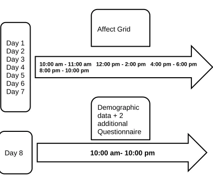
half an hour later, within the specific time slot.

Figure 1. Study Layout of ESM Study

Day 1

Day 2

Day 3

Day 4

Day 5

Day 6

Day 7

10:00 am - 11:00 am 12:00 pm - 2:00 pm 4:00 pm - 6:00 pm 8:00 pm - 10:00 pm

Day 8

10:00 am- 10:00 pm

Affect Grid

11 Participants

Twenty-six participants were recruited through convenience sampling out of the general

population, this is aligned with previous studies. Traditionally, in order to estimate how many

participants are needed, a power analysis is done. This is different in an ESM design because

reliability is achieved with many measurements instead of many respondents. In this study, it was

chosen to have at least 25 participants because Van Berkel and his colleagues (2018) provided in

their research article that a median number of 19 participants provides representative insight into

experiences or feelings. In ESM Studies the sample size is most of the time small because ESM

studies tend to employ analyses with substantially larger power such as linear mixed models that

adequately deal with the nested structure of the data. Participants were approached through various

social media channels or through family, friends or other acquaintances.

The inclusion criteria were (1) the participants had to be over 18 years old, (2) they had to

be studying at a university or university of applied science and/or be employed, (3) they had to

have an iOS or Android-capable smartphone, (4) they were able to properly understand and

comprehend the English language. Participants were excluded from this study by the following

exclusion criteria; (1) did not agree with the informed consent, or (2) did fill in the affect grid less

than 13 times.

Materials

TiiM (The incredible intervention machine)

In order to take part in the study, participants had to download the TIM application. This is an

application that was developed by researchers from the University of Twente and functions as a

means of conducting research online. Participants received a registration link with which they were

able to register for the study and create an account in TiiM. With the start of the study, participants

received notifications regarding the questions they needed to fill out each day (Appendix 3).

Affect Grid

The Affect Grid is a single item scale that was developed to measure a person's emotional state. It

is based on the circumplex model of affect, in which a person’s emotional state can be mapped

onto a two-dimensional Cartesian plane where the x-axis represents a pleasure-displeasure

12

version of the affect grid had the form of a 9x9 grid and participants had to mark an X in the square,

to indicate how he or she is feeling at the moment. Since the original affect grid was a pen and

paper version, it resulted in participants only making use of the space within the square, not being

aware that they also could mark their X everywhere within the grid. Thus, the outcome tended to

be skewed (Russel, Weiß, & Mendelsohn, 1989). Over time, the Affect Grid and the wordings of

the x and y-axis were altered. Nowadays, the most common wordings are a pleasure for the x-axis

and energy for the y-axis (Russel, Weiß & Mendelsohn, 1989). The Affect Grid was chosen due to

the fact that it is quickly filled out and consequently can be used rapidly and repeatedly. In this

study, the Affect Grid is used to measure state feelings and moods of participants throughout the

study. The original Affect Grid was altered in order to be used in this study, in a digital form and

also to undermine the probability of getting skewed data. Participants in this study could mark their

emotional state with a dot, anywhere within the Affect Grid, which they moved with the

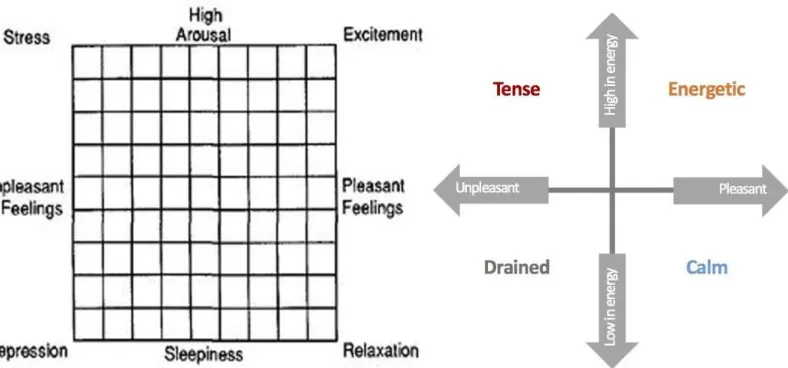
touchscreen of their mobile phone. In figure 2, the original version as well as the altered version,

used in this study, are depicted.

Figure 2. Original Affect Grid (left) and altered Version of the Affect Grid used in this study

(right).

Positive and Negative Affect Scale (PANAS)

The Positive and Negative Affect Scale (PANAS) was developed to measure mood or emotion

13

PANAS is a self-report scale and consists of 20 items, with 10 measuring positive affect (PA) and

10 measurings negative affect (NA). Items are rated on a five-point Likert Scale ranging from 1

being very slightly not at all to 5 being extremely. It was designed to measure affect in various

contexts such as; the present day, past day, week, or year, or in general (Watson, Clark, & Tellegen, 1988). Since for this study the PANAS is used for a trait measure, the questions were asked with the intonation on "the past week". The final score is measured by taking the sum of

the 10 terms on the positive scale and the sum of the 10 terms on the negative scale. Scores on

each scale can range between 10 to 50 with higher scores on the PA scale representing higher

levels of positive affect and vice versa for the NA scale. Values assigned are positive for answers

on the positive scale and negative for answers on the negative scale (Watson, Clark, & Tellegen, 1988). In a sample of international students, with 9 females and 9 males (the average age was 28) Thompson (2007) found high reliability for the NA scale with Cronbach’s alpha being 0.82 and

for the PA scale, Cronbach’s alpha being 0.85. The PANAS has a strong convergent validity with

such measures as general distress, depression and state anxiety (Thompson, 2007). In this study,

the Positive affect scale of the PANAS also showed high reliability with Cronbach’s alpha being

0.74. Likewise, the negative affect scale has shown high reliability with a Cronbach’s alpha of

0.87.

Toronto Alexithymia Scale (TAS-20)

Besides the PANAS, the Toronto Alexithymia Scale (TAS-20) was used. It was developed to

measure alexithymia and is one of the most commonly used tests for that. The TAS-20 is a

self-report scale and consists of 20 items with three different subscales. The Items are rated by using a

five-point Likert scale whereby 1 is "strongly disagree" and 5 is "strongly agree". In order to get a

total alexithymia sore, responses are summed over all 20 items. For the subscales, each subscale

factor is the sum of the responses to that subscale. The TAS-20 uses cutoff scoring which means

that a score of equal to or less than 51 means non-alexithymia, a score equal or greater than 61

means alexithymia and scores between 52 to 60 mean possible alexithymia (Bagby, Parker, &

Taylor, 1994).

In a sample of 389 male and 576 female students from a Canadian university with 21.8

(SD=5.6) being the mean age, Bagby, Parker, and Taylor (1994) found high reliability, with Cronbach’s alpha being 0.81. In this study, the TAS20 has shown high reliability with Cronbach’s

14 Pilot Study

In order to check the usability of the application and the understanding of the questions, before the

final study, a pilot was conducted. Two people were asked to take part in the pilot test which took

place for three days. Also, both researchers and the supervisor of this bachelor's project took part.

Both participants understood the questions asked but for the use of the application it was decided

to provide future participants with a handout, in which it was explained step by step how to

download the application and set up an account. Likewise, for the final study, instructions were

added in the application on how to deal with the tools such as the Affect Grid and the Likert scales.

Procedure

This study was approved by the BMS Ethics Committee of the University of Twente (#190452).

Participants were recruited via convenience sampling through various Social Media channels. First

participants were informed about the purpose of the study, confidentiality regarding their data, and

agreed on the terms and conditions of the study (Appendix 1). A handout was offered, in which it

was explained which steps have to be done in order to participate and how the application TIIM

application works (Appendix 2). All questionnaires and scales mentioned above were merged into

one “intervention” in TiiM. In the first seven days starting from a Tuesday morning at 10:00 am,

the participants were asked to fill out the Affect Grid and two additional questions regarding

anxiety and depression four times a day, in a specific time slot, determined by the researcher. On

the last day of the study, participants had to fill out the PANAS and the TAS-20 and the HADS.

The two questions regarding anxiety and depression and the HADS were used by another

researcher. Also, they had to fill in socio-demographics including age, occupation or study, study

program, nationality, and gender. After the study, the obtained data was stored and retrieved from

TiiM.

Data analysis

The statistical program SPSS (version 25) and Microsoft Excel (16.14.1) were used for the data

analysis. Since on the last day of the study the application did not work for some participants, it

was required to make use of Qualtrics and send the baseline questionnaires PANAS, TAS20, and

questions about the demographics to five participants who were not able to fill out these

questionnaires via TiiM. First of all, the data from TiiM and from Qualtrics were transformed into

15

included in the analysis, due to the fact that all completed the questionnaire in TiiM frequently, (all

participants completed the questionnaires at least 13 times). In order to get information about the

demographic variables such as age, gender, nationality and student and/or job, descriptive statistics

such as means, standard deviations, frequencies, were used. For the reliability of the questionnaires,

a reliability analysis was conducted, to get the score of Cronbach’s alpha. For PANAS and TAS20,

the sum scores of participants and means and standard deviations were calculated.

In order to make use of Linear Mixed Modeling (LMM), the data set was changed into a

long format. Linear Mixed Modeling was used to analyze the data of this study because it accounts

for the nested structure and missing data and therefore is especially useful for ESM data. Thus, a

series of LMM analyses with an autoregressive covariance structure was conducted to analyze the

hierarchical structure of the repeated measurements per participants and/or time. All mean values

gathered by LMM take missing data into account and are as a consequence estimated and referred

to as marginal means. In each LMM analysis, the subjects were the participants, the measuring

point was repeated and the repeated covariance type was AR(1). The dependent variable was either

x (pleasure) or y (energy), of the Affect Grid. The measuring point was set as a fixed factor and

was added to the model. This was done in order to get the estimated marginal means for each

measurement point to be able to compare the data over the different time points and to see how

participants feelings changed or varied throughout the study. In order to get information about each

participant, the fixed factor participant was added to the model. In this way estimated marginal

means for each participant were estimated, to be able to compare participants. The output of the

analysis mentioned above provided a mean estimation of the dependent variables pleasure and

energy, of the affect grid. Next, PA and NA of the PANAS and the grouped TAS20 scores were

added as a fixed factor into a series of separate LMM analyses, in order to get an estimation of

F-values. In the same analysis, either PA or NA affect of the PANAS were added as covariates in

order to estimate their correlation to the dependent variables pleasure or energy of the affect grid.

To be able to estimate the correlation of the grouped TAS20 scores to the dependent variables was

added as a covariate but measurement point was not added as a fixed factor because otherwise,

SPSS did not provide an output. To be able to compare the estimated means of the variables and to

create graphs to visualize how the various variables were related to each other, Excel was used.

Graphs were created for measurement points over time and between participants.

In order to confirm the outcome of the LMM analyses, a series of post-hoc bivariate

16

participant's overall mean state of pleasure or energy on the different time points of measurement.

Likewise, a post-hoc bivariate correlation analysis was used to examine the relationship between

the overall mean state of pleasure and energy of participants, with the overall positive and negative

affect of the PANAS of the participants.

Based on the outcomes of the TAS20 questionnaire, participants were divided into two

groups. Participants without alexithymia (0) and Participants with alexithymia (1). This

questionnaire is used to see in what degree participants are able to identify their emotions and

whether people who have no signs of alexithymia have a different level of state emotions

throughout the day. It was decided that participants with a sum score of 55 or higher, have

alexithymia and participants below that score do not. It was decided because 55 is approximately

the middle score. Thus, 15 participants showed no signs of alexithymia whereas 11 participants

did. This allows evaluating differences between individuals showing signs or no signs of

alexithymia. Furthermore, these groups' pleasure and energy levels were analyzed with bivariate

correlation analysis. A bivariate correlation for the groups' pleasure/energy and their positive or

negative affect was as well analyzed, to get information regarding their trait and state measures,

and to check whether the participants who have alexithymia differ in that aspect as well from the

participants who do not. The effect sizes of the analyses were interpreted on the basis of Cohen's

conventions (1988), in which a coefficient of .10 is considered as a weak correlation, a coefficient

of.30 a moderate and a coefficient of 0.50 a strong correlation.

For the purpose of getting in-depth information about participants with extreme scores, 2

individuals were picked. Their scores of pleasure and energy of the affect grid were visualized in

graphs, likewise, their affect grid was replicated.

Results

Demographic variables

In total, there were 26 participants who downloaded the TiiM application and completed the study.

The mean age of the participants was 23.7 (SD= 3.71), with 15 being female and 11 male. There

were 16 students, of which 11 had a student job, the rest of the sample consisted of people who

have a full-time occupation (Table 1). All 26 participants were included in the analysis. The

17

Table 1. Demographic variables of participants.

Item Category Frequency %

Gender Male

Female

11

15

42.3

57.7 Nationality German

Dutch Other (British) 23 2 1 88.4 7.7 3.8

Job Yes

No

21

5

80.8

19.2

Student Yes

No 16 10 61.5 38.5 Descriptive statistics

State pleasure and energy over the time of 7 days

By running a Linear mixed model analysis, the participants' pleasure and energy throughout the

study were analyzed. The estimated marginal means of all 28 measuring points of all participants

can be seen in Figure 2. The average amount of pleasure was estimated being 19.50 (SD=9.30),

over the 28 measuring points. The average level of energy was -7.16 (SD=10.1). Overall there was

a wide variation in mean scores across the measurement points. Participants scored the highest

pleasure, with the mean being 33.66 (SD=10.30), on the 17th measurement, which equals to

Saturday morning (Time of measurement 8:00 - 10:00 a.m.). Their lowest pleasure level was on

the 21st measurement with a mean of 2.85 (11.86), this measurement was taken Sunday morning

18

measurement with a mean of 12.2 (SD=9.86), which was taken Wednesday (12:00 - 2:00 p.m.). On

the contrary, their lowest energy was on the 20th measurement, with a mean of -26.34 (SD=10.13),

which equals to Saturday evening (8:00 - 10:00 p.m.) (Figure 2). Having a look at the graph,

suggested that higher pleasure levels do not indicate higher energy levels.

Figure 2. Estimated marginal means of pleasure and energy for all 28 measuring points, of all

participants

State Pleasure and Energy per Person

Analyzing the data for each participant, overall it shows that there were great variations between

participants and their feelings. Participant 9 scored the lowest overall pleasure with a mean of -

60.24 (SD=10.74) and participant 15 having the highest pleasure overall with a mean of 67.70

(SD=9.96) (Figure 3). Regarding the energy scale, it resulted in participant 6 having the highest

overall energy with a mean of 16.20 (SD=12.98) and participant 13 having the lowest overall

19

Figure 3. Estimated marginal means for pleasure and energy of all 26 participants

Comparing both the overall means of time point and participants or overall emotions in

participants showed that there was substantial variation in both. Specifically, in the pleasure scale

participants scores varied strongly. Furthermore, there was more variation and outbreaks in energy

levels throughout the weekend than on weekdays, which can be seen in Figures 2 and 3.

Additionally, the participants had higher levels of pleasure than energy throughout the week

compared to weekends.

PANAS

On the eight day of the study, participants were asked to fill out questionnaires such as the PANAS

and the TAS20. The PANAS is used, in order to check how their trait affect is associated with their

state affect. The participants' overall positive affect was 33.10 (SD=5.60) and the overall negative

affect was 25.41 (SD=11.79). Meaning that the participants all together perceived more positive

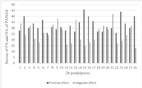
than negative affect. Overall, in Figure 6, it can be seen that in most participants the levels of

positive affect are much higher than the negative affect. But for example, in 9 participants, the

scores of negative affect are higher than the positive affect. Participant 9, also as can be seen in

figure 4, had very low pleasure levels, this suggests that state feelings, do reflect themselves in the

20

the lowest was 26, for participant 7. The highest score for negative affect 42, for participant 21 and

the lowest score was a 13, for 26.

Figure 6. Sum scores of the positive and negative affect of the PANAS for all 26 participants

TAS20

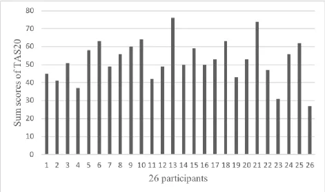
The participants average of the scores of the TAS20 was 52.27 (SD=11.70). Meaning overall

participants possible show signs of alexithymia. From the 26 participants, 11 show no signs of

alexithymia, 6 showed signs of it and 9 showed possible signs of alexithymia (Figure 7). Participant

21

Figure 7. Sum scores of TAS20 of all 26 participants

After changing the cut-off score to 55, in order to divide participants into two groups, no signs of

alexithymia and signs of alexithymia the following was found out. After this grouping, fifteen

participants had no signs of alexithymia and eleven had signs of alexithymia. In figure 8, it can be

seen that there appear to be less variation in the scores of pleasure and energy from people with

signs of alexithymia. The mean pleasure of participants with alexithymia was 15.1 (SD=31.3), their

mean energy was -1.1 (SD=17.3). The highest score of pleasure was 67.7, which belongs to

participant 7, the lowest score of pleasure was measured of participant 4, with a value of -60.2.

Participant 2, had the highest overall energy with a score of 16.2, in contrast, participant 6 had the

22

Figure 8. Estimated marginal means of pleasure (x) and energy (y) of the 11 participants with

alexithymia

As opposed to what was mentioned before, in figure 9 it can be seen that scores of pleasure and

energy of people without signs of alexithymia have huge variations. The mean pleasure of

participants without signs of alexithymia was 21.87 (SD=14.01), their mean energy was -11.98

(SD=12.87). Overall, participant 13 had the highest pleasure with a score of 40.82 and participant

11, the lowest with a score of -4.51. The highest energy was measured in participant 6, with a score

of 6.84, in contrast, participant 9 had the lowest energy with a score of -35. Considering both and

comparing figures 8 and 9, it can be seen that there are differences in levels of pleasure and energy

23

Figure 9. Estimated marginal means of pleasure (x) and energy (y) of the 15 participants without

24 Linear Mixed model

Table 2. Using different variables as covariates in the Linear mixed model

Dependent Fixed factors Covariates F-value (df1, df2) p-values

Pleasure (x) Measurement point Energy (y)

PA (PANAS)*

NA (PANAS)*

No_Yes Alexithymia*

1.060 (27, 309.0289)

14.539 (1, 126.076)

42.546 (1, 137.351)

2.068 (1, 123.210)

p=.387

p=.000

p=.000

p=.153

Energy (y) Measurement point PA (PANAS)*

NA (PANAS)*

No_Yes Alexithymia*

0.000 (1, 174.080)

0.105 (1, 175.426)

5.976 (1, 178.873)

p=.978

p= .746

p=.015

*Measurement point was not added as a fixed factor to the model otherwise the model would not provide an output

State and Trait Measures

By running a bivariate correlation analysis, Pearson's correlation revealed a weak non-significant

negative correlation between state pleasure and state energy throughout the 28 measuring points

(r= -0.128, p =.516). This implies that pleasure and energy levels did not correlate with each

other over the 28 measuring points. Another Pearson’s correlation revealed a strong significant

negative correlation for the trait positive affect and trait negative affect of the PANAS (r=-.520,

n=26, p=.007). This indicates that when Positive affect increases in a person, then negative affect

decreases (Appendix 5).

Association between dependent and independent variables

By adding trait positive affect as a covariate, in the LMM analysis, it showed that positive

affect did significantly covariate with state pleasure F (1, 126.076) =14.539, p=.000. The

post-hoc bivariate correlation analysis confirmed the effect because a moderately significant positive

25

their trait positive affect was found. Indicating that when participants' pleasure increased, their

overall positive affect increased as well. Trait negative affect was added to the LMM analysis as

a covariate of state pleasure of participants, it revealed a significant main effect F (1, 137.351)

=42.546, p=.000. Afterwards a post-hoc bivariate analysis was conducted. A strong significant

negative correlation was found between the estimated mean pleasure of participants and the

negative affect of participants (r=-.664, n=26, p=.000). This suggests that when levels of pleasure

of participants increased, their overall negative affect tended to decrease.

In separate LMM analysis, each positive and negative affect were added as covariates, but

both did not have a significant effect on energy levels (Table 2). A post-hoc analysis for the level

of energy and positive affect of persons, there was a weak non-significant positive correlation

found (r=.048, n=26, p=.814). For the level of energy and negative affect, there was also a weak

non-significant positive correlation found (r=.057, n=26, p=.781). Both suggesting that state energy

does not influence the individual's overall positive or negative affect (Appendix 5).

Association of TAS20 scores with the Affect Grid and PANAS

Adding the overall score of the TAS20 of the participants as a covariate to the state pleasure

of participants, in the LMM, resulted in a strong significant main effect F (1, 123.210.) =2.068,

p=.153. As well adding the overall TAS20 score as a covariate to state energy of participants

resulted in a strong significant main effect F(1,178.873)=5.976,p=.015. Indicating that TAS20

scores correlate with both pleasure and energy scores, thus when TAS20 scores are higher, both

state pleasure and energy are higher as well.

Two bivariate correlation analyses were conducted for the participants who showed signs

of alexithymia and the participants who did not show signs of it. The bivariate correlation analysis

of the pleasure and energy scores of the 11 participants with signs of alexithymia revealed a strong

significant positive correlation (r=.643, n=11, p=.034). It indicated that when pleasure levels

increased, energy levels of participants with signs of alexithymia increased as well. On the

contrary, after conducting a bivariate correlation analysis for the scores of pleasure and energy of

the 15 participants with no signs of alexithymia revealed a moderate non-significant negative

correlation (r=-.321, n=15, p=.243). Suggesting that, levels of pleasure and energy did not increase

or decreased, when one of them increased or decreased, in participants without signs of alexithymia

26

Lastly, to check whether there are different associations of scores of the affect grid and the

PANAS of participants with and without signs of alexithymia several bivariate correlation analyses

were conducted. For PA and pleasure levels of participants with alexithymia, it revealed a strong

significant positive correlation (r=.633, n=11, p=.037). Implying that when pleasure levels

increased, positive affect increased as well, similar to what was found with the bivariate correlation

analysis of all 26 participants levels of pleasure and PA. For the participant's levels of pleasure and

their negative affect, the analysis revealed a strong negative significant correlation as well (r=-.672,

n=11, p=.024). This is likewise similar to what was found when doing the analysis with all 26

participants. For participants with signs of alexithymia with regard to their overall PA and their

energy levels, the Pearson correlation indicated a moderate positive non-significant correlation

(r=.357, n=11, p=.281). This suggests that when their energy levels increased, their overall PA did

not increase. On the contrary, with regards to their overall NA and their energy levels, it indicated

a strong negative significant correlation (r=-.544, n=11, p=.084). Indicating that when levels of

energy increased, their NA decreased (Appendix 6).

For participants without signs of alexithymia, there was only one significant finding.

Correlating their overall NA with their pleasure levels revealed a strong negative significant

correlation (r=-.745, n=15, p=.0013). Suggesting that when their pleasure levels increased, their

NA decreased. These findings, implicate that participants with alexithymia and participants without

alexithymia do differ in how they perceive their feelings (Appendix 6).

Individual analysis

Having a closer look at participant 9, resulted in the findings of figure 4. It can be seen that

throughout the study, the participants' levels of pleasure are very low most of the time, on the

contrary, the energy levels of the participants vary a lot throughout the study. Considering the affect

grid, the participant most of the time feels drained, with a few times feeling calm. This can also be

27

Figure 4. Scores of the Affect Grid of Participant 9 throughout the study

In figure 5, the scores of pleasure and energy of participant 15 have been put into a graph. It can

be seen that the pleasure levels are mostly stable and high throughout the study. Opposed to that,

are the energy levels. They vary a lot throughout the study. Especially in the measuring points 9 to

11, which equals to Thursday noon, afternoon and evening. Here it can be seen that the participants

experience the lowest levels of energy on Wednesday afternoon but in the evening, the energy is

very high with a score of 99. The same results can be seen for the measuring points 12 through15,

which equal to Friday morning to evening. In the mornings, the level of energy is the lowest, with

28

Figure 5. Scores of Pleasure and Energy of Participant 15 throughout the study

In Figure 6, the scores of the affect grid of participant 15 are displayed. Here it can be seen that the

participant felt tense most of the time but a few times, the participant felt energetic. This is similar

to what can be seen in Figure 6, where it is displayed that the participants' levels of energy vary

29

Figure 6. Scores of Affect Grid of Participant 15.

Discussion

This study's objective was to gain an impression of the variety of momentary emotional states and

how they differ throughout the day and within persons themselves. One of the main findings of this

study was that when comparing the trait feelings and the state feelings of participants, there are

indeed variations. Feelings as already mentioned in the introduction, are not stable, but change,

considerable also within a day. This study indicated that experience sampling appears to be a

suitable method to catch the dynamic of feelings because it provided information about the

variations of feelings, participants had throughout the study. It showed that state feelings and trait

feelings do correlate but not too strong, indicating that state measures do give insight into the

dynamics of feelings in a way that trait measures cannot. Thus, ESM in this study was a valid way

of measuring feelings.

Another result showed that, in this sample, pleasure and energy levels differ a lot as well,

meaning that they are not associated with each other. A person can feel energized without having

pleasure or vice versa. Accordingly, this confirms the independence of the two axes in the Affect

30

are not correlated, this again confirms the independence of the different axis of the affect grid.

Nevertheless, it has to be mentioned that a person perceives higher levels of energy/pleasure when

she or he already feels higher levels of pleasure/energy (Russel, 1980). Based on this, it can be

concluded that an effective way of measuring state emotions are scales which treat emotions as

dimensions and not as discrete entities. This is in accordance with Russel (2009), who found out

that it is more effective to measure emotions in a dimensional way since in dynamic models of

emotions, emotions are not treated as discrete entities but rather are dimensional.

Overall, the participants scored higher on pleasure than energy. This is in accordance with

the study of Zelenski and Larsen (2000), in which they found out that their participants overall

perceived much more positive emotions than negative ones. Logically, they perceived more

pleasure on Saturday morning. This can be assumed since the sample consisted of people with a

job or students, meaning that they had free time and were able to choose which activities to do.

Likewise, great variations among participants were found. this was expected due to the fact that in

a sample derived from a normal population, people differ in their feelings. Again, this is similar to

what Zelenski and Larsen (2000) found out when comparing undergraduate students with each

other. An interesting finding was when looking at the participant which scored the lowest overall

pleasure over the duration of the study, the participant's levels of pleasure throughout the study

were very low and did not vary much. In contrast to that, the energy levels varied a great amount.

Also, the trait negative affect was lower than his/her positive affect, implicating that state

levels indeed give information about the trait behavior of emotions of the person. This is in

concordance to what Watson and Tellgen (1985) found out. The PANAS is orthogonally rotated to

the pleasure-arousal dimensions, indicating that pleasure measures do provide the same

information as positive affect measures. This again, indicates that an ESM study is able to capture

detailed information about a person's emotional life, which trait-like tests such as the PANAS,

which are applied only on one-time point, cannot capture or account for. Another finding which

supports this indication was illustrated by the case study of pleasure and energy levels throughout

the study of participant 15. The pleasure levels were high and stable, but the energy level varied

much. When looking at specific days and time periods of dates, it showed that the participant

experienced lower energy levels in the morning and much higher energy levels in the evenings.

This detailed information cannot be provided with traditional ways of studying feelings and moods,

31

result is similar to what Klerman (1988) had found, people perceive higher energy levels in the evenings and perceive depressive-like symptoms in the mornings.

Versluis and her colleagues (2018) did an ESM study, in which they checked whether

emotional awareness varies over time or is stable. Their results have shown that indeed, emotional

awareness varies over time. Thus, this provides evidence that emotions are not stable rather they

vary. This study found similar results in that respect as well. The results have shown that emotions

vary over time. Compared to the PANAS, which is only applied once and retrospectively, the ESM

with the use of the affect grid provides evidence that feelings vary and change, even within days.

Both the Versluis study (2018) and this study did not determine what these variations are due to,

meaning that they did not measure the context, thus there is no clear explanation for the variations.

Another aspect they are similar is that the real-life variations in emotions meaningfully capture the

variability within subjects in the complexity of emotional experience over time.

Comparing the findings of this study, to one of the first studies which studied trait and state

emotions while using ESM, showed interesting findings (Zelenski & Larsen, 2000). First of all,

similar to what Zelenski and Larsen (2000) have found, is that feelings do vary over time and there

are a variety of feelings, people experience throughout the day. Their results with regards to

positive and negative emotions were similar, indicating that in a non-clinical population, positive

emotions are much more prominent. This study, similar to what Zelenski and Larsen (2000) found

out, supported the assumption of Watson and Tellegen (1985) that trait emotions are perceived in

a dimension of positive and negative affect. Since this study did not check for the intensity of

feelings, no comparison with regards to the results of Zelenski & Larsen can be made. Likewise,

no comparison of the amount of blend within the categories of negative and positive emotions can

be made. Surprisingly, their results concluded that state emotions conform more to discrete

emotions model rather than dimensional ones, in contrast, trait emotions did conform to the

dimensional model. The current study cannot come to such a conclusion since for both state and

trait measurements, dimensional models of emotions were used.

Participants on average had a higher trait positive affect than negative affect, this implies

that participants generally have more positive emotions than negative ones. Again, this is in

concordance to what Zelenski & Larsen (2000) found out when comparing state and trait

feelings. Besides this study confirms what Zelenski & Larsen (2000) found out, negative

emotions were rated lower than positive ones. Comparing the state levels of pleasure of people

32

account for 16% variance of positive affect, indicating that there is a difference and thus

measuring state is important. They correlate with each other, indicating that the more pleasure

they perceived throughout the week of measuring, the higher their trait score of positive affect

was. This is in accordance with what was expected because the PANAS asks about the emotions

the participants experienced in the last week. Thus, higher scores of pleasure throughout the week

indicate higher positive affect scores. Also comparing the state levels of pleasure of people with

their trait negative affect, provided an interesting finding. The more pleasure they perceived

throughout the week, the lesser their negative affect score was.

Surprisingly, state pleasure did account for 44% of the variance for negative affect, this

indicates that state feelings are associated with trait feelings but catch dynamics in feelings which

trait measurement of feelings cannot. As already mentioned above, since the PANAS asks for

emotions participants experienced last week, this result is aligned with the one mentioned

beforehand. Meaning that higher scores of pleasure indicate lesser negative affect in persons.

Once more, this is in accordance with the Zelenski and Larsen study (2000), the more positive

emotions participants perceived, the lesser were the negative emotions they perceived. On the

contrary, when comparing the state energy of people with either the trait positive or negative

affect, there were no associations. The state energy of people did not affect their trait positive

affect, this means that regardless of how high or low their energy was in the week, their positive

affect score did not change. This is also an interesting outcome since energy is one of the axes of

the affect grid which measures mood. This is aligned with Russel, Weiss, & Mendelsohn (1989)

had found out when they studied the relationship between PA and NA affect of the PANAS with

pleasure-arousal of the Affect grid. Neither PA nor NA were correlated with arousal (or energy in

this case), indicating that the PANAS does not measure the same thing as arousal (energy), when

orthogonally rotated, although it measures pleasure, when rotated.

With regards to the TAS20, it has been shown that this sample, in general, using the

validated cut-off scores, shows no signs or some signs of alexithymia, which means most

participants do not have difficulties to identify or describe their feelings. After categorizing the

sample into two different groups with different cutoff scores, one having no signs of alexithymia

and, one having signs of alexithymia, almost half of the sample does show signs of alexithymia.

Findings have shown that participants with signs of alexithymia do not differ too much in their

pleasure and energy levels. This implicated that in this sample, people with signs of alexithymia

33

energy. As hypothesized, on the contrary participants without signs of alexithymia showed a lot of

variation, suggesting that these participants had no difficulties differentiating or identifying their

emotions throughout the week. Furthermore, it has been revealed that the higher the alexithymia

scores, the lower the pleasure and energy levels of the participants have been. This is in accordance

with the literature, stating that people who show signs of alexithymia have difficulties

differentiating between various emotions (Taylor, Ryan, & Bagby, 1985).

Comparing the scores of pleasure and energy of participants with and without signs of

alexithymia, showed that overall, participants with signs of alexithymia score lower in both

pleasure and energy. Previous studies about alexithymia and mood disorders such as the one from

Ebner-Priemer, Eid, Kleindienst, Stabenow, and Trull (2009), had found out that people with alexithymia show more negative emotions than positive ones. This is due to the fact that people

who show signs of alexithymia are much more prone to psychopathological symptoms such as

depressive episodes and mood swings (Ebner-Priemer, Eid, Kleindienst, Stabenow, & Trull 2009). Interestingly, when participants with alexithymia levels of pleasure increased, their energy levels

increased as well, indicating that they do not differentiate between those dimensions, again

confirming what Taylor, Ryan, and Bagby (1985) had found out. In contrast to that, it has been

revealed that increases in the level of pleasure do not indicate increased levels of energy for

participants without signs of alexithymia. Indicating that participants without signs of alexithymia

differentiate between the different dimensions of the affect grid.

Interpreting the results of the study, a few limitations have become prominent. First of all,

the study was done via an application that showed to have some malfunctions. Participants

complained that the app did occasionally not save their answers, or even when choosing an answer,

the application still indicated that no answer was chosen which raise difficulties continuing with

the surveys. Thus, participants sometimes needed much more time to fill out the questionnaires,

which left them annoyed and frustrated. This could have influenced their levels of pleasure and

energy throughout the study and hence altering the results. Another limitation is the fact that this

study was compiled with another researcher, which made use of other questionnaires for the ESM

and for the trait questionnaires. The fellow researcher studies depression and anxiety, therefore

maybe the participants were biased with negative wordings before filling out the Affect Grid,

meaning an ordering effect could have been possible. This could have led to declines in pleasure

34

question regarding depression, the question regarding anxiety were organized was randomized

throughout the day.

Nonetheless, a major strength of this study was the use of Linear Mixed models, which

accounted for the missing data and since it was much data that was acquired, the missing data was

no burden. A linear mixed model is a powerful analysis but when using bivariate correlation

analysis as a post-hoc analysis, the study was underpowered. Another major advantage of this study

is the use of ESM, in this way current feelings and mood states of the participants in their natural

environment have been acquired. This gives in-depth inside about the emotional state's participants

perceives not just throughout the week but also throughout the day. In line with this advantage is

the fact that ESM is a rather new approach to studying emotions and therefore has not been often

used. ESM makes it possible to study emotional states of participants throughout the day in their

natural life. Particularly in the way this study is designed, it has not been used yet. Although there

are already a few studies that make use of ESM in order to get in-depth information about emotional

states, none of them validates them with a trait questionnaire in order to see whether ESM data is

valid. Likewise, the use of the TAS20 to screen for persons with signs of alexithymia has not been

acknowledged even though one study uses the emotional awareness scale, which has a subscale for

alexithymia. The fact that this study, made use of the affect grid, which can be filled out in a few

seconds, made it more bearable to conduct a longitudinal study and thus made it more applicable

for the use with students or full-time employees. Another aspect to consider is the fact that this

study did not ask in particular what the individuals did during the time slots where they had to fill

out the questionnaires. Hence, no detailed information can be given, why in specific time points,

participants scored high or low in pleasure and energy dimensions of the affect grid.

With regard to this study, it has become more certain, that feelings and moods vary a lot,

not just within a person but also through different time points. The use of ESM provides a good

and valid way to assess state feelings as well it enriches our understanding of emotions. Likewise,

it has become evident that Alexithymia does not only appears in clinical but also in non-clinical

populations. Alexithymia needs to get further acknowledged in studies conducting research about

feelings or emotions in general. Concluding this, the study provides evidence for the fact that state

feelings differ from trait feelings and that there are variations within feelings and moods, not just

within populations but within persons and days as well.

In order to raise awareness of this aspect of emotions and to go from differences within