University of Warwick institutional repository: http://go.warwick.ac.uk/wrap
This paper is made available online in accordance with
publisher policies. Please scroll down to view the document
itself. Please refer to the repository record for this item and our
policy information available from the repository home page for
further information.
To see the final version of this paper please visit the publisher’s website.
Access to the published version may require a subscription.
Author(s): David Hobson and Anthony Neuberger
Article Title: Robust Bounds for Forward Start Options
Year of publication: Not yet published
Link to published version:
Not yet published
Robust Bounds for Forward Start Options
David Hobson
†Anthony Neuberger
‡First version: October 9, 2008,
This version: December 16, 2009
Abstract
We consider the problem of finding a model-free upper bound on the price of a forward-start straddle with payoff|FT2−FT1|. The bound depends on the
prices of vanilla call and put options with maturitiesT1 andT2, but does not
rely on any modelling assumptions concerning the dynamics of the underlying. The bound can be enforced by a super-replicating strategy involving puts, calls and a forward transaction.
We find an upper bound, and a model which is consistent withT1 and
T2 vanilla option prices for which the model-based price of the straddle is
equal to the upper bound. This proves that the bound is best possible. For lognormal marginals we show that the upper bound is at most 30% higher than the Black-Scholes price.
The problem can be recast as finding the solution to a Skorokhod embed-ding problem with non-trivial initial law so as to maximiseE|Bτ−B0|.
1
Introduction
In this article we consider the problem of pricing forward start options. More especially, if Ft is the forward price of a traded security and if T1 and T2 are
maturities withT0< T1 < T2, whereT0 is the current time, then we wish to price
a security paying |FT2−FT1|, ie a straddle with the strike set to be the prevailing
value atT1.
Our philosophy is that rather than pricing under a given (and inevitably mis-specified) model, we assume we know the call prices for maturities T1and T2, and
we use those prices to reduce the set of feasible price processes to those which are consistent with these calls under a martingale measure, and then we search over the feasible price processes to give the forward start straddle with the highest price. The pricing problem can also be expressed in a different way as a dual prob-lem where we identify the highest model price with the cheapest super-replicating hedge. The resulting price is robust in the sense that it gives a model-free no-arbitrage bound. This bound can be enforced by using calls (with maturities T1
and T2), and the forward as hedging instruments. Similar ideas have been applied
to other path-dependent options, including barrier options and the lookback option, by Hobson [11], Brown, Hobson and Rogers [4] and most recently Cox and Ob l´oj [6]. Part of the interest in the forward start straddle is that the model which attains the maximum is such that, conditional on the price atT1, the price atT2takes one
of two values (at least in the atom-free case with nice densities). As this conditional distribution places mass at two-points it can be thought of as a distribution with minimal kurtosis. In this weak sense at least, a long position in a forward start option (suitably hedged using conventional options) is akin to a short position in the kurtosis of the underlying asset.
The main result, expressed in financial language, is the following.
Theorem 1 Suppose that call prices are given for a pair of maturities T1 < T2 (for a continuum of strikes on each date) and that these prices are consistent with
no-arbitrage1. Consider the price of a forward start straddle2 on the forward price
of the asset. Then there exists a model-independent3 upper bound on the price of
this derivative; this bound can be enforced through the purchase of a portfolio of call options and a single forward transaction. Moreover, there is a model which is consistent with the observed vanilla prices for which the (appropriately discounted) payoff of the forward start straddle is equal to the bound; hence the bound is a least model-free upper bound.
The model-free upper bound on the price of the forward start option with payoff
|FT2−FT1|is increasing in the final maturityT2. However, the bound on the price of
a forward start option is not necessarily decreasing in the starting maturityT1, and
there are examples where the price of a forward start straddle with payoff|FT2−FT1|
exceeds that of a vanilla at-the-money straddle with payoff |FT2−FT0|, where T0 is
the current time.
The lack of monotonicity in the starting maturity of the price of a forward start straddle is one of the surprising results of this study.
As noted by Breeden and Litzenberger [3], knowledge of European call option prices (for the continuum of strikes) is equivalent to knowledge of the marginal distributions of the price process under a risk-neutral measure. Hence we will assume that we know the laws of X ∼FT1 andY ∼FT2 and that they are given
1We say that a set of traded securities is consistent with no arbitrage if there is no portfolio of
traded instruments (which in our case are the puts and calls with maturitiesT1andT2, and the riskless bond) which can be combined with a simple semi-static hedging strategy in the forward (buy and hold over (0, T1] or (0, T2] or (T1, T2]) such that the initial cost is zero but the final payoff is non-negative almost surely, and positive with positive probability. The fact that a butterfly spread has a non-negative payoff means that it must have a non-negative price, else there is an arbitrage. Hence option prices for a fixed maturity must be convex in the strike. Similarly, option prices must be increasing in maturity. For further discussion, see, for example, Davis and Hobson [7].
2We generally work with the straddle, but from the identity|y−x|= 2(y−x)+−(y−x) it is clear that the results can be reformulated in terms of puts or calls.
3If the call prices with maturitiesT
byµand ν respectively. By the martingale property we haveE[Y|X] =X so that
µ and ν have the same mean. Typically, we will use a shift of coordinate system and assume the mean to be zero. However, in the sections on the financial context where the marginals are derived from positive prices and the associated measures lie on R+, this is not appropriate and we will assume that the measures have equal but positive means.
DefineH(µ, ν) := supE|Y−X|, where the supremum is taken over pairs of ran-dom variables (X, Y) with the appropriate marginals, and satisfying the martingale conditionE[Y|X] =X. The problem of calculatingHcan be recast as a Skorokhod embedding problem for Brownian motion B (Skorokhod [17], see also Ob l´oj [14] for a thorough survey). The Skorokhod embedding problem (SEP) for Brownian motion null at zero is, given a centred probability measure ν, to find a uniformly integrable4 stopping timeτ such that B
τ ∼ν. Our problem is a variant on this
in the sense that instead of B0 ≡ 0 we have B0 ∼ µ. The problem becomes to
find the solution of a SEP with given initial and terminal laws with the additional optimality property that E[|Bτ−B0|] is maximised. Since, in general, there is no
unique solution to the SEP, adding an optimality criterion has proved to be a useful way of characterising solutions with particular properties (eg Az´ema and Yor [1], Perkins [15], Jacka [13] and Vallois [18], and, for the problem with non-trivial initial law, Hobson and Pedersen [12]). The connection between the forward start option and the SEP is made precise by identifying X with FT1 and B0, Y withFT2 and
Bτ, and noting that the martingale property of the forward price means that it is
a time-change of Brownian motion.
The first and most immediate question is to determine when the problem is feasible, in the sense that given centred probability measures µand ν, when does there exist a martingale with initial distribution µ and terminal distribution ν. By an application of Jensen’s inequality it can be seen that a necessary condition for such a martingale to exist is that µ ν in the sense of convex order — by construction of solutions of the SEP this can also be seen to be sufficient.
We want to studyH in the feasible caseµν.
Proposition 2 Supposeµ, ν, χ are centred probability measures, and thatµ≺ν ≺
χ in the sense of convex order. Then H(µ, ν) ≤ H(µ, χ). However, it is not
necessarily the case that H(µ, χ)≥H(ν, χ).
This counter-intuitive result (see Lemma 4 and Example 5 below) is indicative of some of the subtleties of the problem. Nonetheless it turns out that optimal solutions always exist, and they always have a particular simple form whereby conditional on X, Y takes one of two values (in the non-atomic case at least). In the SEP setting,τ is the first exit time ofB from an interval which depends onB0
alone.
A special case of the main theorem, Theorem 19, is the following:
Theorem 3 Supposeµ and ν are centred probability measures with bounded
sup-port, and suppose µ ν and that µ has no atoms. Then, there exist increasing
4
functions f and g with f(x)≤x≤g(x), such that if X ∼µ and if conditional on
X = x, Y ∈ {f(x), g(x)} respects the martingale properties5, then Y ∼ ν.
More-over,f, g can be chosen such that the joint law maximisesE[|Y−X|]amongst pairs
of random variables satisfying X ∼µ,Y ∼ν andE[Y|X] =X, and then
H(µ, ν) = Z
µ(dx)(g(x)−x)(x−f(x)) (g(x)−f(x)) .
One unfortunate feature of the solution is that it is non-constructive, in the sense that given general measuresµandν we are not able to give explicit formulae for f and g. (However, there are some simple examples where exact formulae can be given, and it is always possible to reverse engineer solutions by fixing µ,f and
g, subject to some consistency conditions, and deducing the appropriate law for
ν.) This is reminiscent of the situation for the barrier solution of the SEP due to Root [16].
The idea behind the proof is to write down a Lagrangian formulation of the problem, and to derive relationships between the multipliers, which ultimately give the characteristics of the optimal solution. The optimal multipliers are related to a particular convex function, but it is possible to derive a bound from any convex function. Hence, even in cases where it is difficult to determine H precisely, it is straightforward to give families of simple and concrete bounds. Inequalities derived in this fashion, see especially Example 6.2, may be of independent interest.
The remainder of the paper is structured as follows. In the next section we describe the set-up and introduce notation. In Section 3 we consider the non-monotonicity of H in the initial law. In Sections 4, 5 and we 6 we introduce the Lagrangian approach and give examples. These sections provide intuition and motivation for the later analysis. In Sections 7 and 8 we describe and prove the main result, which follows by taking limits over discrete approximations to the initial and terminal distributions. Sections 9 and 10 give further examples and financial interpretation.
2
Notation
In this article we will use three different probabilistic ups. The financial set-up involves the forward price process (Ft)0≤t≤T2. The Brownian set-up describes
a Brownian motion (Bt)t≥0, withB0 non-trivial, and Brownian stopping timesτ.
The random variable set-up consists of a pair of random variables X and Y. In each case there is an implicit probability triple and filtration (Ω,F,F,P) (which may change between the three set-ups, although we use the same symbolPin each case).
The idea is that we identifyFT1 with B0 andX and FT2 withBτ andY. The
relationship between F and B is based on the fact that any martingale (and the forward price is a martingale under a risk neutral measure) can be written as a time-change of Brownian motion. Thus we can identify price process with lawµatT1and
law ν at T2 with solutions of the Skorokhod Embedding Problem for a Brownian
5
motion started with law µand stopped to have law ν. Moreover, since the payoff of the forward-start straddle depends only on the law ofFT1 andFT2 (respectively
B0 and Bτ) we can reduce the problem further to an analysis of constructions of
pairs of random variablesX andY such thatE[Y|X] =X. Hence, when we speak about a feasible model we will typically be referring to a pair (X, Y) with X ∼µ
and Y ∼ν, but this is connected via a solution of the SEP to B0∼µandBτ ∼ν
and thence via a time-change to a financial model withFT1 ∼B0andFT2 ∼Bτ.
The fact that (Ft)t≥0 is a true martingale corresponds to τ being uniformly
integrable, and in turn to the fact that (X, Y) satisfy the martingale condition
E[Y|X] =X. Finally, all these conditions relate toµandν having the same mean. Clearly, by a shift this mean can be taken to be zero, so that µandν are centred.
LetMbe the set of feasible models, which, as discussed above, can be identified with the set of pairs of random variables with the correct marginals, and satisfying the martingale property:
M=M(µ, ν) ={(X, Y) :X ∼µ, Y ∼ν,E[Y|X] =X}.
There is a simple condition which determines whetherMis non-empty, namely that
µ ν in the sense of convex order (and we will use ≺and only in this sense), or equivalently Uµ(x) ≤ Uν(x) uniformly in x, where for a centred probability
measure χ,Uχ(x) =E[|X−x|:X ∼χ] is the potential. Note there is a one-to-one
correspondence between centred probability measures and potential functions U
with the propertiesU convex,|U| ≥xand limx→±∞U(x)− |x|= 0, see Chacon [5]. Then, providedMis non-empty we define
H(µ, ν) = sup
(X,Y)∈M(µ,ν)
E[|Y −X|],
and our primary concern is with identifying this object H.
In the exposition we will sometimes need to consider an iterated version of the problem, so for centred probability measuresµν η let
M(µ, ν, η) ={(X, Y, Z) :X ∼µ, Y ∼ν, Z ∼η,E[Y|X] =X,E[Z|Y] =Y}.
Further, for a centred measureχ, letχmbe the measure which is the law of Brownian
motion started with lawχand run until the process hits the set 2−mZ={2−mk;k∈ Z}, so χm = L(B
τ;B0 ∼ χ, τ = inf{u : Bu ∈ 2−mZ}). Equivalently, χm is the
measure with potential Um where Um ≡ U on 2−mZ and is obtained by linear
interpolation over intervals (k2−m,(k+ 1)2−m) elsewhere.
Denote byδx the point mass atx. Finally, given increasing functionsf, gwith f(x) < x < g(x), set τf,g,x to be the first time that Brownian motion leaves the
interval (f(x), g(x)) whereB0=x(we writeτf,g,x= inf{u:Bu∈/(f(x), g(x))|B0=
x}) and let ˆν(f, g, µ) =L(Bτf,g,B0;B0∼µ).
3
Monotonicity properties, and lack thereof, for
H
.
Lemma 4 (i) For µ ≺ ν, H(µ, ν) ≤ H(δ0, µ) +H(δ0, ν), and hence for centred
probability measures we have H(µ, ν)<∞.
(ii) If µ ν χ then H(µ, ν) ≤ H(µ, χ). Hence if νn ↓ ν then H(µ, ν) ≤
lim infH(µ, νn).
Proof: (i) Irrespective of the martingale condition,E[|Y −X|]≤E[|Y|] +E[|X|] =
H(δ0, µ) +H(δ0, ν). Note thatE[|Y|] =UL(Y)(0) is independent of the joint law of
X andY.
(ii) If µ≺ν ≺χ then there are constructions of random variables (X, Y, Z) such that E[Z|Y] =Y and E[Y|X] = X with the appropriate marginals. If we take a supremum over these constructions only then we find
H(µ, χ)≥ sup M(µ,ν,χ)
E[|Z−X|].
By the conditional version of Jensen’s inequalityE[|Z−X|]≥E[|Y −X|] and
sup M(µ,ν,χ)
E[|Z−X|]≥ sup M(µ,ν,χ)
E[|Y −X|] = sup M(µ,ν)
E[|Y −X|] =H(µ, ν)
Example 5 Given µ ν χ we have that H(µ, ν) ≤H(µ, χ) and it would be nice to be able to conclude also that H(µ, χ) ≥ H(ν, χ). (Then we would have that H was monotonic in its first argument, which would facilitate approximating
µ with a sequence µn.) However this is not the case, and we can have either H(µ, χ)< H(ν, χ) orH(µ, χ)> H(ν, χ).
The more usual and expected case is that H(µ, χ) > H(ν, χ). For a simple example takeν≡χ6=µ. For an example in the less expected direction takeµ=δ0,
ν to be the uniform measure on the two-point set{±1}, andχto place mass 1/2n
at±nand mass 1−1/nat the origin. ThenH(δ0, χ) = 1. However, ifY ∼ν and if
we setZ =nY with probability 1/nandZ= 0 otherwise, thenZ∼χ,E[Z|Y] =Y
andH(ν, χ)≥2(n−1)/n. (In fact it is easy to see that there is equality in this last expression.) Providedn >2 we haveH(δ0, χ)< H(ν, χ).
Recall the definition ofνm and observe thatν νm.
Lemma 6 Supposeµν. Then H(µ, ν)≤H(µ, νm)≤H(µ, µm) +H(µm, νm)≤ H(µm, νm) + 2−m
Proof: The only inequality which is not immediate is the middle one. Letσm =
inf{u ≥ 0 : Bu ∈ 2−mZ;B0 ∼ µ} and let τm be an embedding of νm based
on initial law µ. Then, necessarily, τm ≥ σm, and if θ
t(ω) is the shift operator θt(ω) = σm(ω) +t, if ˜Bt =Bθt and if ˜τ = τ
m−σm then ˜τ is an embedding of
νm for the Brownian motion ˜B started with initial law ˜B
0∼µm. By the triangle
inequality, E|Bτm −B0| ≤ E|Bτm −Bσm|+E|Bσm −B0|. ButE|Bτm −Bσm| =
E|B˜˜τ−B˜0| ≤H(µm, νm) andσmis the unique, uniformly integrable embedding of
µm for Brownian motion started with lawµ so thatE|B
4
Upper bounds and a financial interpretation
Suppose we can findα,β andγsuch that for allxandywe haveL(x, y)≤0 where
L(x, y) =|y−x| −α(x)−β(y)−γ(x)(x−y). (1)
If so then for all elements of the sample space,
|Y −X| ≤α(X) +β(Y) +γ(X)(X−Y),
and, taking expectations and using the martingale property,
H(µ, ν)≤
Z
α(x)µ(dx) + Z
β(y)ν(dy).
The following simple example is a first illustration of the method and gives a sample result. For k >0, 0≤k(|b| −1/k)2/2 and so, withb =Y −X, and using
(Y −X)2=Y2−X2+ 2X(X−Y), we have
|Y −X| ≤k2 Y2−X2+ 2X(X−Y) + 1
2k.
Hence, (recall we are assumingE[Y|X] =X) for anyk,E|Y−X| ≤(kA2/2) + 1/2k
whereA2=E[Y2]−E[X2] =E[(Y−X)2]. Minimising overkwe findk=A−1, and
so
E|Y −X| ≤A≡pE[Y2]−E[X2].
We can get this result directly (ie without writing down the pathwise inequality) just from Jensen’s inequality:
E|Y −X| ≤(E[(Y −X)2])1/2=A
but one advantage of the method based on inequalities of the form L(x, y)≤0 is that the various terms can be meaningfully identified in the financial context as static hedging portfolios. Thus α(X) is a portfolio of options with maturity T1,
β(Y) is a portfolio of options with maturityT2, andγ(X)(X−Y) is the gains from
trade on the forward market from a strategy of going shortγ(X) forwards over the period [T1, T2]. It is also possible to identify when the bound is tight. In this case
we must have|Y −X|= 1/k=A, so thatY =X±1/k.
Lemma 7 Consider the problem of hedging a forward-start straddle on the forward
price Ft with payoff |FT1 −FT2|. Suppose that α, β and γ are such that (1) holds,
and thatαandβ are twice differentiable6. Then there is a super-replicating strategy
involving puts and calls onFtwhich costsRα(x)µ(dx) +R β(y)ν(dy)whereµis the
law of FT1 andν is the law ofFT2.
Proof: By the arguments of Breeden and Litzenberger [3] it is possible to recreate a (sufficiently regular) payoff of Γ(FT) as a portfolio of put options with strikeK:
Γ(FT) = Γ(0) +FTΓ′(0) +
Z ∞
0
Γ′′(k)(k−FT)+dk.
6
We need to give a suitable interpretation toα′′andβ′′, so that a weaker sufficient condition
Note that (k−FT)+ is the payoff of a put with strikekand maturityT.
Consider the strategy of purchasing a portfolio of puts with maturityT1 which
recreates a payoffα(FT1) and a portfolio of puts with maturityT2 which recreates
a payoffβ(FT2).
In addition, if atT1 the priceFT1 =x, go short γ(x) units of the forward over
the period [T1, T2].
The final value of this portfolio isα(FT1) +β(FT2) +γ(FT1)(FT1 −FT2) which
super-replicates |FT2−FT1|. Since the forward transaction is costless, the cost of
the super-replicating strategy is as claimed.
Remark 8 (i) We should emphasise that our forward-start straddle is written on the forward price which we denoteFt. If the forward-start straddle is written on a
traded securitySt which in a constant interest rate world has driftr, then we can
set Ft =e−rtSt and then e−rT2|ST2 −ST1|=|FT2 −λFT1| with λ=e−
r(T2−T1) a
deterministic factor. Some of the ideas of this paper can be extended immediately to this situation, for example we replace (1) withL(x, y) =|y−λx| −α(x)−β(y)−
γ(x)(x−y), but other elements of the story cannot be generalised so easily. The caseλ= 1 is already quite intricate, so we do not considerλ6= 1.
(ii) In this article we concentrate on model-independent upper bounds for the prices of forward-start options. This naturally leads to the question as to the existence and form of lower bounds. Preliminary analysis has shown that the cor-responding extremal process involves a trichotomy of potential values ofY for each possible value ofX (in the nice case where µand ν have densities). However, the form of the solution is much more involved, and we will not attempt to describe the solution here.
5
The Lagrangian Approach
We take a Lagrangian approach, which has proved useful in several papers on prob-lems of this type, see, for example, Brown et al [4]. To motivate the analysis and explain the methods we begin the exposition by assuming that we are in the nice case where the functions we work with are differentiable, and the measures have densities. In particular, we suppose µ(dx) = η(x)dx and ν(dy) =ξ(y)dy, and let the joint density of (X, Y) beρ(x, y)dxdy. The problem is to maximise
Z Z
|y−x|ρ(x, y)dxdy,
subject to the marginal and martingale conditions
Z
ρ(x, y)dy−η(x) = 0,
Z
ρ(x, y)dx−ξ(y) = 0,
Z
ρ(x, y)(x−y)dy= 0.
If the constraints have Lagrange multipliers α(x), β(y), γ(x), then the problem be-comes to maximise overρ
Z
α(x)η(x)dx+ Z
β(x)ξ(y)dy+ Z Z
ρ(x, y)L(x, y)dx dy
where L(x, y) is as given in (1). For the maximum to be finite we must have
L(x, y)≤0, and the issue is to chooseα,β and γto make this true, in such a way that R
α(x)η(x)dx+R
β(x)ξ(y)dy is minimised.
From the dependence of L on y, for each x we expect there to be equality
L(x, y) = 0 at two points y =f(x) andy =g(x) with f(x)< x < g(x). At these points the y-derivative of L is zero. Hence β′(g(x)) = γ(x) + 1 and β′(f(x)) =
γ(x)−1.
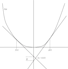
β(y)
(x,−α(x))
f(x) g(x)
2
[image:10.595.160.426.219.487.2]x
Figure 1: The relationship between the various quantities which can be derived fromβ. The pointsf(x) andg(x) are two values in the horizontal direction such that the difference in the slope ofβat these two points is 2, and such that these tangents intersect at a point with horizontal coordinate x. The height of the intersection point is−α(x), andγ(x) is such that the slopes of the tangents areγ(x)±1.
The key insight is that the best way is to find suitable β is via its convex dual. The construction begins with a convex function G(x) normalised such that
G(0) = 0 = G′(0−). Set φto be the increasing function given (where G′ is well defined) by φ(x) =G′(x), and defineβ via
β(y) = sup
x {xy−G(x)}; (2)
note thatφ= (β′)−1. ThenG(x) =xφ(x)−β(φ(x)) and
g(x) =φ(γ(x) + 1) f(x) =φ(γ(x)−1). (3)
From the definition ofLandg we have
= g(x)−x−α(x)−β(g(x))−γ(x)(x−g(x))
= (1 +γ(x))φ(1 +γ(x))−β(φ(1 +γ(x)))−α(x)−x(1 +γ(x))
= G(γ(x) + 1)−x−α(x)−xγ(x). (4)
Similarly,
0 =L(x, f(x)) =G(γ(x)−1) +x−α(x)−xγ(x) (5)
and subtracting these last two expressions we obtain
2x=G(γ(x) + 1)−G(γ(x)−1). (6)
If we then define H andγ via
H(z) = (G(z+ 1)−G(z−1))/2; γ=H−1. (7)
then (6) holds. Note thatH is increasing so thatγ is well defined and increasing, and sinceβ′ and φare also increasing we have thatg andf are increasing.
Finally, adding (4) and (5) we find
α(x) =−xγ(x) +1
2[G(γ(x) + 1) +G(γ(x)−1)]. (8)
An alternative expression involvingβ is
α(x) = (g(x)−x)β′(g(x))−β(g(x)) (9)
= (f(x)−x)β′(f(x))−β(f(x)). (10)
For a given convex Gthis completes the construction of a trio (α, β, γ) for which
L(x, y) given by (1) satisfiesL≤0.
In determining (α, β, γ) it is convenient to assume thatGis continuously differ-entiable and strictly convex. However, this is by no means necessary, and the only issues are in choosing the appropriate inverseγ toH in (7), which then enters the definition ofα. The easiest way to determine the correct form for the quantitiesα
andγ (andf andg) is via the graphical representation in Figure 1.
Theorem 9 Let µ and ν be a pair of centred probability measures which are
in-creasing in convex order. Let G be convex with G(0) = 0 = G′(0−), and define
β ≡βG andα≡αG via (2) and (8), where γ≡γG is defined in (7). Then, for all
(X, Y)∈ M(µ, ν)
E[|Y −X|]≤
Z
α(x)µ(dx) + Z
β(y)ν(dy). (11)
Proof: We simply need to show that L(x, y)≤0. To see this, for y > x(the case
y < x is similar)
L(x, y)
= (y−x) +xγ(x)−1
Butβ(y)≥zy−G(z) for allz includingz= 1 +γ(x). Hence L(x, y)≤0. Thus, givenGwe have a bound onE[|Y −X|] of the form
E|Y −X| ≤
Z
α(x)µ(dx) + Z
β(y)ν(dy)
where α=αG andβ=βG.
Remark 10 The normalisation of Gsuch thatG(0) =G′(0−) = 0 is convenient, but not important. If instead we set ˜G(x) =G(x−c) +d, then we find ˜β(y) =
β(y) +cy−d, ˜γ(x) =γ(x) +c and ˜α(x) =α(x)−cx+d, so that the bound in (11) is unchanged. In finance terms, any super-replicating strategy that involves options positions at times T1 and T2 and a forward position over [T1, T2] can be trivially
modified by adding a long position at T1, a short position atT2 and an offsetting
forward position.
Remark 11 The construction begins with G and this is the primary object used to calculate g and f from (3). Combining these with µ we can deduce the law ˆ
ν = ˆνf,g,µ ofY:
ˆ
ν((−∞, y]) =P(Y ≤y) =µ((−∞, g−1(y)]) +
Z f−1(y)
g−1(y)
g(x)−x
g(x)−f(x)µ(dx) (12)
Alternatively, given the convex duality between β andG, we can also start withβ
as the primitive object. In this way we can choose convex functions G and initial laws µ so that there is equality in (11) and hence optimality, for a certain law ˆν. In this sense it is easy to produce examples for which the bound is tight. However, the real aim is to start with lawsµandν and to constructGand the bound. This will prove to be much harder.
Remark 12 Recall the definitions offandg, which for the purposes of this remark we assume to be differentiable. Then they satisfy a certain consistency condition. From (3) we have
β′(g(x))−1 =γ(x) =β′(f(x)) + 1 (13)
and so
β′′(g(x))g′(x) =f′(x)β′′(f(x)) (14)
Also, from (9) and (10) we obtain
β(g(x))−g(x)β′(g(x))−(β(f(x))−f(x))β′(f(x))+x(β′(g(x))−β′(f(x)) = 0. (15)
Using (13), differentiating, and then using (14) we get
2
g(x)−f(x)=β
′′(g(x))g′(x) =f′(x)β′′(f(x)) (16)
so that in the appropriate domains
β′′(y) = 2
and
β′′(y) = 2
g′(g−1(y))(y−f(g−1(y))). (18)
Alternatively we can rewrite (15) as
0 = Z g(x)
f(x)
(y−x)β′′(y)dy (19)
which after substituting with (17) and some manipulations yields
0 =
Z f−1(y)
g−1(y)
(g(z)−f−1(y))
g(z)−f(z) dz. (20)
Substituting using the first inequality in (16), then changing variable and integrat-ing, and finally using (13) we obtain
Z x
g−1(f(x)) 2
g(z)−f(z)dz= Z g(x)
f(x)
β′′(y)dy= 2, (21)
so that
1 =
Z f−1(y)
g−1(y)
1
g(z)−f(z)dz, (22)
and then (20) is equivalent to
Z f−1(y)
g−1(y)
g(z)
g(z)−f(z)dz=f
−1(y) (23)
with a related expression interchanging the roles of f and g.
y=x
y=f(x)
[image:13.595.112.389.299.430.2]y=g(x)
Figure 2: A representation of functionsf andg.
β we will only recover the originalf and g if (23) holds. Equations (22) and (23) play the role of global consistency conditions on the functionsf, gwhich determines whether they are associated with optimal constructions. Note that it is a non-local condition in that it relatesf andgover whole intervals and not at isolated points. We will use this consistency condition to select the optimal solution (f, g) from the many which lead to embeddings.
Remark 13 The bound is attained if Y ∈ {f(X), g(X)}, or equivalently if the stopping rule τ is of the form τ =τ(f, g, B0) = inf{u: Bu ∈ {f(B0), g(B0)}}. In
that case we have an alternative representation of the bound7 as
2E
(g(X)−X)(X−f(X)) (g(X)−f(X))
, (24)
at least in the case where µ and ν have densities andf, g and their inverses are continuous and differentiable. The expression (24) follows directly from the fact that P(Y =f(x)|B0=x) = (g(x)−x)/(g(x)−f(x)). This expression can also be
derived via calculus from (12) using the definitions ofαand β.
6
Examples
6.1
Example: Quadratic functions
G
(
x
) =
x
2/
2
k
.
In this case β(y) = ky2/2, H(z) = z/k, γ(z) = zk, α(x) = (1−k2x2)/2k. We immediately recover the result in the opening remarks of Section 4: E[|Y −X|]≤
kE[Y2−X2]/2 + 1/2k. This result can be optimised by appropriate choice ofk.
We haveg(x) =x+k−1 and f(x) =x+k−1. Ifk= 1 and µ∼U[−1,1], then
recalling that ˆν(f, g, µ) = L(Bτ :B0 ∼µ, τ = inf{u >0 :Bu ∈ {f(B0), g(B0)}}),
we have that ˆν ∼U[−2,2] andH(µ,νˆ) = 1.
6.2
Example: Entropy
For this example it is natural to assume that X and Y are non-negative random variables, scaled to have unit mean.
TakeG(x) =Aex/ξ. Then
β(y) =ξ(ylny−yln(A/ξ)−y)
γ(w) =ξln(w/Asinh(1/ξ))
and
α(x) =−ξ(xlnx) +ξxln(Asinh(1/ξ)) +xcoth(1/ξ)
The bound is
E[|Y −X|]≤E[β(Y) +α(X)] =ξE[YlnY −XlnX] +J(ξ)
7
Observe thatf(x)≤x≤g(x) and so (g(x)−x)(x−f(x))/(g(x)−f(x))≤min{g(x)−x, x−
where
J(ξ) =ξlnξ−ξ+ξln(sinh(1/ξ)) + coth(1/ξ).
Note thatJ is a decreasing convex function on R+, with J(0) = 2. (The fact that
J(0) = 2 corresponds to the trivial boundE|Y −X| ≤E|Y|+E|X|= 2.) Let ˜J be the convex dual toJ, so that
˜
J(z) = inf
ξ>0(ξz+J(ξ)).
Then
Proposition 14 Let X and Y be positive random variables each with unit mean
and such that E[Y|X] =X. Suppose thatE[Y lnY −XlnX]≤∆. Then
E|Y −X| ≤J˜(∆).
The bound is tight, in the sense that for each ∆>0 there exists a pair(X, Y)with
E[Y lnY −XlnX] = ∆ for whichE|Y −X|= ˜J(∆).
Corollary 15 We haveJ(ξ)≤min{1/(2ξ),2}, and thenJ˜(z)≤√2z∧2. It follows
that E|Y −X| ≤√2∆∧2.
Corollary 16 IfX andY satisfy the hypotheses of Proposition 14 but have mean
c thenE|Y −X| ≤cJ˜(∆/c).
Note that, unlike in the quadratic example, the pre-multipleAplays no role in the final bound. Note further that as for the quadratic example, αtakes the same functional form asβ, so we get this very nice inequality involving the entropies of the two distributions. This makes the resulting inequality particularly attractive, but is a special feature of these examples.
We discuss the financial implications of this bound in Section 10 below. For this example we have thatg(x) =xe1/ξ/(ξsinh(1/ξ)) andf(x) =xe−1/ξ/(ξsinh(1/ξ)).
Both these functions are linear which makes it particularly simple to construct examples where the bound is attained. If X has an exponential distribution, then the construction yields Y which is a mixture of two exponentials.
6.3
Example: Multiplicity of Embeddings
Supposeµ∼U[−1,1] andν∼U[−2,2]. We know from Example 6.1 thatH(µ, ν) = 1, and that for the optimal constructionf(x) + 1 =x=g(x)−1. Our goal in this example is to show that this is not the only pair (f, g) for which ˆν(f, g, µ) =ν.
Fixa∈(−1,1) and suppose we have increasing functionsf : [−1,1]7→[−2, a] andg: [−1,1]7→[a,2]. For ˆν(f, g, µ) to equalν we must have
g′(z) = 2(z−f(z))
g(z)−f(z), f
′(z) = 2(g(z)−z)
g(z)−f(z).
Define va(z) = (4−4az+a2)1/2. Then, recallg(−1) =a=f(1) andg(1) = 2 =
−f(−1), g(z) = z+a/2 +va(z)/2 andf(z) =z+a/2−va(z)/2. For eacha ∈
constructions can be associated with the embedding which maximises E|Y −X|, and this will be the one for whichf andg satisfy the global consistency condition.
We can define a candidateβ from (19) and then β′′(y) =w
a(y) wherewa(y) =
(1−ay+a2)1/2. However, if we consider (20) fory=awe get
Z f−1(a)
g−1(a)
g(x)
(g(x)−f(x))dx= Z 1
−1
x+a/2 +va(x)/2 va(x)
dx= 1 +2 3a
This is equal to f−1(a) = 1 if and only if a = 0, so that out of the many pairs
(f, g) which embed (µ, ν) only the pair defined from a = 0 is consistent with a construction based upon a convex functionβ.
7
Constructing bounds given the marginals
In the previous section we derived upper bounds onE[|Y−X|] by considering fami-lies of functions derived from a convex functionG. There is a one-to-one relationship betweenGandβ, and so from either it is possible to deduce expressions forαand
γ, and thence, at least in the regular case where Gand β are smooth and strictly convex, we can obtain expressions for the monotonic functions f and g. Finally, conditional on the lawµforX we can find a bound forE[|Y −X|].
The construction gives a bound for any feasible law ν of Y but the bound is attained only for a particular lawν = ˆν(f, g, µ).
The issue is to reverse this construction, and given µand ν to find Gor β for which we can construct a best bound. Alternatively, given µ and ν we want to minimise the right-hand-side of (11) overGand more especially to prove this gives the lowest possible upper bound onH(µ, ν). A related problem is to find functions
f(x)< x < g(x), such that a construction of the formY ∈ {f(X), g(X)}is optimal for the problem. This is complicated by the fact that it is not sufficient simply to find f, g such that if X ∼ µ and both E[Y|X] = X and Y ∈ {f(X), g(X)} then
Y ∼ν.
Lemma 17 Supposef, g are strictly increasing, continuous and differentiable and
f, g solve (22) and (20). Then ifβ is given by the solution of (16),Gis the convex
dual ofβ andα=αG then
H(µ, ν) = Z
α(x)µ(dx) + Z
β(y)ν(dy).
where ν= ˆν(f, g, µ).
Proof: Given f and g satisfying (22) and (20) we can define β via (16), or the equivalent expressions (17) or (18). Given that (17) and (18) define β′′ in two different ways it should be checked that these two definitions do not lead to an inconsistency or self-contradiction. In fact differentiation of (22) shows that (17) follows from (18) and vice-versa.
It follows from (20) and (17) that
0 = Z g(x)
f(x)
Integrating the right-hand-side it follows that (15) holds and we can define α
via either (9) or (10). From the equivalence of these two representations (and
β′′(g(x)g′(x) = β′′(f(x)f′(x)) we deduce as in (21) that 2 = β′(g(x))−β′(f(x)). Letγ(x) =β′(g(x))−1 =β′(f(x))+1, then we have a tripleα, β, γ. Moreover, since the tangents to β at f(x) andg(x) intersect at (x,−α(x)) it is clear that when we defineφ(γ(x) + 1) andφ(γ(x)−1) we recoverg andf respectively. By hypothesis,
τ(f, g, µ) embedsν so thatH(µ, ν) =H(µ,νˆ(f, g, µ))≥R
α(x)µ(dx) +R
β(y)ν(dy), the inequality following from the fact that H(µ, ν) is a supremum over all embed-dings. The reverse inequality follows from Theorem 9.
The lemma provides a partial result, but it still remains to show that it is possible to findf, g which solve (22) and (20) and the embedding condition (12). It seems very difficult to exhibitf, g which solve this problem. Instead we will approximate
ν with a discrete distribution for which we can prove that an appropriate function
β exists, and derive the required result by taking limits.
8
Optimal upper bounds
The goal of this section is to find the value ofH(µ, ν) for arbitrary measures onR+, by finding an upper bound, and by showing the bound is attained. The approach is to begin with a point mass µand a discrete measure ν, and to progress to the full problem via a series of extensions.
8.1
The discrete case: preliminary results
Suppose thatX∼µandY ∼ν (withµν) are discrete, centred random variables with finite support. Denote the atoms by µi =µ({xi}) andνj =ν({yj}), where
the points{xi} and{yi} are ordered such thatx1< x2 <· · ·< xm andy1< y2<
· · · < yn. The problem is to find sup(X,Y)∈M(µ,ν)E|Y −X|. In this simple setting
this can be written as a finite linear programme:
max
ρij
X
i,j
ρij|yj−xi|
(25)
subject to the constraints
X
j
ρij =µi,
X
i
ρij =νj,
X
j
ρij(xi−yj) = 0, ρij ≥0. (26)
The associated dual problem is to find
min
αi,βjγi
X
i
αiµi+
X
j βjνj
,
where αi, βj, γi are chosen to satisfyL(xi, yj)≤0 for alliandj, where, in turn,
L(xi, yj) =|xi−yj| −αi−βj−γi(xi−yj).
By the complementary slackness condition we have that for an optimumρijL(xi, yj) =
Given the constants βj we can define a function β(y) via β(yj) = βj and by
linear interpolation between these points, with β(y) = ∞ outside [y1, yn]. Then
also we can defineL(xi, y) =|xi−y| −αi−β(y)−γi(xi−y).
The primal problem is feasible and therefore has a solution and the values of the primal and dual problems are equal, (for this fundamental result see Gale, Kuhn and Tucker [9], or for a recent treatment Vanderbei [19]).
Lemma 18 The solution of the linear programme is such that β(y)is convex iny
and γi is increasing ini. Further, if yj > xi andρij >0 thenρkl = 0 for all(k, l)
for which (k < i, l > j) and if yj < xi and ρij >0 then ρkl = 0 for all(k, l) for
which (k > i, l < j).
Proof: Supposeβ(y) is not convex. Then for somej∈ {2, . . . , n−1}
βj > βj+1 (yj−yj−1)
(yj+1−yj−1)
+βj−1 (yj+1−yj)
(yj+1−yj−1)
.
Fix i and suppose first that xi ≤ yj. Then from the fact that L(xi, yk) ≤ 0 for k=j±1 we obtain
βj+1 ≥ αi−(1 +γi)xi+ (1 +γi)yj+1
βj−1 ≥ αi−(1 +γi)xi+ (1 +γi)yj−1
and we conclude that βj > αi−(1 +γi)xi+ (1 +γi)yj. Hence L(xi, yj)<0 and ρij = 0.
A similar argument (but replacing (γi+ 1) with (γi−1)) applies ifxi> yj and
thenρij = 0 for alli. HencePiρij = 0, a contradiction.
Now consider the monotonicity of γ. We want to show that if xk > xi then γk > γi. We consider two cases depending on whether (xk,−αk) lies above or
below the tangent toβ with slopeγi+ 1.
Suppose (xk,−αk) lies strictly below the line y=−αi+ (1 +γi)(x−xi). This
condition can be rewritten as (αi+xi(1 +γi))<(αk+xk(1 +γi)).
We know there existsy > xk for whichL(xk, y) = 0. (In particular, there exists ρkj >0 for which the associatedyj > xk and thenL(xk, yj) = 0.) Then
0 =L(xk, y) = (y−xk)(1 +γk)−αk−β(y)
= [(y−xi)(1 +γi)−αi−β(y)] + [(y−xk)(γk−γi)]
+[(αi+xi(1 +γi))−(αk+xk(1 +γi))].
The first and last of the square-bracketed terms are negative sinceL(xi, y)≤0 and
by the hypothesis that (xk,−αk) lies below the tangent, and henceγk > γi.
If (xk,−αk) lies at or above the line y=αi+ (1 +γi)(x−xi), then it must lie
strictly above the tangent toβwith slopeγi−1, so we must have (αi+xi(γi−1))>
(αk+xk(γi−1)). Then by a similar argument to before we find for somey < xk
that 0 =L(xk, y)>(xk−y)(γi−γk).
Finally, supposeρij >0 foryj > xi andρkl >0 for (k > i, l < j). We want to
obtain a contradiction. By definition,
= ((yj−xk)(1 +γk)−βj−αk) + ((yl−xi)(1 +γi)−βl−αi)
= L(xi, yj) +L(xk, yl) + (γk−γi)(yj−yl)
= (γk−γi)(yj−yl)>0
The reverse case for yj< xi is similar.
In the discrete case, β is piecewise linear or equivalently β′′ is a purely atomic measure. For this reasonφ≡(β′)−1is not uniquely defined and the same applies to
f andg. For this reason we need an alternative parameterisation. The same issue can arise whenever µ has atoms, and in these cases it is convenient to introduce some independent randomisation.
Define FX(x) =µ((−∞, x]) and let U be a uniform random variable on [0,1].
Then FX−1(U) ∼ µ, and our approach for considering the case where X is not a continuous random variable is to condition on U rather than X, and to define a trio of increasing functions, p < q < r with domain [0,1]. In particular, we suppose B0 ≡X =q(U) (so thatq ≡FX−1), and we try to find p: [0,1]7→Rand r: [0,1]7→Rsuch that if
τp,q,r= inf{t:Bt∈/ (p(U), r(U))|B0=q(U)} (27)
thenY ≡Bτ ∼ν. The relationships betweenf, g andp, rare that f≡p◦q−1and g≡r◦q−1.
The embedding condition (recall (12)) becomes
ν((−∞, y]) = Z 1
0
duI{r(u)≤y}+
Z 1
0
duI{p(u)≤y<r(u)}
r(u)−q(u)
r(u)−p(u) (28)
Note that he embedding condition is easiest to express in terms of the functionsp, q
and r, whereas it is more natural to describe the ‘global consistency condition’ as conditions on f andg.
8.2
The discrete case: determining
p, q
and
r
for the case of
constant
X
Suppose that µ =δx, the unit mass at x. If ν =δx then we take p(u) = q(u) = r(u) =x. Otherwise, suppose thatY has law meanxand takes valuesyk1 < . . . <
ykm < x≤yj1 < . . . < yjn with probabilitiesνk1, . . . , νkm andνj1, . . . νjn.
The aim is to construct increasing functions p(u) < x < r(u) such that if
U ∼ U[0,1] and τ(u) = inf{s ≥ 0 : Bs ∈ {p(u), r(u)}} then Bτ(U) ∼ ν. (The
resulting construction is the analogue of Skorokhod’s original solution of the SEP, Skorokhod [17]).
The construction proceeds by induction: clearly if m = 1 = n, then we take
p ≡ p(u) = yk1 and r ≡ r(u) = yj1 and the martingale condition forces νj1 =
(x−yk1)/(yj1−yk1). Note that in this case
E|Y −X|= 2(r−x)(x−p) (r−p) = 2
Z 1
0
(r(u)−x)(x−p(u))
r(u)−p(u)
du.
So suppose m+n >2. Letu1= (yj1−yk1) min{νj1/(x−yk1), νk1/(yj1−x)}.
p(u)
q(u)
r(u)
u= 0 u= 1
y1 y2 y3 y4 y5 y6
[image:20.595.158.430.105.348.2]x1 x2 x3 x4
Figure 3: The functionsp, q, rin the discrete case. In this example the measureνplaces mass on{y1<· · ·< y6}andµplaces mass on{x1<· · ·< x4}.
νj1/(x−yk1)≤νk1/(yj1−x). (This will necessarily be the case ifyj1 =x.) Then
P(Y =yj1, U ≤u1) =u1(x−yk1)/(yj1−yk1) = νj1 and P(Y = yk1, U ≤ u1) =
u1(yj1−x)/(yj1 −yk1)≤νk1. Conditional onU ≤u1 we have embedded the mass
atyj1 and some of the mass atyk1, and so conditional onU > u1we must have that
Y does not take the valueyj1. Since,U conditioned onU > u1is again a uniform
random variable we can use the inductive hypothesis to complete the construction. In this way we construct increasing functions pand r with p(0) = yk1, p(1) =
ykm, r(0) = yj1, r(1) = yjn. It also follows that E[|Y −X|] = u1E[|Y −X||U ≤
u1] +E[|Y −X|;U > u1], and applying the inductive hypothesis to the latter we
again get
E|Y −X|= 2 Z 1
0
(r(u)−x)(x−p(u))
r(u)−p(u)
du.
8.3
The discrete case: determining
p, q
and
r
for the case of
general
X
The extension to random variablesX taking finitely many values is straightforward — ifX =q(U) then conditioning on the valueX =xis equivalent to conditioning on q−1(x−) < U ≤ q−1(x+) — and then the solutions for individual x can be pasted together. The results of Lemma 18 concerning where the joint measure ρ
places mass are sufficient to ensure thatrandpfrom this concatenation of solutions are increasing.
con-struction Y ∼ν. For the optimalp, rwe have
H(µ, ν) = 2E
(r(U)−q(U))(q(U)−p(U)
r(U)−p(U)
.
In particular, if
µ=
m
X
i=1
µiδxi, ν=
n
X
j=1
νjδyj,
then let (η(ji))1≤j≤n be the distribution on{yj}1≤j≤n given byηj(i) =ρij/µi. For
each iwe use the solution of Section 8.2 to produce functions pi(u)< xi < ri(u),
such that, if B0(i)∼δxi,Ui ∼U[0,1] andτi(u) = inf{s≥0 :B
(i)
s ∈/ (pi(u), ri(u))}
thenB(τi()Ui)∼η(i).
Now, withq=FX−1 andU ∼U[0,1], we definepandrvia
(p(u), r(u)) =
pi
u
−P
l<iµl µi
, ri
u
−P
l<iµl µi
X
l<i
µl< u≤
X
l≤i µl.
Then, the condition from Lemma 18 thatyj < xi andρij >0 impliesρi+1,l= 0 for l < j ensures thatpandr so defined are increasing.
8.4
General bounded measures by approximation
The idea to cover general centred measures is to approximate µ andν with finite measuresµmandνm. For these discrete problems we find the associated increasing pm, qm, rm. We have to show that these sequences converge and that the limits p, q, r are associated with a construction which embedsν and is optimal.
Suppose that X and Y have bounded support, and suppose µm and νm are
the approximations forµ and ν with support 2−mZ(recall Section 2 whereηm is
defined as an approximation ofηfrom above), and letpm, qm, rmbe the associated
increasing functions, the construction of which is as described in Section 8.3. For each fixedmthe pair (Xm, Ym) attainsH(µm, νm).
By Helley’s Selection Theorem (eg Billingsley [2]) there exists a subsequence down which each of pm, qm, rm and their inverses converge to p, q, r, p−1, q−1 and
r−1, at least at points of continuity of the limit functions. WritePmfor the inverse
to pm with similar expressions forqm, rm, p, qandr.
We have that
νm((−∞, y]) =
Z 1
0
duI{rm(u)≤y}+
Z 1
0
duI{pm(u)≤y<rm(u)}
rm(u)−qm(u) rm(u)−pm(u) (29)
and that νm((−∞, y])→ν((−∞, y]) at least at continuity points ofν. Moreover,
Z 1
0
duI{u≤Rm(y)}→
Z 1
0
duI{u≤R(y)}
sinceRm(y)→R(y) and
Z 1
0
duI{pm(u)≤y<rm(u)}
(rm(u)−qm(u)) rm(u)−pm(u) →
Z 1
0
duI{p(u)≤y<r(u)}
(r(u)−q(u))
since the limit function has only countably many discontinuities, and except at these discontinuities the integrand converges (and is bounded). It follows that (28) is satisfied, andτ=τp,q,rembeds ν.
It remains to show that this construction is optimal. Even if it is not we have the bound
H(µ, ν)≥E[|Bτ−B0|] = 2E (r(U)
−q(U))(q(U)−p(U))
r(U)−p(U)
. (30)
On the other hand, by Lemma 4,H(µ, ν)≤lim infH(µm, νm). But
H(µm, νm) = 2E
(rm(U)−qm(U))(qm(U)−pm(U)) rm(U)−pm(U)
→ 2E
(r(U)−q(U))(q(U)−p(U))
r(U)−p(U)
by bounded convergence, so there is equality throughout in (30).
8.5
Distributions on
R
+.
The final task is to extend the results of the previous section from bounded measures to measures on R+. Observe that results for centred distributions with bounded support extend by translation to any pair of distributions with bounded support and the same mean.
Suppose thatµandν have support onR+, and that both have mean c. From the put-call parity relation we have|Y−X|= 2(X−Y)++ (Y −X) and
so
ˆ
H(µ, ν) := sup
(X,Y)∈M
E[(X−Y)+]
satisfies ˆH(µ, ν) =H(µ, ν)/2.
For eachnset ˜X(n)=X∧nand ˜Y(n)=Y ∧λ(n) whereλ(n) is chosen so that
E[ ˜X(n)] =E[ ˜Y(n)]. It can be shown thatλ(n)≥n. Then for any joint distribution
of (X, Y) we have
E(X−Y)+= lim
n↑∞E[(X−Y)
+I
{X<n}] (31)
and
E[(X−Y)+I{X<n}] = E[( ˜X(n)−Y˜(n))+I{X˜(n)<n}] ≤ E[( ˜X(n)−Y˜(n))+]
≤ Hˆ(µ(n), ν(n)), (32)
where IA denotes the indicator function of the setAandµ(n)andν(n)denote the
laws of ˜X(n) and ˜Y(n). Both ˜X(n)and ˜Y(n)are bounded random variables and so
by the results of the previous section,
ˆ
H(µ(n), ν(n)) = Z 1
0
(r(n)(u)−q(n)(u)(q(n)(u)−p(n)(u))
for appropriate functions 0≤p(n)(u)≤q(n)(u)≤r(n)(u). Then
(r(n)(u)−q(n)(u)(q(n)(u)−p(n)(u))
(r(n)(u)−p(n)(u)) ≤q (n)(u)
−p(n)(u)≤q(n)(u)≤q(u).
This last inequality follows by construction, sinceqandq(n)are inverse distribution
functions ofX and ˜X(n)respectively.
Down a subsequence if necessary we have that p(n) and r(n)converge topand
rsay, and then by dominated convergence
ˆ
H(µ(n), ν(n))→
Z 1
0
(r(u)−q(u)(q(u)−p(u))
(r(u)−p(u)) du. (33)
Combining (31), (32) and (33) we conclude that the right hand side of (33) is an upper bound for ˆH(µ, ν). Moreover, by the same limiting arguments as before, p,
q andrdefine a feasible construction of a random variableY and hence
H(µ, ν) = 2 Z 1
0
(r(u)−q(u)(q(u)−p(u)) (r(u)−p(u)) du
as required.
We have proved:
Theorem 19 Suppose thatµandν are probability measures onR+each with mean
c, and suppose thatµν in convex order. LetU be a uniform random variable on
[0,1].
There exist increasing functionsp, q, rsuch thatX =q(U)andY ∈ {p(U), r(U)}
withE[Y|U] =E[X|U]satisfyX ∼µ,Y ∼ν andE[Y|X] =X, and the pair(X, Y)
is such that H(µ, ν) =E[|Y −X|]. Moreover,
H(µ, ν) = 2 Z 1
0
(r(u)−q(u))(q(u)−p(u))
r(u)−p(u) du.
If µ has no atoms then there exist increasing f and g such that X ∼ µ, Y ∈
{f(X), g(X)} with E[Y|X] = X satisfy Y ∼ ν and the pair (X, Y) is such that
H(µ, ν) =E[|Y −X|]Moreover,
H(µ, ν) = 2
Z (g(x)−x)(x−f(x))
g(x)−f(x) µ(dx).
Further, iff andgare strictly increasing, continuous and differentiable, then ifβ is
given by (17)-(18), and thenαis defined fromβas in Section 5, then an alternative
expression is
H(µ, ν) = Z
β(y)ν(dy) + Z
α(x)µ(dx)
Proof: The first part of the theorem was proved at the beginning of this section, and the second part follows immediately from the identification f ≡ p◦q−1 and
g =r◦q−1, note that the hypothesis is sufficient to ensure that q−1 is continuous
9
Numerical examples
In this section we present results from two numerical examples. In the first case we consider a pair of (continuous) uniform random variables and in the second case we consider a pair of normal random variables. The first step in each case is to approximate the initial and target random variables with discrete random variables. The problem of determining the joint law which maximises the expected value of
E|Y −X|can then be reduced to a finite linear programme of the form (25)-(26). The results of these programmes are presented in Figures 4 and 5 in the form of the associated functions f and g. In particular, it is implicit in these figures that the linear programme has found a solution where eitherY =f(X) orY =g(X) for increasing functions f andgas required by the analysis of Section 4.
−0.1 −0.05 0 0.05 0.1 −0.2
−0.15 −0.1 −0.05 0 0.05 0.1 0.15
Price at time 1
Price at time 2
[image:24.595.164.405.291.485.2]uniform, vol = (10%, 15%), #nodes = (40, 200)
Figure 4: The functionsy=f(x) andy=g(x) for a numerical example in whichX ∼
U[−0.1,0.1] andY ∼U[−0.15,0.15]. In fact both random variables are approximated by discrete uniform random variables on 40 and 200 points respectively. The linear programme
finds an optimum which places mass at a ‘cloud’ of points on a grid; these points have been smoothed to improve the clarity of the figure.
10
Efficiency of the bound in the lognormal case
Suppose that X and Y have lognormal distributions. In particular suppose thatµ
andν are the laws of
ceσ√T1G1−σ2T1/2 and ceσ√T2G2−σ2T2/2
respectively, for a pair of standard Gaussian random variablesG1 andG2.
A candidate martingale model for which the prices satisfyFT1 ∼µandFT2 ∼ν
is the Black-Scholes model
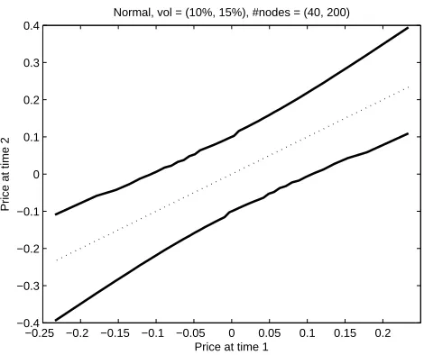
−0.25 −0.2 −0.15 −0.1 −0.05 0 0.05 0.1 0.15 0.2 −0.4
−0.3 −0.2 −0.1 0 0.1 0.2 0.3 0.4
Price at time 1
Price at time 2
[image:25.595.168.403.110.307.2]Normal, vol = (10%, 15%), #nodes = (40, 200)
Figure 5: The functions y = f(x) and y = g(x) for a numerical example in which
X ∼N(0, σ2
X) andY ∼N(0, σ 2
Y) whereσX= 0.1 andσY = 0.15. Both random variables
are approximated by discrete random variables such that X is approximated with a dis-tribution consisting of 40 atoms, andY is approximated by a random variable with 200 atoms.
Under that (complete market) model the price E ≡ E(V) for the forward start straddle is given by
E(V) =E[|FT2−FT1|] = E[FT1]E[|FT2/FT1−1|]
= cE[|eσ√T2−T1G−σ2(T2−T1)/2−1|]
= 2cP(−√V /2≤G≤√V /2)
where V = σ2(T2 −T1) and G is standard Gaussian. When V is small this is
approximatelyE(V)=. c√Vp 2/π.
Now consider the upper bound on the price of the option across all models which are consistent with the marginal distributions and the martingale property. We are going to use the entropy criterion to give a bound on H(µ, ν). Since the family of lognormal distributions is closed under multiplication, we might hope that the entropy bound is moderately tight. It can be shown that for lognormal distributions it always outperforms the bound based on quadratic functionals and the Cauchy-Schwarz inequality.
We have
E[Y lnY −XlnX] =cV 2 ; and then by Corollaries 15 and 16
H(µ, ν)≤cJ˜(V /2)≤c√V .
model-based price we find that the ratio of the prices satisfies
1≤HE(µ, ν(V)) ≤ J˜(V /2)
4Φ(√V /2)−2.
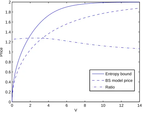
The model-based price, the entropy-based upper bound and the ratio of these quantities are plotted in Figure 6. Note that the smallest upper bound H is a function ofσ2T
1andV ≡σ2(T2−T1) whereas both the Black-Scholes model-based
price and the entropy-based bound depend on V alone.
0 2 4 6 8 10 12 14 0
0.2 0.4 0.6 0.8 1 1.2 1.4 1.6 1.8 2
V
Price
[image:26.595.172.407.245.432.2]Entropy bound BS model price Ratio
Figure 6: A plot ofE(V) (the Black-Scholes model-based price, dashed line) and ˜J(V /2) the entropy-based bound (solid line), scaled such that c = 1. The ratio between these prices is also shown; for small V the limit ratio is p
π/2, for largeV the limit is 1. We have 0 ≤E(V) ≤H(µ, ν)≤J˜(V /2)≤2∧√V. It should be noted that most plausible parameter combinations are represented by low values ofV, so the left-hand side of this figure is the most relevant.
Consider two agents (of different sexes) who wish to price a forward start straddle and who are in a market with vanilla call and put prices which are consistent with lognormal distributions for the asset price. The first agent assumes that prices follow a Black-Scholes model and charges E(V). If he delta-hedges the straddle, and if the price realisation is consistent with the constant volatility model then he will hedge perfectly. The second agent makes no modelling assumptions. She charges a higher price for the straddle (but at worst 30% higher, and typically less) and uses the premium to purchase a portfolio of puts and calls and atT1makes an
investment in the forward market. Under optimal portfolio choice, then whatever the realisation of the price process she will super-replicate.
References
[1] J. Az´ema and M. Yor. Une solution simple au probl`eme de Skorokhod. In
S´eminaire de Probabilit´es, XIII (Univ. Strasbourg, Strasbourg, 1977/78), pages
90–115. Springer, Berlin, 1979.
[2] P. Billingsley.Probability and Measure. Wiley, New York, second edition, 1986.
[3] D.T. Breeden and R.H. Litzenberger. Prices of state-contingent claims implicit in option prices. The Journal of Business, 51(4):621–651, 1978.
[4] H. Brown, D. Hobson, and L. C. G. Rogers. Robust hedging of barrier options.
Math. Finance, 11(3):285–314, 2001.
[5] R.V. Chacon. Potential processes. Trans. Amer. Math. Soc, 226:39–58, 1977.
[6] A.M.G. Cox and J. Ob l´oj. Model free pricing and hedging of double barrier options. 2008.
[7] M.H.A. Davis and D.G. Hobson. The range of traded options prices.
Mathe-matical Finance, 17(1):1–14, 2007.
[8] H. F¨ollmer and A. Schied. Stochastic Finance; An Introduction In Discrete Time. de Gruyter, 2004.
[9] D. Gale, H.W. Kuhn, and A.W. Tucker. Linear programming and the theory of games. In T.C. Koopmans, editor, Activity Analysis of Production and
Allocation, pages 317–329. Wiley, New York, 1995.
[10] D. G. Hobson. The Skorokhod Embedding Problem and model-independent prices for options. 2009.
[11] D.G. Hobson. Robust hedging of the lookback option.Finance and Stochastics, 2:329–347, 1998.
[12] D.G. Hobson and J.L. Pedersen. The minimum maximum of a continuous martingale with given initial and terminal laws. Annals of Probability, 30:978– 999, 2002.
[13] S. D. Jacka. Optimal stopping and best constants for Doob-like inequalities. I. The casep= 1. Ann. Probab., 19(4):1798–1821, 1991.
[14] J. Ob l´oj. The Skorokhod embedding problem and its offspring. Probability
Surveys, 1:321–392, 2004.
[15] E. Perkins. The Cereteli-Davis solution to theH1-embedding problem and an
optimal embedding in Brownian motion. In Seminar on stochastic processes,
1985 (Gainesville, Fla., 1985), pages 172–223. Birkh¨auser Boston, Boston, MA,
1986.
[16] D. H. Root. The existence of certain stopping times on Brownian motion.Ann.
[17] A. V. Skorokhod. Studies in the theory of random processes. Translated from the Russian by Scripta Technica, Inc. Addison-Wesley Publishing Co., Inc., Reading, Mass., 1965.
[18] P. Vallois. Quelques in´egalit´es avec le temps local en zero du mouvement brownien. Stochastic Process. Appl., 41(1):117–155, 1992.


![Figure 4: The functions y = f(x) and y = g(x) for a numerical example in which X ∼U[−0.1, 0.1] and Y ∼ U[−0.15, 0.15]](https://thumb-us.123doks.com/thumbv2/123dok_us/9627324.465264/24.595.164.405.291.485/figure-functions-numerical-example-x-u-y-u.webp)