Control of active cell balancing systems : innovation report

(1)

warwick.ac.uk/lib-publications

A Thesis Submitted for the Degree of PhD at the University of Warwick

Permanent WRAP URL:

http://wrap.warwick.ac.uk/108625

Copyright and reuse:

This thesis is made available online and is protected by original copyright. Please scroll down to view the document itself.

Please refer to the repository record for this item for information to help you to cite it. Our policy information is available from the repository home page.

(2)

Control of Active Cell

Balancing Systems

Innovation Report

Thomas Michael Bruen

EngD (International)

(3)

Abstract

Lithium-ion battery packs are increasingly being used for high power and energy applications such as electric vehicles and grid storage. These battery packs consist of many individual cells connected in series and/or parallel. Manufacturing tolerances and varied operating conditions mean that each cell will be different one from another, being able to store different amounts of energy and deliver different amounts of power. This also means some cells will finish charging or discharging before others, resulting in unutilised energy in the remaining cells.

Passive balancing systems are often used in multi-cell battery packs to ensure that all of the cells can be fully charged. However, this does not account for differences in cell capacity, meaning that not all cells will be fully discharged. Active balancing systems have been developed to transfer energy between the cells, in theory allowing for stronger cells to compensate for weaker ones. However, their perceived cost and complexity have prevented them from being widely adopted in commercial applications.

(4)

Acknowledgments

Firstly, I’d like to thank James Marco for supervising this research. Your advice, regular feedback and, most importantly, enforcement of deadlines made this work possible.

Thanks also to Paul Haney, Miguel Gama, Sue Slater and everyone in the JLR team for their support, opportunities and experience. I hope you can make the most of this research. I’d like to acknowledge the EPSRC and JLR for funding the project. The wider WMG centre HVM Catapult (refrerred to throughout this report as Catapult) has been instrumental in gathering the large volumes of test data used throughout this work.

I’m grateful to everyone who put aside time for technical discussions, notably Dhammika Widanalage and Mark Tucker, and to Andrew Moore and John Palmer for their assistance with laboratory work.

To my friends and family: thanks for your encouragement and distraction this past four years.

(5)

iii

Declarations

I declare that the work in this document is my own unless otherwise stated.

(6)

List of Figures

Figure 1: Unavailable energy owing to imbalance in series connected cells ... 2

Figure 2: Structure of the EngD Portfolio and Innovation Report... 5

Figure 3: Portfolio Submissions as a systems "V" diagram ... 6

Figure 4: Lithium-ion cell ageing mechanisms- from [30] ... 10

Figure 5: Capacity variation within battery packs - from [19] ... 13

Figure 6: Variations in cell ageing within EV battery modules – from [46] ... 14

Figure 7: Comparison of SOC imbalance and charge imbalance ... 20

Figure 8: ΔSOC metrics based on the mean, maximum and minimum SOC ... 23

Figure 9: Schematic of two cell imbalance distributions ... 29

Figure 10: A transformer-based pack-cell system - from [95] ... 30

Figure 11: Dual balancing system – from [98] ... 31

Figure 12: SOC balancing using model predictive control - from [108] ... 34

Figure 13: High-level summary of balancing control system components ... 39

Figure 14: ECM with 1 RC pair ... 41

Figure 15: Example OCV-SOC curves obtained using GITT for a nickel-cobalt-aluminium cell ... 45

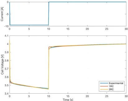
Figure 16: Example pulse power test current and voltage ... 47

Figure 17: Example pulse power fit results for 1 and 2 RC ECMs ... 49

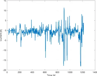
Figure 18: Catapult Validation Current Profile ... 50

Figure 19: Measured and simulated cell voltage during validation profile ... 51

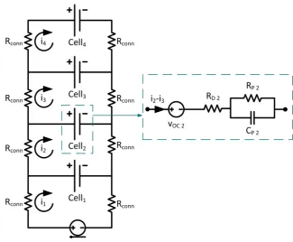
Figure 20: Schematic of four cells connected in parallel ... 54

Figure 21: Current junction (left-hand) and voltage loop (right-hand) in the parallel cell model ... 54

Figure 22: Example profile used to calibrate shunt resistors ... 58

Figure 23: Experimental and simulated current for four cells in parallel using 10Hz parameterisation data ... 59

Figure 24: Experimental and simulated current for four cells in parallel using 100Hz parameterisation data ... 61

Figure 25: Experimentally measured current and temperature during a 1C constant discharge ... 64

Figure 26: Simulation results for the validation drive cycle ... 66

(10)

Figure 28: Relative charge throughput for a 70p1s pack with interconnection

resistance ... 69

Figure 29: Example pulse power fit for an automotive pouch cell... 72

Figure 30: OCV-SOC data for an automotive pouch cell ... 73

Figure 31: Example model validation for an automotive pouch cell ... 74

Figure 32: Cell Voltages and SOCs during a 10 second pulse simulation ... 75

Figure 33: Artemis Combined drive cycle vehicle speed and derived battery current ... 76

Figure 34: Simulation of Artemis Combined drive cycle ... 76

Figure 35: Overview of the battery system in the context of balancing ... 81

Figure 36: Balancing Decision Flowchart ... 86

Figure 37: Example code for bisection algorithm... 98

Figure 38: DSIC imbalance removal ... 102

Figure 39: US06 drive cycle speed and current... 105

Figure 40: Rule-based logic while under a drive cycle load ... 106

Figure 41: Pole placement using SVD under no load ... 107

Figure 42: Pole placement using least squares under no load ... 108

Figure 43: Pole placement while under a drive cycle load ... 109

Figure 44: DSIC while under a drive cycle load ... 110

Figure 45: Feed-forward control while under a drive cycle load ... 111

Figure 46: Arrangement of balancing sub-modules ... 117

Figure 47: Simplified circuit diagram of one transformer ... 118

Figure 48: Simulation of the primary and secondary currents arising from converter switching ... 119

Figure 49: Balancing current as a function of cell and module voltages ... 120

Figure 50: Schematic of voltage measurements within series-connected cells ... 124

Figure 51: Balancing system wiring ... 125

Figure 52: Comparison of Cell 1 voltage and current for the combined and separate harnesses ... 125

(11)

ix Figure 55: Schematic of delayed voltage measurements during a dynamic current

profile ... 129

Figure 56: Histograms of cell voltage measurement noise for the NI 9219 module ... 130

Figure 57: Wire voltage calibration results ... 132

Figure 58: Schematic of final experimental configuration ... 135

Figure 59: Equipment set-up in the laboratory... 136

Figure 60: Repeated single-cell balancing ... 138

Figure 61: Single cell balancing experiment ... 139

Figure 62: Cell currents measured during the balancing permutation test ... 141

Figure 63: Evaluation of balancing system under external load ... 143

Figure 64: SOC and duty cycle results for pole placement under no load ... 145

Figure 65: Cell currents and SOCs for pole placement under Artemis Combined drive cycle ... 146

Figure 66: ΔSOC and absolute SOC difference for pole placement under Artemis Combined drive cycle ... 147

Figure 67: Cell currents and SOCs for DSIC under Artemis Combined drive cycle ... 148

Figure 68: ΔSOC and absolute SOC difference for DSIC under Artemis Combined drive cycle ... 149

Figure 69: Simulation results for pole placement under the US06 drive cycle 150 Figure 70: Simulation results for DSIC under the US06 drive cycle ... 151

Figure A- 1: Example EIS data of a cylindrical lithium-ion cell ... 180

Figure A- 2: ECM for EIS data ... 181

Figure A- 3: Example EIS results and model fit ... 183

Figure A- 4: Management of real-time closed loop system ... 186

(12)

List of Tables

Table 1: Summary of total imbalance measures for example cells... 23

Table 2: Sources of error from coulomb counting... 24

Table 3: Summary of ECM parameterisation results ... 49

Table 4: Parallel Cell Ageing Results ... 57

Table 5: Validation of current shunt measurements ... 59

Table 6 : Comparison of error between simulated and experimental data for various models ... 62

Table 7: Parameterisation Dataset for parallel cell ECMs ... 62

Table 8: Summary of parallel cell current distribution simulation results ... 68

Table 9: Summary of ageing characteristics of automotive pouch cells ... 72

Table 10: Pulse power ECM fit results for an automotive pouch cell ... 73

Table 11: Pouch Cell model validation results ... 74

Table 12: Battery subsystem descriptions ... 82

Table 13: Subsystems relating to cell balancing... 83

Table 14: Sources of error in control model ... 99

Table 15: Initial SOC vectors at different DODs ... 105

Table 16: Energy loss during balancing simulations... 112

Table 17: CAN message to specify balancing for one cell ... 122

Table 18: Wire voltage calibration results ... 132

Table 19: Current and efficiency for single-cell balancing ... 140

Table 20: Discharge balancing results for cells 3 and 4 ... 142

Table 21: Difference in balancing currents while under external load ... 143

Table 22: Summary of experimental test conditions ... 144

(13)

xi

List of Abbreviations

Abbreviation Full term

ABS Active Balancing System ADC Analogue-Digital Converter BEV Battery Electric Vehicle BMS Battery Management System DOD Depth of Discharge

DSIC Dynamic Steady-Input Control ECM Equivalent Circuit Model

EIS Electrochemical Impedance Spectroscopy EOC End of Charging

EOD End of Discharging EV Electric Vehicle

GITT Galvanostatic Intermittent Titration Technique HEV Hybrid Electric Vehicle

LQR Linear-Quadratic Regulator JLR Jaguar Land Rover

MPC Model Predictive Control OCV Open Circuit Voltage PBM Physics Based Model PCB Printed Circuit Board

PHEV Plug-in Hybrid Electric Vehicle PWM Pulse Width Modulation

RC Resistor Capacitor SIL Software-in-Loop SOC State of Charge SOE State of Energy SOH State of Health

(14)

Mathematical Notation

Notation Description Units

𝑨 State-space system state matrix -

𝑩 State-space system input matrix (Ah-1₎

𝑩𝒄 State-space system controlled input matrix (Ah-1)

𝑩_𝒅 State-space system disturbance input matrix (Ah-1₎

𝑩𝟏 State-space augmented system input matrix (Ah-1)

𝒃_𝟐 State-space augmented system disturbance vector (Ah-1₎ 𝑩(_𝟏 State-reduced state-space augmented system input

matrix

-

𝒃(_𝟐 State-reduced state-space augmented system

disturbance vector

-

𝑪 State-space system output matrix -

𝑪_𝒑 Cell polarization capacitance, as part of an impedance

model

Farads (F)

𝒅 Disturbance (uncontrolled) input to a system -

𝜹 The error between a measured and

simulated/estimated value

-

𝒆 The error between a measured and

simulated/estimated value

-

𝑬_𝒑𝒔 Parallel cell current calculation state matrix -

𝜼_𝒄𝒉𝒈 The efficiency of a balancing system for a charging

current

-

𝜼𝒅𝒄𝒉 The efficiency of a balancing system for a discharging

current

-

𝒇 Cost function scalar term -

𝒇_𝒑𝒔 Parallel cell current calculation input vector Ohms (Ω)

𝑭 Balancing current coupling matrix -

𝒈 Cost function linear vector -

𝑮_𝒅 Disturbance-output transfer function -

𝑮𝒑𝒔 Parallel cell current calculation current matrix -

𝑮𝒕𝒇 Input-output transfer function -

(15)

xiii

𝒊 An arbitrary current Amperes

(A)

𝒊_𝒂𝒑𝒑 The current applied to a battery pack Amperes

(A)

𝒊_𝒃𝒂𝒍 The current generated by balancing Amperes

(A)

𝒊_{𝒄𝒆𝒍𝒍} The current through a cell Amperes

(A)

𝒊_𝒇𝒃 The feedback current generated through active cell

balancing

Amperes

(A)

𝒊_{𝒍𝒐𝒐𝒑} The current within an electrical circuit mesh Amperes

(A)

𝒊𝒏𝒐𝒓𝒎 The current through a cell, normalised against applied

current

%

𝑰 Identity matrix -

𝒋 Angular frequency Rads-1

𝑱 Optimization cost function value -

𝑲 State feedback gain matrix -

𝑳 Kalman gain matrix -

𝒍𝒃 Optimization lower inequality constraint vector -

𝒎 Difference of cell SOC from the battery pack mean %

𝑴 Balancing s-to-m transfer matrix -

𝑵𝒎 The number of cells in series in a module -

𝑵_𝒔 The number of states in a system -

𝒐𝒏𝒆𝒔 A Matrix composed of elements of the value 1 -

𝒒_𝒄𝒂𝒑 Cell charge capacity

Ampere-hours (Ah)

𝒒_𝒃𝒂𝒍 Balancing charge Coulombs

𝑹𝒊𝒏𝒕 Cell internal resistance, found by applying a 10s

current pulse to the cell

Ohms (Ω)

𝑹𝑫𝑪 Cell internal resistance, at the point where the

complex component of impedance is zero

Ohms (Ω)

𝑹_{𝒄𝒐𝒏𝒏} Connection resistance between cells Ohms (Ω)

𝑹_𝟎 Cell internal resistance, as part of an impedance

model

(16)

𝑹𝒑 Cell polarization resistance, as part of an impedance

model

Ohms (Ω)

𝑹_𝒑𝒔 Parallel cell current calculation resistance matrix Ohms (Ω)

𝒔 Cell SOC %

𝑺𝑶𝑯_𝑬 State of Health with respect to energy %

𝑺𝑶𝑯_𝑷 State of Health with respect to power %

𝑺𝑶𝑪 State of charge %

𝒕 time Seconds (s)

𝝉_𝒑 impedance time constant Seconds (s)

𝑻 m-to-z transfer matrix -

𝒖 Controlled input to a system -

𝒖𝒃 Optimization upper inequality constraint vector -

𝑼𝑭 Battery pack energy utilisation factor -

𝒗_𝒐𝒄 Cell open circuit voltage Volts (V)

𝒗𝒑 Cell polarization voltage, for an impedance model Volts (V)

𝒗_𝒕 Cell terminal voltage Volts (V)

𝑾_𝒓 The winding ratio of a transformer -

𝒗 Generic dynamic system process noise vector -

𝒘 Generic dynamic system input noise vector -

𝒙 Generic dynamic system state vector -

𝒚 Generic dynamic system output vector -

𝒛 Balancing control system state vector -

(17)

1 Introduction

Lithium-ion cells are increasingly being used for a variety of technologies, ranging from smartphones through to electric vehicles (EVs) and grid storage for renewable energy sources [1]. They offer around twice the energy and power density than nickel metal-hydride cells, and about four times that of lead-acid cells, opening up battery power to applications which were not feasible until recently. Lithium-ion cells can be comprised of a variety of different chemistries depending on requirements such as energy, power, lifetime and cost [2]. The main thing these cells all have in common is that the voltage is quite low. Generally when a cell is fully charged it will be circa 4V, and when it’s fully discharged it will be slightly under 3V. For some chemistries, the operating range is even lower. This is insufficient for an EV whose powertrain requires 300V or above [3, 4], and closer to 1000V for Formula E racing cars [5]. To reach these sorts of voltages, hundreds of cells need to be connected in series. Furthermore, cells connected in parallel may be required in order to store more energy or increase the power capability of the battery system. For example the 2016 Tesla Model S 100KWh battery pack contains 8256 cells [6]. This introduces a number of problems:

• All of the cells need to be packaged, electrically connected, monitored,

thermally regulated and controlled. The more cells there are, the greater the cost, complexity and weight.

• Manufacturing tolerances and varying operating conditions mean that

each of these cells will be slightly different. The amount of energy each one can store will differ, as will the amount of heat generated internally and the amount of charge lost over time through self-discharge.

Multi-cell battery packs can become quite complex and require a battery management system (BMS) to control them. This uses sensor information such as cell voltages, currents and temperatures to ensure the battery pack is in a safe state, as well as predict the cells’ energy and degradation levels.

(18)

before a higher capacity one. Conventionally there is no control over how individual cells are loaded which means when one cell is fully charged or discharged, the entire pack has to cease operation. Different combinations of capacities, and variations in energy levels, means that most cells will not be fully charged or fully discharged, resulting in unused areas of energy as shown in grey in Figure 1. The height of the cell represents how much energy it can store, and the alignment shows the differences in energy levels: at the point in time where one cell has 100Wh remaining, another cell may only have 80Wh remaining and as such is closer to the end of discharge (EOD). In other words, the battery pack is not storing as much energy as it could, and the energy it does store is not being completely used. If this battery pack could fully utilise its energy, it could be made smaller without compromising EV performance.

Figure 1: Unavailable energy owing to imbalance in series connected cells

Cells at different energy levels are described as “imbalanced”, and balancing systems have been developed to address this issue. Prior to li-ion technology this was straightforward, as the cells could be overcharged: the current was applied until the last cell reached the maximum voltage, and the other cells would settle at this maximum. However, it is dangerous to over-charge li-ion cells and so another means of balancing must be sought. The simplest way is to apply passive balancing: connecting a resistor over the cell. This will gradually discharge the cell according to Ohm’s law. Cells at higher energy levels can be discharged down to the same level as the cell with the lowest energy, and then charging can be completed. This simplicity comes with a number of drawbacks:

• The energy from passive balancing is wasted as heat dissipated by the

(19)

• The balancing current is generally low in order to limit the heat generation.

This means that balancing can take a long time, increasing the overall charging time of the battery pack.

• Even if the cells are all completely balanced by end of charge (EOC), the differences in capacity mean that some cells will reach EOD before others. The best case for passive balancing is that all of the energy of the weakest cell is utilised.

Active balancing is an alternative strategy which could address the downsides to passive balancing by using power electronics to move energy between cells. If one cell is going to reach EOD before another, it can be charged up by the other cells and similarly if one cell is going to reach EOC before the others, it can discharge into them. The energy is utilised by other cells rather than being dissipated as heat. While this can potentially offer significant performance benefits, there are some downsides. The cost is higher, and the electronics takes up extra space and adds new failure modes to the battery pack [7].

For these reasons, active balancing systems (ABSs) have not, to date, been adopted for any mass-production vehicle applications. However, Jaguar Land Rover (JLR), with whom this EngD is in partnership with, has not looked in-depth at the current state of active balancing systems, and more generally there is a lack analysis of active balancing systems within the context of a complete battery pack. The Research Problem that this EngD addresses is: while active cell balancing technology is available, there is little understanding of, or

agreement on, how it should be used, what specific problems it is

addressing, and how much benefit it can provide within a future EV

application.

(20)

1.1 Research Questions and Objectives

Several open research topics in the area of imbalance were identified after a preliminary analysis of the literature, including:

• What are the fundamental causes of cell-to-cell variation, and how can

they be reduced?

• Using large datasets from aged EV battery packs, can statistical models be generated which accurately predict the spread of imbalance over time for different applications and operating conditions?

• How can balancing hardware be further improved, particularly regarding

scaling up to a high voltage battery packs containing hundreds or thousands of cells?

• Can cost and size reductions be made to make load-regulating smart cells

feasible for near-future battery pack integration?

While these questions are apposite, the major observation from the literature review was that there does not appear to have been a thoroughly designed balancing control system, which factors in a high-level strategy, a low-level energy management scheme and adaptability to the many types of balancing hardware. The lack of a comprehensive active balancing strategy means that the potential benefits, such as increased energy output, have not been fully realised and so active balancing appears less cost effective than it could otherwise be. This EngD therefore aims to address the following Research Questions:

1. In what context can active balancing provide the greatest benefit? 2. What kind of gains in energy utilisation can be achieved using active

balancing, compared to passive balancing?

Question 1 considers the higher-level aspects of active balancing, such as if it is only suited to certain applications and whether parallel cells also require balancing. Question 2 uses the information from Question 1 to formulate a control strategy to maximise energy utilisation, which can be verified experimentally to quantify its performance. To achieve this, the following objectives were defined:

1. Define the sources of imbalance within a battery pack and the affect

(21)

2. Understand the current status of active balancing hardware and

evaluate their suitability for different applications.

3. Create a modelling framework to analyse imbalance and aid in

designing a control system.

4. Develop a generic balancing control system with the specific goal of

maximising the energy utilisation of the battery pack.

5. Implement the control system in real-time with specific balancing

hardware and evaluate its performance, including the gain in energy

utilisation.

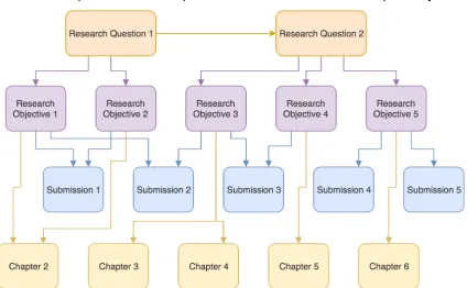
[image:21.595.117.542.373.635.2]

Figure 2 presents the relationship between the two Research Questions and the Research Objectives. In addition, Figure 2 highlights the relationship between each Research Question and the corresponding Portfolio Submission and Chapter within this Innovation Report. The structure of the Portfolio and Innovation Report are further explained in sections 1.2 and 1.3 respectively.

Figure 2: Structure of the EngD Portfolio and Innovation Report

1.2 Structure of the Portfolio

(22)

balancing systems, and some initial modelling of balancing systems. An IFAC conference paper was produced from this work, concerning high-level modelling and control of balancing systems [8]. Submission 2 documented the modelling and experimental work on cells connected in parallel. From this, a journal paper and conference paper were published [9, 10]. This work was also combined with some further modelling work related to [8], to publish another journal paper on multi-cell BMS applications [11] Submission 3 introduced the control model and used this to design and critically assess various options for feedback design. In Submission 4, the cells and balancing hardware used for experimental work was detailed, including the various iterations of the test set-up. The commissioning tests performed to analyse the system were documented. In Submission 5, experimental balancing tests were performed. Two of the controllers from Submission 3 were developed further, and state of charge (SOC) estimators were also designed to use as part of the control system. The controllers were run in real-time and their performance evaluated. The research Submissions should be read in their order of writing, as they follow a simplified systems “V” diagram as shown in Figure 3. The literature review in Submission 1 helped outline the performance criteria which would ultimately be validated via the experimental work in Submission 5.

Figure 3: Portfolio Submissions as a systems "V" diagram

1.3 Structure of the Innovation Report

(23)

(24)

2 A Review of Imbalance and Balancing

Two distinct literature reviews were conducted to understand the many aspects and research areas covered by energy imbalance. The first literature review, in section 2.1, addresses the first Research Objective of understanding which aspects of cell performance a balancing system can address, and what the benefits will be for the overall battery pack. It covers how cell-to-cell variations arise and what this means for battery pack performance, followed by an analysis of the impact each of these variations has on imbalance, and how imbalance should be defined. A second review was conducted in section 2.2 on the various means of transferring energy between cells, and existing control strategies for managing this energy transfer. This directly meets the second Research Objective of surveying the current status of balancing hardware. Conclusions are drawn in section 2.3.

2.1 Cell-to-Cell Variation

Each cell within a battery pack will have different properties to one another. These can be caused by intrinsic factors, for example limitations in the manufacturing process, or extrinsic factors such differences in operating conditions [12].

Fabricating cells is a complex, multi-step process [13, 14], and variations in properties arise from tolerances in these steps. Improving this process will reduce the size of the variations, which could reduce the amount of balancing required. However, it is not possible to remove variations completely, especially when there are often conflicting objectives such as the need to reduce the cost of manufacturing [14, 15]. In addition, new cell chemistries require different manufacturing techniques, and so there would likely be an increase in variation before these new processes are refined.

(25)

beneficial for excluding particularly weak cells but, ageing is open loop1_{so even} a very small initial imbalance will increase over time. There is also the growing second-life sector, in which aged cells are repurposed for other applications. For example, a cell which no longer has sufficient performance for its automotive application is still capable of delivering energy, and can be used as part of a grid storage system [19]. Nissan [20] and Renault [21] are both trialling energy storage units comprised of used automotive cells for homes with solar panels. This is essentially the opposite of screening: as the purpose is to make use of old cells, there will inherently be large variations in cell properties, and possibly even the types of cell.

Factors such as electrode thickness and porosity, and the amount of active material will affect cell properties [19, 22, 23]. There is generally a positive correlation between cell mass and cell capacity, as heavier cells should contain more active material [12, 24], but there is evidence that some variations in manufacturing affect mass but not capacity [25]. There is a lack of data on cell-to-cell variability, especially for automotive grade cells, but figures for the initial spread in capacity for cells from established manufacturers include 2-6% [26], 4% [25], 4.5% [19], 8% [27] down to about 1% after screening [28].

2.1.1 Cell Ageing

One of the key drivers of cell-to-cell variation over time is how the cells degrade (also known as ageing). Understanding and reducing cell degradation is one of the key challenges to overcome in the lithium-ion battery field. There are many causes of degradation, which are often complex and nonlinear in [29, 30]. Figure 4, reproduced from [30], shows how system-level inputs such as current and temperature cause a variety of chemical interactions which ultimately affect the two main systems-level metrics of cell degradation: capacity fade and power fade.

1_{There is some control over how cells age, such as the charging regime, specification of power}

(26)

[image:26.595.120.558.60.313.2]

Figure 4: Lithium-ion cell ageing mechanisms- from [30]

Capacity fade reduces the energy availability of the cell and is caused by a reduction in the amount of lithium available for cycling and a reduction in the space in the electrodes to store it. Power fade is caused by an increase in impedance: more of the power generated by the cell will be dissipated as heat, meaning that the efficiency drops and the cell cannot deliver as much power to the wider system. This leads to two common definitions of state of health (SOH): a 0-100% of cell degradation relative to when the cells were new. The energy SOH is defined by (1), and the power SOC defined by (2). Qcap is the cell capacity in ampere-hours, Rint is the internal resistance of the cell in ohms, and tf is the present time. Capacity and resistance are defined and discussed further in Chapter 3.

𝑆𝑂𝐻_[ = 100𝑞`ab

cdce

𝑞_`abcdf (1)

𝑆𝑂𝐻g = 100

𝑅_ijccdce

𝑅_ijccdf (2)

(27)

source of power alongside an internal combustion engine system. The latter ensures that range requirements are met, and the battery helps deliver sufficient power, as well as absorbing power through regenerative braking [35]. The battery pack must therefore be capable of high power, rather than delivering a large amount of energy. Conversely, for battery electric vehicles (BEVs) the battery pack is the only power source, and the dominant requirement is being able to delivery large amounts of energy (driving range), while the large pack size means the power demand is relatively low. Plug-in-hybrid electric vehicles (PHEVs) lie between the two, where there is still an engine, but unlike a HEV, the vehicle can be driven using battery power alone, and recharged from the grid as well as the engine. For HEVs, the SOHP criterion is more likely to be reached first, whereas

SOHE is the dominant factor for BEVs [33, 34]. Experimental results such as in [36, 37] demonstrate a correlation between SOHE and SOHP due to the overlap and interaction between the various ageing mechanisms. However, other studies show little correlation between resistance and capacity fade [38] which emphasises the complex nature of ageing, and the importance of analysing both

SOHP and SOHE and using the appropriate metric depending on the application.

Generally, higher temperatures increase ageing [39], with a general relationship that the rate of ageing doubles every increase of 10°C [34]. When the cells are

being cycled, cold temperatures also increase ageing via different mechanisms. Experimental results from [31] show that for cells under load, the primary cause of ageing below 25°C is lithium plating during charging, whereas degradation reactions and solid electrolyte interphase (SEI) growth occur above 25°C. High currents rates also increase ageing [40], with particularly high magnitudes inducing electrode fatigue and fracturing as the electrode expands and contracts during lithium insertion and removal [29]. High currents will also increase the cell temperature, potentially driving additional ageing as discussed above.

(28)

magnitude and temperature, so the BMS strategy may work to limit ageing in other ways (e.g. more conservative power limits). However, grid charging of BEVs offers more opportunity for cell balancing rather than a HEV, so cycle life may be improved. This DOD relationship is disputed by Peterson et al. [42] and Choi et al. [43] The latter compared different DODs but all started at 100% SOC rather than being centred about 50% SOC, so the tendency for a high SOC to accelerate ageing may factor into their results. The former results are based on vehicle drive cycles rather than typical laboratory cycling so the effects of the current profile on ageing may be tied to DOD ageing. This suggests that results from laboratory testing do not necessarily extrapolate to real-world vehicle usage. A higher mean SOC also tends to accelerate ageing due to the increased difference in potential between the electrodes and electrolyte [34, 39].

2.1.2 Battery pack ageing

While the causes of cell degradation are useful to understand, it is the cell-to-cell variation which is most relevant to balancing: even if the values are all poor from a performance point of view (e.g. a very high self-discharge rate), if all cells have the same value then the cells will still be balanced. One of the lesser studied areas of particular relevance for balancing high-voltage battery packs is a statistical analysis of how large numbers of cells age.

Baumhofer et al cycle-aged 48 pre-screened commercial Li-ion cells under the same operating conditions (current profile and ambient temperature) and measured cell capacity periodically [28]. Not only did capacity difference amongst the cells increase from 1% to 8%, there was no correlation between the initial and aged capacities: one of the lowest capacity cells when new ended up as one of the highest capacity cells after ageing, and vice versa (a result also observed in [44]). This means that screening is not a reliable indicator of cell performance long-term. The authors also found there was little correlation between relative resistance and capacity when new [45], which means that screening for capacity might result in a wide variation in impedance, and vice versa.

(29)

compare to 1908 aged cells from BEVs, taken from two different vehicles both driven regularly for three years. One important finding, reproduced in Figure 5, shows how the distribution of cell capacity changes with ageing. The distribution of the aged cells is noticeably skewed compared to the approximately normal distribution of the new cells. This means that outliers are much more likely to have a lower SOH than the mean (their results applied for both resistance and capacity). As battery pack performance is limited by the weakest cell, there will be a greater percentage of unused energy remaining in an aged pack

than a new one. The distributions between the two sets of aged cells is also

different. The cells from BEV 1 appear to have a bimodal distribution, with two peaks in the histogram, whereas BEV 2 has a more defined single peak. The authors note that BEV 2 was driven further and more aggressively, covering 26,745 km and consuming 19.0kWh/100km, compared 21397km and 16.9kWh/100km for BEV 1. This emphasises that long-term battery pack performance needs to be understood from a statistical point of view, as well as the physical basis behind the variation.

Figure 5: Capacity variation within battery packs - from [19]

(30)

[image:30.595.116.536.360.581.2]

A Weibull distribution for cell capacity was also observed in [38], in which the authors disassembled a battery pack from a vehicle driven for 32500km over 3 years in a city in southern China. The 95s5p (ninety-five units in series, each unit comprising five cells connected in parallel) battery pack had a nominal cell capacity of 12Ah, though the authors considered each parallel stack of series as a single cell with a 60Ah nominal capacity. The mean SOHE was 82.4%, with the maximum 4.4% above the mean and the minimum 8.7% below. In [46], an EV battery pack comprised of 50Ah pouch cell was disassembled after 30000km of driving. The authors found that the SOHE varied from 91 to 98% and, as Figure 6 shows, there was significant variation within each 10-cell module, as well as between each module. This shows that cell balancing just within modules is insufficient: reducing imbalance within module 13 has no impact on total driving range since module 11 would still limit battery pack operation.

Figure 6: Variations in cell ageing within EV battery modules – from [46]

(31)

module. However, there are several caveats to these results. Work co-authored by the author [37] demonstrated that the SOHs of cells connected in parallel will converge over time (and as such, not diverge if they were similar to begin with). As such, each module can be considered to contain 8 units with potentially different SOHs. This is a low number from a statistical point of view, especially considering the importance of outliers on overall performance, as discussed above. The same repeated drive cycle is not representative of real-world operation, and compressing ageing into 12 months does not account for how cells degrade with time. There is no information on the thermal design of the pack, such as any cooling system or ventilation. Ultimately, the statistical data from [27] and [46] give a better indication of the imbalance expected from EV operation, as they are obtained from actual EV modules. However, the results in [47] are still significantly different to other laboratory testing such as in [28], which may suggest that manufacturing standards are improving.

There is a consensus within the literature above that differences in cell temperature is a key driver of imbalance. As well as changing the rates of self-discharge between cells, it also causes greater variations in cell ageing, setting up a larger amount of imbalance in the future.

2.1.3 Drivers of Imbalance

Section 2.1 discussed the ways in which variations between cells arise. These variations can be considered within the context of imbalance specifically. There are three main properties which vary between cells: self-discharge rate, impedance and capacity [17, 48]. These variations are best considered at the different time-scales in which they create imbalance.

2.1.3.1 Long Term: Self-discharge

(32)

rate of self-discharge [51–54] owing to the Arrhenius relationship [54]. Additionally, self-discharge is known to be a function of SOC [49].

Self-discharge can be modelled as a small current perpetually discharging the cell [55]. However, a physical current is not actually generated external to the cell and so is not measured by a BMS. Depending on battery pack hardware design, some of the electronics powered by the cells themselves (such as monitoring and safety circuitry) may draw different amounts of current, thus acting in a similar manner to self-discharge when the battery pack is active [51].

Differences in self-discharge rates between cells mean that over time the SOCs of cells will diverge even if they were previously balanced. One of the advantages of Li-ion cells over other chemistries such as nickel-metal-hydride is the low self-discharge [1, 56]. Figures quoted include 1-10% SOC per month [49], 0.5-8% SOC per month [48], 6-10% SOC per month at 40°C, and 3-5% per month [57].

There is very little data concerning the spread of self-discharge between cells, but the consensus is that it will only induce significant imbalance over many days, meaning that cell balancing to counter this only has to be performed every few weeks [48].

2.1.3.2 Short Term: Capacity

(33)

Differences in capacity can arise through manufacturing variations, and the spread increases with ageing [27, 28] The imbalance induced through capacity differences is reversible, in that once the cells are recharged they will return to approximately the same state of balance as when discharging began. If balancing was performed during discharging, it would then have to be performed again during charging, which wastes energy and potentially increases the time to complete charging if balancing is slow.

The impact of capacity on overall performance is dependent on the application. For example, a HEV typically maintains the cells within a narrow SOC range, e.g. 40-60% SOC [41, 58, 59]. Differences in capacity will not affect battery pack performance significantly, because there is scope to widen the DOD window slightly if necessary. However, a BEV application might require using almost the entire SOC window. The Tesla Model S reportedly utilises 96% of the total available energy [60]. In this event, a relatively small divergence in cell capacities could reduce the energy availability of the battery pack to less than is required. This also increases the chances of the driver running out of range: SOC estimates are subject to some uncertainty, and that becomes more apparent when there is only a few percent SOC remaining.

2.1.3.3 Instantaneous: Impedance

(34)

In this sense, the weakest cell (from a capacity point of view) is not currently limiting pack performance. Derating strategies are often required to limit currents in low and high SOC regions to avoid cells undergoing loads which cause them to exceed these voltage [7, 61].

As well as increasing with ageing, a cell’s impedance is a function of temperature and SOC [58, 62]. A higher temperature reduces the impedance, improving efficiency at the expense of increasing ageing [63, 64]. Impedance also tends to increase at SOCs above 80-90%, and in particular at SOCs below 20-30% [64, 65]. An application which requires a wide DOD, such as a BEV, is likely to enter these regions. This reduces efficiency as more energy is dissipated as heat.

Cell voltage and impedance are at the core of imbalance within parallel connected cells. It is commonly assumed that energy balancing is only required for cells in series [17, 66] as the cells in a parallel unit are inherently balanced through being at the same terminal voltage [58, 67]. However, until recently there was little experimental data to explore this further. Following the work published by the researcher [10, 37], detailed in section 4.1, there has been more research into parallel connected cells, generally looking at the impact of temperature variations on parallel currents, the implications for the BMS, and better understanding the underlying cell properties which cause different currents [68– 71].

2.1.4 Quantifying imbalance

The literature review above has made clear that cell-to-cell variations have implications for overall battery pack performance, and a balancing system can mitigate against several aspects. In order to do this, imbalance must be quantified as a useable metric. The BMS can then analyse the imbalance status of each cell and decide on the nature of the corrective action to be taken.

2.1.4.1 Imbalance Metric

From a review of battery system operation, there are five potential measures which can form the basis of imbalance quantification:

(35)

• Charge

• Energy

• SOC

• State Of Energy (SOE)

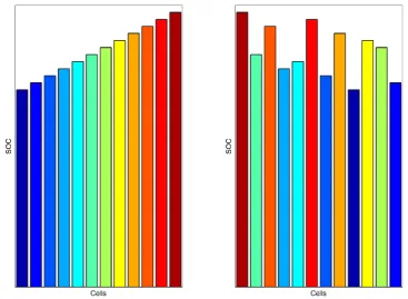
Charge level is perhaps the most logical reference point to evaluate imbalance. As discussed in section 2.1.3.2, imbalance arises during operation because cells in series can store different amounts of charge, but all undergo the same current. However, there are some issues with using charge. Firstly, it is an estimate, although this is true for all measures apart from voltage. A poor estimate means that the perceived imbalance is incorrect, and implementing the balancing strategy could lead to more imbalance. Secondly, as it is an absolute value, there is only one reference point. When all cells are fully discharged, they will all be at 0Ah charge, which means they are balanced. However, if all cells are fully charged, they will be at varying Ah levels owing to their different capacities. This implies a large amount of imbalance, but is actually desirable, so the imbalance metric needs to be recalculated depending on the direction of charge.

(36)

Figure 7: Comparison of SOC imbalance and charge imbalance

While charge and current are often the focus of discussions about cell performance, energy and power are ultimately what are required of a battery system. To achieve a certain power value, equation (3) shows that a higher current is required to compensate for a lower open circuit voltage (OCV). This means that for a BEV driver following a certain route, the battery pack SOC will decrease slower when the pack is fully charged compared to if it is only partially charged, even though the amount of energy used is the same2_{. The SOE would} change the same amount both times.

𝑃 = 𝑣_m`𝑖 (3)

From this perspective, state of energy (SOE) is a more representative metric for describing imbalance. However, SOE adds further complexity compared to SOC. The equation for SOC is linear, as it is simply accumulating current over time, and scaling by cell capacity (see Chapter 3 for a thorough derivation of cell state equations). SOE calculation must factor in how the OCV changes with the energy level, which is a nonlinear relationship. This nonlinearity makes control design more complex, while still ultimately being a similar imbalance metric to SOC.

Often, differences in cell voltage between cells is used to gauge imbalance [52, 72–74]. Voltage is a direct measurement, avoid issues with estimates. However, as mentioned in section 2.1.3.3, cells at the same charge or energy level can be at different voltages, because of their impedance differences. If the current direction changes, the cell at the highest voltage would become the cell at the lowest voltage, which from an imbalance perspective is confusing as it also reverses the state of imbalance. This also hints at another problem with voltage:

2_{In practice there will be slight differences in energy usage because the efficiency of the battery}

Cell

(37)

unlike the others metrics discussed here, it is not a state and changes instantaneously with current. This again complicates the control strategy. Consider some cells at rest, where one cell is at a slightly higher voltage than the others. The balancing controller sets it to discharge, to bring its voltage down to the same as the other cells. However, the application of the balancing current drops the cell voltage to approximately the same voltage as the other cells. This would imply it no longer needs to be balanced, but removing the balancing current would return the cell voltage to close to its original voltage, higher than the others.

Often balancing, especially passive balancing, takes place at or near EOC [7], where the current magnitude is relatively low and will not change direction. This can be considered a coarse approximation of OCV and so SOC (the relationship between OCV and SOC is discussed further in Chapter 3). However it is clear that under a dynamic load, voltage is an unusable metric for gauging imbalance, and unsuitable for control purposes. One relatively simple means of improving the voltage metric is to subtract the resistive voltage from the measured voltage

vt to obtain a more stable value vs using (4). This removes the most dynamic fluctuations in cell voltage. However, this has some drawbacks. The internal resistance estimate Rcell does not account for the full cell impedance and so some voltage dynamics are still present. Rcell is also an estimate, and as noted above varies significantly with SOC, temperature and ageing. This is similar to a common method of SOC estimation in which the impedance is modelled to predict vt [75, 76], but with a very simple impedance model and no corrective feedback to improve performance. As the BMS requires a SOC estimate for other purposes, it would be logical to use that SOC estimate rather than produce what is essentially a poorer version specifically for the balancing system.

𝑣_o = 𝑣_c− 𝑅_`qrr𝑖_`qrr (4)

(38)

this imbalance, but could mean the balancing system repeatedly being switched on and off without having an impact on imbalance. SOC offers a suitable compromise, with minor drawbacks being outweighed by its simplicity and estimation reliability compared to other metrics.

2.1.4.2 Relative imbalance

Whatever metric is used, its value has to be assessed relative to the other cells. There are two main options for doing this. The global difference for an SOC vector s (5) can be used, which gives a good indication of overall imbalance, but does

not give any indication of the state of imbalance amongst the cells, which then raises the question of how each cell should be controlled. Secondly, the distance from the mean m can be calculated, with the ith mean given by (6). This is useful when trying to determine a path for how all cells should be balanced, and the mean is a convenient reference. Alternatively, the distance of each cell from the maximum/ minimum cell could also be used. This would limit the balancing speed, as it would only occur in one direction, but may be applicable when the module of cells is near EOC/ EOD. For example, if the cells are being charged and are approaching EOC, then charging the strongest cells is not required: the priority is to bring all the cells up to the same level as the strongest. Taking the mean of the SOCs can be achieved with a constant matrix, whereas comparing to the maximum or minimum would require a change in function as different cells become the minimum/ maximum, causing discontinuities in the control process. Using this imbalance vector, the total imbalance can also be defined using the sum of squares (7). However, this is less relevant than (5) for describing total imbalance as it is the maximum and minimum that govern the overall pack performance.

imbalance = max(𝒔) − min (𝐬) (5)

𝑚_i = 1

N• 𝒔‚

‚

jdƒ

− s_… (6)

imbalance = •[𝑚]ˆ idƒ

(39)

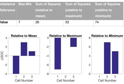
Consider the three cell SOC vector in (8). The ΔSOC vector based on the mean, maximum and minimum are shown in Figure 8. Table 1 shows these different measures for the example 3-cell SOC vector, s. The sum of squares is different depending on the measure, so is not as effective as an overview of total imbalance and would have to be recalibrated based on operating conditions.

[image:39.595.123.535.223.502.2]

𝒔 = [26 33 31] (8)

Table 1: Summary of total imbalance measures for example cells

Imbalance

Reference

Max-Min Sum of Squares

(relative to

mean)

Sum of Squares

(relative to

maximum)

Sum of Squares

(relative to

minimum)

Value 7 26 53 74

Figure 8: ΔSOC metrics based on the mean, maximum and minimum SOC

Based on the above discussion, the distance from the mean is best suited to an imbalance controller, and max-min imbalance used in the higher-level balancing control strategy, to assess the total state of imbalance.

2.1.5 SOC Estimation

(40)

in section 3.3.1. However, even this can be subject to error if the OCV-SOC data is incorrect or simplified owing to interpolation or averaging the charge and discharge OCV-SOC curves. SOC can be calculated using (17), also known as coulomb counting, but there are several sources of error in this equation as summarised in Table 2Error! Reference source not found..

Table 2: Sources of error from coulomb counting

Source Errors

Initial SOC s SOC is an integrator and so accumulates charge relative to a starting point. If the initial SOC is incorrect,

the future values will also be incorrect.

Current icell Errors in current can arise from incorrect calibration and quantisation. Additionally, discrete sampling means

that the sample taken is assumed constant for the

following time-step, when in practice it may differ.

Cell capacity Qcap The cell capacities well generally be an estimate and as such subject to some uncertainty. Incorrect

estimates will incorrectly scale conversion from charge

to SOC.

(41)

computationally expensive to execute. The literature suggests there is little difference in accuracy between the KF and data-driven methods.

2.1.5.1 Kalman Filter Framework

The KF is a commonly used algorithm for estimating states in physical systems and has been proven over time to be efficient and robust for a wide variety of applications [82–84]. The general data fusion method for a KF is outlined below. The ^ accent denotes that the variable is an estimate not a measurement, the - superscript indicates that the estimate is prior to correction, and the + superscript indicates the estimate is post correction. The k subscript denotes the relative point in time. The input vector u, state vector x, and process noise vector w are passed into the state update function to obtain the uncorrected state estimate at the next step using (9)Error! Reference source not found.. This is stored and used at the next time step. The uncorrected state vector, input vector, and output noise vector v are passed through the output function (10) to obtain an estimate of the measured output. The Kalman gain matrix Lk provides a systematic way of correcting the state estimates using the measurement data (11)Error! Reference source not found..

𝒙Œ_𝒌Ž𝟏• _{= 𝑓(𝒙Œ} ‘ Ž_{, 𝒖}

‘, 𝒘Œ‘) (9)

𝒚Œ_‘• _{= 𝑔(𝒙Œ} ‘ •_{, 𝒖}

‘, 𝒗Œ‘)

(10)

𝒙Œ_‘Ž _{= 𝒙Œ} ‘

•_{+ 𝐿}

‘(𝒚‘− 𝒚Œ‘•)

(11)

The specific calculation of L depends on the type of filter used. It is calculated according to two matrices: the state process noise matrix and output noise matrix. The process noise matrix indicates the accuracy of the model: small matrix values imply confidence in the model, meaning that the states will not be corrected much for a given measurement error, whereas larger values acknowledge that there are a number of model errors or unmodelled effects in Error! Reference source not found. [82]. Similarly, the output noise matrix indicates noise on the output

(42)

respectively, but in practice often become tuning factors whose values are adjusted until the desired performance characteristics are reached. One of the difficulties of the KF is that the v and w values are generally unknown and can vary with time, and often may not be Gaussian white noise as the filter assumes [82]. Implementation of a nonlinear KF for real-time SOC estimation is detailed in section 4.3.

2.2 Balancing Methods

A literature review was conducted on balancing hardware to understand the state of the art as well as future directions. There have been many proposed methods for active balancing, reviewed in section 2.2.1. Research into control of balancing systems is covered in section 2.2.2. The majority of the review focused on ABSs as there is little research to be done on passive balancing. Passive balancing involves discharging a cell by connecting a resistive load across its terminals. This is commonly used for commercial applications because of its low cost and [7, 73, 85]. However, there are several drawbacks:

• The discharging process wastes the energy – it is dissipated as heat.

• Balancing currents are typically low to avoid generating too much heat. Daowd et al. [73] suggest a maximum passive balancing current of C/100. Andrea [7] suggests 10-100mA for passive balancing depending on battery pack size. This means that balancing can take a long period of time. Even so, passive balancing may be limited owing to excessive heat generation [86]. Often the resistive loads for several cells are in a small, poorly ventilated box within the battery system where temperature rises can be significant. Moore and Schneider [74] deem the heat power generated by passive balancing large enough to cause costly thermal management requirements, even for a C/100 current rate.

(43)

Despite these drawbacks, there does not appear to be much use of active balancing at a production level. The Toyota Prius and McLaren P1 both use some form of active balancing, though few details are available [87]. Both vehicles are HEVs, and it may be that the battery packs are small enough to make integrating an active balancing system easy enough compared to a larger BEV pack. Linear Technology Corporation have developed a production-ready active balancing chip, the LTC 3300-1 [88], which can be used on battery packs over 1000V. This chip was used for experimental work in Chapter 6. General Motors patented an active balancing method which uses a DC-DC converter using the strongest cell to the weakest cell [89], though it is not clear if it has been used on a production vehicle.

2.2.1 Active balancing methods

(44)

One of the simplest methods of energy redistribution is using capacitive systems. A capacitor can act as a temporary energy storage medium between two cells: charged up by a higher voltage cell, and then discharged into the lower voltage cell. In [91], the authors recommend using ultracapacitors, whose low resistance can speed up balancing times. Despite this, the experimental results still show balancing taking 4 hours to remove 15% imbalance, which is relatively slow compared to other systems covered in this review. Sheng et al. [92] used cell-to-cell balancing using supercapacitors. As well as being used for equalization, the supercapacitors are also employed to absorb charge during a high-power event. By being in parallel with a cell, the total current is distributed between the cell and supercapacitor, reducing the load through the cell, which will help limit ageing. It is not clear from the paper how this is regulated; specifically, if the supercapacitors are maintained in a partially charged state such that they can accept and deliver large currents. An inductor can be used for cell-to-cell balancing in a similar way to capacitive systems, but the energy is stored in a magnetic field rather than an electric field [17]. The inductor size and switching frequency dictates how much charge is stored and the transfer rate between the cells.

(45)

[image:45.595.140.508.60.329.2]

Figure 9: Schematic of two cell imbalance distributions

A cell-to-cell balancing system would have to perform a series of balancing operations to pass the excess charge from the right-hand cells along to the weaker left hand cells. Each balancing operation between neighbouring cells will not reduce pack imbalance by much, and increases energy inefficiency. However, on the right-hand plot the imbalance distribution is random. In this case, there are generally high SOC cells next to low SOC cells and so there can be a significant reduction in imbalance through a single balancing operation between two neighbouring cells. Kim et al. [94] proposed adding additional switches and/ or capacitors to speed up the process, but this still lacks flexibility with regard to where energy can be moved to and from, and the amount of charge transferred is dependent on the relative cell voltages.

(46)

[image:46.595.203.463.103.401.2]

the secondary current to be established. In the paper only equalization of single cells is discussed, which could result in a slow balancing time.

Figure 10: A transformer-based pack-cell system - from [95]

A time-shared system is proposed in [96] in which a group of cells share a single cell-module flyback converter. Multiplexing is used to connect each cell to the converter for a short period of time. The authors emphasise that the system is made up of fewer components than most other ABSs. Despite this, it is was able to remove a 33% SOC difference between four 2.65Ah cells in 90 minutes. The main issue is how this is scaled up to a battery pack. As the converter is shared, the balancing speed will generally decrease as the number of cells increases, unless the power is increased.

(47)

cell, the balancing time will increase in proportion with the number of cells, making it much slower for an EV battery pack which can use over 100 cells in series.

Dual balancing systems have also been proposed, which separates imbalance at the cell and module level. Liye et al. [98] employ an inductive system to balance modules, and cell-to-cell capacitor system between the cells in each module. The schematic show in Figure 11 shows the modules E1 to En which can each be switched into the transformer circuit which in turn will charge the pack. The authors see it as being particularly suitable for a HEV drive cycle due to its ability to work during charge and discharge and not requiring a long period of time to balance, although there is no further justification of why it suits an HEV as opposed to other EVs. The results are not described in terms of balancing time or current so comparison with other systems is difficult.

Lin et al. [99] uses an inductive system to actively balance neighbouring modules, followed by dissipative balancing of the cells within each module. In [95], an extension is proposed to balance between modules in a similar way that cells within each module are balanced. None of the papers contains analysis on how much each system contributes to reducing the amount of imbalance or how much energy each system wastes through heat dissipation or inefficiency. Furthermore, analysis of the effectiveness of the dual balancing system as a function of pack and module size would offer greater insight into the benefits and limitations of such a system.

(48)

A similar two-layer approach is used in [100], where cell-to-cell balancing takes place within modules, and then the modules are balanced. As discussed above, cell-to-cell balancing becomes slower as the number of cells increases, so the performance depends on how the battery pack is subdivided into modules. In [101], the authors avoid having to split the system into modules. They use a DC-DC converter on each cell which all link to a common output bus for the low voltage system of an EV. The total applied load current can be distributed amongst the cells, with weakest cells undergoing less of the load. The hardware appears promising from a control perspective as it offers variable current allocation of each cell, but the problem of scaling the system up from the 3 cell demonstration to a full battery pack remains open.