Thermal Ignition Using Moving Hot Particles

(1)

Thesis by

Stephanie Alexandra Coronel

In Partial Fulfillment of the Requirements

for the Degree of

Doctor of Philosophy

California Institute of Technology

Pasadena, California

2016

(2)

c

2016

Stephanie Alexandra Coronel

(3)

(4)

Acknowledgements

I am incredibly grateful to my thesis advisor, Professor Joe Shepherd, for his guidance

and unwavering support over the past years. He has shaped who I am both as a

scientist and a person. By allowing, and even encouraging, me to work independently

in the laboratory I was able to hone my skills as an experimentalist, but, of course,

he also knew when to step in and provide useful counsel. Although he had other

commitments, previously as Dean of Graduate Studies and currently as Vice President

of Student Affairs, he always made time to advise and meet with me, including during

more evenings and weekends than I can remember. I cannot express enough how

thankful I am for his countless hours of help during this process, without which I am

certain I would not have successfully completed my PhD. I was extremely fortunate

to have had Professor Shepherd as an advisor and will always value his mentorship

and friendship.

I would like to thank the members of my thesis committee, Professors Joanna

Austin, Guillaume Blanquart, and Beverley McKeon, and also Professor Ravi

Ravichan-dran, who was part of my candidacy committee. I would especially like to thank Ravi

for his support and encouragement during my time at GALCIT.

I owe a debt of gratitude to past and present members of the Explosion Dynamics

Lab. I am thankful to Dr. Sally Bane, who mentored me when I came to Caltech

for an undergraduate summer internship in 2008 and later when I joined the research

group as a graduate student. She taught me the ins and outs of the laboratory,

and also provided words of encouragement when my research was not going so well.

She became a great friend and has been a source of inspiration throughout my time

(5)

Dr. Bane. I would also like to thank Drs. Philipp Boettcher and Jason Damazo.

They helped make my transition to the laboratory a smooth one and remain my

good friends. I also want to thank the current group members, Drs. Josu´e

Melguizo-Gavilanes and R´emy M´evel. They are supremely skilled researchers who have become

good friends and have helped to make my experience in the group so rewarding.

Their knowledge of chemistry and reactive flow simulations has been invaluable to

my work. I am grateful for their support and will truly miss our time together after

leaving Caltech. Finally, I will be eager to learn of the many accomplishments of

Jean-Christophe Veilleux as he continues his graduate studies and Bryan Schmidt as

he starts his career following commencement.

To the first year group of 2009, it was a pleasure to have shared the ups and downs

of the Master’s year. We formed friendships that year that remain strong to this day.

This group made the first year at Caltech incredibly fun; of course, the fun came after

all the problem sets were completed. Thank you especially to Jomela Meng, Ignacio

Maqueda, and Siddharta Verma; we had so many great times together and so many

laughs.

I am grateful to my mother, Betty Manno, her husband, Paul Manno, and my

siblings, Karol Trojacek and Alex and Marco Coronel, for their loving support. I

could not have done this without them. My mother was my inspiration for pursuing

graduate studies and through her endless encouragement and love I have been able

to complete this magnificent journey.

Finally, a loving thank you to Adam Wright. He is an incredible human being

and I am lucky to have met him. Thank you Adam for your patience, support, and

love throughout these years. I look forward to building our future together.

This work was supported by the Boeing Company through a Strategic Research

(6)

Abstract

In this work, ignition of n-hexane-air mixtures was investigated using moving hot

spheres of various diameters and surface temperatures. Alumina spheres of 1.8−6

mm diameter were heated using a high power CO2 laser and injected with an

av-erage velocity of 2.4 m/s into a premixed n-hexane-air mixture at a nominal initial

temperature and pressure of 298 K and 100 kPa, respectively. The 90% probability

of ignition using a 6 mm diameter sphere was 1224 K. High-speed experimental

vi-sualizations using interferometry indicated that ignition occurred in the vicinity of

the separation point in the boundary layer of the sphere when the sphere surface

temperature was near the ignition threshold. Additionally, the ignition threshold was

found to be insensitive to the mixture composition and showed little variation with

sphere diameter.

Numerical simulations of a transient one-dimensional boundary layer using

de-tailed chemistry in a gas a layer adjacent to a hot wall indicated that ignition takes

place away from the hot surface; the igniting gas that is a distance away from the

sur-face can overcome diffusive heat losses back to the wall when there is heat release due

to chemical activity. The use of fluid parcel tracking indicated that in an-hexane-air

mixture at Φ = 0.9, it was a fluid parcel located a distance of 0.15δT normal to the

wall that first ignited, where δT is the thermal boundary layer thickness. Finally, a

simple approximation of the thermal and momentum boundary layer profiles

indi-cated that the residence time within a boundary layer varies drastically, for example,

a fluid parcel originating at 0.05δT normal to the wall has a residence time that is

65× longer than the residence time of a fluid parcel traveling along the edge of the

(7)

A non-linear methodology was developed for the extraction of laminar flame

prop-erties from synthetic spherically expanding flames. The results indicated that for

accurate measurements of the flame speed and Markstein length, a minimum of 50

points is needed in the data set (flame radius vs. time) and a minimum range of 48

mm in the flame radius. The non-linear methodology was applied to experimental

n-hexane-air spherically expanding flames. The measured flame speed was

insensi-tive to the mixture initial pressure from 50 to 100 kPa and increased with increasing

mixture initial temperature. One-dimensional freely-propagating flame calculations

showed excellent agreement with the experimental flame speeds using the JetSurF

(8)

Published Content and

Contributions

Publications

J. Melguizo-Gavilanes, A. Nov´e-Josserand, S. Coronel, R. M´evel, and J. E. Shepherd.

Hot surface ignition of n-hexane mixtures using simplified kinetics. Combustion

Sci-ence and Technology, 2016c. Accepted for publication

J. Melguizo-Gavilanes, S. Coronel, R. M´evel, and J. E. Shepherd. Dynamics of

igni-tion of stoichiometric hydrogen-air mixtures by moving heated particles.International

Journal of Hydrogen Energy, 2016b. Accepted for publication

R. M´evel, J. Melguizo-Gavilanes, U. Niedzielska, S. Coronel, and J. E. Shepherd.

Chemical kinetics ofn-hexane-air atmospheres in the boundary layer of a moving hot

sphere. Combustion Science and Technology, 2016. Accepted for publication

Conference Proceedings

S. A. Coronel, S. Menon, R. M´evel, G. Blanquart, and J. E. Shepherd. Ignition of

nitrogen diluted hexane-oxygen mixtures by moving heated particles. In 24th

Inter-national Colloquium on the Dynamics of Explosions and Reactive Systems (ICDERS

2013), Taipei, Taiwan, 28 July-2 August 2013b

S. A. Coronel, R. M´evel, P. Vervish, P. A. Boettcher, V. Thomas, N. Chaumeix,

N. Darabiha, and J. E. Shepherd. Laminar burning speed of n-hexane-air mixtures.

In8th US National Combustion Meeting, University of Utah, May 19-22 2013c. Paper

070LT-0383

S. A. Coronel, V. Bitter, N. Thomas, R. M´evel, and J. E. Shepherd. Non-linear

(9)

Meeting, Western States Section of the Combustion Institute, California Institute of

Technology, March 24-25 2014. Paper 087LF-0020

S. A. Coronel, J. Melguizo-Gavilanes, and J. E. Shepherd. Ignition of n-hexane-air

by moving hot particles: effect of particle diameter. In 9th US National Combustion

Meeeting, Cincinnati OH, May 17-20 2015. Paper 0114RK-0452

R. M´evel, J. Melguizo-Gavilanes, S. A. Coronel, and J. E. Shepherd. Chemical

kinet-ics of ignition ofn-hexane by a moving hot sphere. In25th International Colloquium

on the Dynamics of Explosions and Reactive Systems (ICDERS 2015), Leeds, UK,

August 2-7 2015

S. A. Coronel and J. E. Shepherd. Effect of equivalence ratio on ignition and flame

propagation of n-hexane-air mixtures using moving hot particles. In 25th

Interna-tional Colloquium on the Dynamics of Explosions and Reactive Systems (ICDERS

2015), Leeks, UK, August 2-7 2015

Stephanie Coronel designed, constructed and carried out the experiments

de-scribed in Chapters 2, 3, 4 and 7. Stephanie Coronel developed the software and

analyzed all experimental data presented in all Chapters. Josu´e Melguizo-Gavilanes

performed the 2D simulations presented in Chapters 3 and 4. Stephanie Coronel

per-formed the 1D numerical simulations presented in Chapter 5 with the assistance of

Simon Lapointe. The analysis in Chapter 6 was initiated by R´emy M´evel and Vaugh

Thomas; Stephanie Coronel developed the software, performed the simulations and

analyzed the results. The experiments and data analysis in Chapter 7 were

per-formed by Stephanie Coronel, the flame speed calculations were perper-formed by Simon

Lapointe. Stephanie Coronel was the sole author of all chapters in this thesis and

(10)

List of Figures

1.1 Photograph showing frictional sparks and hot spots produced during a

grinding test . . . 1

1.2 Micrograph of filled-hole specimen subjected to 30 kA simulated

light-ning strike . . . 2

1.3 Schematic of laminar flow with separation around a sphere . . . 5

1.4 Prandtl number as a function of temperature for n-hexane-air mixtures 5

1.5 Streamlines surrounding sphere for increasing Re flows . . . 6

1.6 Evolution of the momentum boundary layer around sphere for separated

flow . . . 7

1.7 Isotherms surrounding sphere for increasing Re flows . . . 8

1.8 Isotherms surrounding sphere for increasing particle size . . . 10

1.9 Ignition delay time measurements as a function of gas temperature . . 11

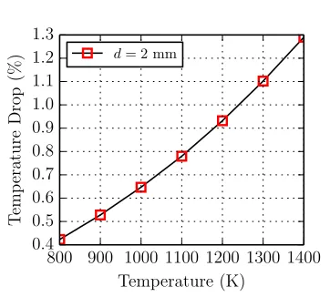
1.10 Temperature drop calculations during sphere falling time of 250 ms as a

function of initial sphere surface temperature for different sphere diameters 15

1.11 Temperature drop calculations for a 2 mm diameter sphere over 50 ms

(time interval between sphere entering the reactive mixture to ignition

taking place . . . 16

1.12 Previous experimental results of hot particle ignition in hydrogen-air

mixtures . . . 17

1.13 Previous experimental results of hot particle ignition in n-pentane-air

mixtures . . . 19

(17)

2.2 Configurations for heating spheres using electrical current and a high

power laser . . . 23

2.3 Sphere supports based on the configurations shown in Fig. 2.2 . . . 24

2.4 Experimental procedure for igniting a reactive mixture using a moving hot sphere . . . 25

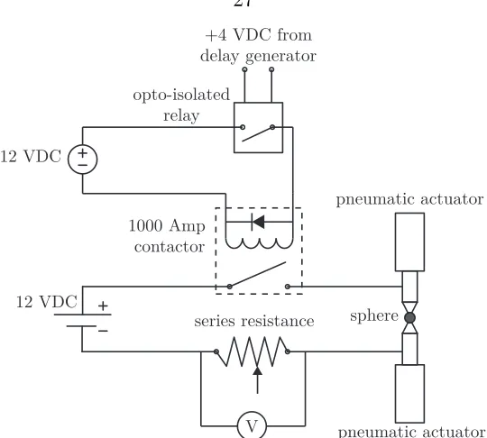
2.5 Circuit schematic for resistively heating small metallic spheres . . . 27

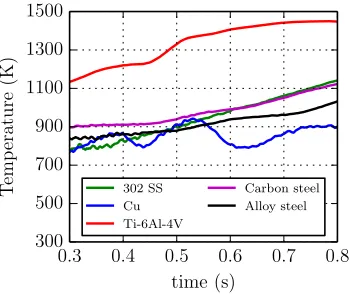
2.6 Timing diagram illustrating the experiment time and electrode retraction 27 2.7 Surface temperature of various resistively heated metal spheres mea-sured with two-color pyrometer . . . 28

2.8 Electrical heating of titanium alloy 4 mm diameter sphere in air at room temperature and pressure . . . 28

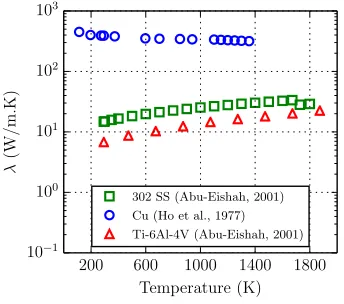
2.9 Thermal conductivity as a function of solid temperature . . . 29

2.10 Material properties as a function of solid temperature (electrical resis-tivity and specific heat) . . . 29

2.11 Beam splitting of CO2 laser beam . . . 30

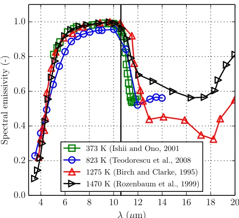
2.12 Timing diagram illustrating the laser controller and support retraction 31 2.13 Alumina spectral emissivity . . . 32

2.14 Blackbody spectral radiance at various temperatures . . . 34

2.15 Schematic of two-color pyrometer with one input fiber . . . 36

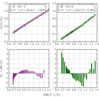
2.16 Calibration curves for fiber A and fiber B . . . 37

2.17 Schematic of two-color pyrometer with two input fibers . . . 38

2.18 Error in temperature for fiber A and fiber B as a function of ln V1/V2 38 2.19 Shearing interferometer schematic . . . 39

2.20 Wollaston prism schematic . . . 40

2.21 Orientation of beams separated by Wollaston prism . . . 41

2.22 Interference patterns for different β values . . . 41

2.23 Shearing interferometer layout used in testing . . . 42

2.24 Light wave passing through a radially symmetric medium . . . 47

(18)

2.26 Schematic of ray passing through a spherical hydrogen-air flame . . . . 49

2.27 δ versus the gas temperature for air at room temperature and

atmo-spheric pressure . . . 51

2.28 δ and dδ/dλ versus wavelength for air at room temperature and

atmo-spheric pressure . . . 52

3.1 Finite fringe and infinite fringe interferograms of thermal boundary layer

and wake surrounding falling hot spheres . . . 54

3.2 Infinite fringe interferograms of wake around hot spheres falling in n

-hexane-air . . . 55

3.3 Temporal evolution of a vertical slice taken at the sphere centerline of

the interferograms in Fig. 3.2 . . . 56

3.4 Reynolds number as a function of fluid temperature for three sphere

diameters and a fixed velocity of 2.4 m/s . . . 56

3.5 Kinematic viscosity as a function of gas temperature forn-hexane-air at

Φ = 0.9 and an initial temperature and pressure of 300 K and 100 kPa 57

3.6 Cold, film, and hot flow Reynolds number for spheres traveling through

n-hexane-air at 2.4 m/s . . . 57

3.7 Experimental and simulation comparison of n-hexane-air wake around

hot sphere (d= 6.0 mm) . . . 58

hot sphere (d= 3.5 mm) . . . 59

hot sphere (d= 1.8 mm) . . . 59

3.10 Interferogram of hot 6.0 mm diameter sphere with a surface temperature

of 1187_±18 K falling through air at 2.4 m/s (shot #110) . . . 61

3.11 Histogram of log|f| taken from the images in Fig. 3.10 . . . 61

3.12 2D intensity plot of log_|f_| taken from the images in Fig. 3.10 . . . 62

3.13 ∆ϕW along a vertical slice of the interferogram shown in Fig. 3.10 . . . 63

(19)

3.15 Phase demodulation of the Gaussian filtered interferogram using the

WFF2 method . . . 64

3.16 Time averaged unwrapped optical phase difference obtained from the phase demodulation of the original interferograms . . . 65

3.17 Time averaged unwrapped optical phase difference obtained from the phase demodulation of the Gaussian filtered interferograms . . . 65

3.18 Slices of ∆ϕat y= [1,2,5,10,15] mm as a function ofx . . . 66

3.19 Slices of ∆ϕat x= [−4,−1,0,2,4] mm as a function of y . . . 67

3.20 A slice of ∆ϕat y= 1 mm and x= 0 mm . . . 68

3.21 Derivative of a slice of ∆ϕat y= 1 mm . . . 68

3.22 Numerical optical phase difference of wake around a 6 mm diameter sphere with a surface temperature of 1200 K . . . 69

3.23 Left and right side of a single frame ∆ϕ aty= 4 mm . . . 70

3.24 Difference between the left and right side of a single frame ∆ϕat y= 4 mm . . . 70

3.25 Difference in optical phase difference between left and right side of image when applying a rotation matrix . . . 71

3.26 Gas density around 6.0 mm diameter sphere with a surface temperature of 1187_±18 K and velocity of 2.4 m/s (shot #110) . . . 72

3.27 Slices of ρ at y = [1,2,5,10,15] mm as a function of x taken from the density fields shown in Fig. 3.26 . . . 73

3.28 Slices of ρ at x = [0,1,2,3,4] mm as a function of y taken from the density fields shown in Fig. 3.26 . . . 74

3.29 Gas temperature around 6.0 mm diameter sphere with a surface temper-ature of 1187_±18 K and velocity of 2.4 m/s (shot #110) inn-hexane-air extracted from “original interferograms . . . 75

(20)

3.31 Numerical temperature field and velocity magnitude with streamlines

for a 6 mm diameter sphere . . . 76

3.32 Slices of gas temperature at y = [1,2,5,10,15] mm as a function of x

taken from Fig. 3.30 . . . 78

3.33 Slices of gas temperature atx= [0,1,2,3,4] mm as a function ofytaken

from Fig. 3.30 . . . 79

3.34 A slice of temperature at y= 1 mm and x= 0 mm taken from Fig. 3.30 80

3.35 Simulation and experimental temperature fields . . . 82

4.1 Infinite fringe interferometer images of no-ignition and ignition events

of n-hexane-air mixture . . . 84

4.2 Experimental and calculated ideal maximum pressure during ignition

event as a function of composition . . . 85

4.3 Pressure traces during ignition event for selected equivalence ratios . . 86

4.4 Hot particle ignition temperature as a function of composition . . . 86

4.5 Probability of ignition distribution forn-hexane-air using a 6 mm

diam-eter alumina sphere . . . 88

4.6 Illustration of the percentiles used to calculate the relative width . . . 88

4.7 Probability of ignition distribution on log scale for n-hexane-air using a

6 mm diameter alumina sphere . . . 89

4.8 Flame propagation in n-hexane-air at various equivalence ratios . . . . 91

4.9 Unstretched flame speed calculations and experimental results . . . 92

4.10 Fringe front for Φ = 0.9 (shot 25), Φ = 1.0 (shot 44), Φ = 1.2 (shot 51),

Φ = 1.7 (shot 54) and Φ = 2.0 (shot 57) . . . 93

4.11 Details of fringe front taken at 7.0 ms from Fig. 4.8 . . . 94

4.12 Synthetic spherical flame gas temperature for Φ = 1.0 . . . 94

4.13 Synthetic flame wrapped optical phase difference and gas temperature 95

4.14 Gas temperature and fringe count taken normal to the fringes of a

(21)

4.15 Synthetic interferograms created for a Φ = 2.0 flame and a modified

Φ = 2.0 flame . . . 97

4.16 Gas temperature and fringe count taken normal to the synthetic fringes

of the Φ = 1.0 and Φ = 2.0 cases . . . 97

4.17 Comparison of experimental and synthetic wrapped optical phase

dif-ference of the Φ = 1.0 and Φ = 2.0 cases . . . 98

4.18 Hot particle ignition temperature as a function of alumina sphere diameter 99

4.19 Schlieren images of ignition and flame propagation . . . 100

4.20 Probability of ignition distribution forn-hexane-air using a 4 mm

diam-eter titanium alloy sphere . . . 101

4.21 Comparison of probability of ignition distributions for n-hexane-air

us-ing a 4 mm diameter titanium alloy sphere and a 6 mm alumina sphere 101

4.22 Finite fringe and infinite fringe interferograms of ignition and flame

prop-agation in n-hexane-air . . . 102

4.23 Infinite fringe interferograms showing ignition location . . . 103

4.24 Close-up of infinite fringe interferograms showing ignition location . . . 104

4.25 Empirical flow separation angle illustrated on pre- and post-ignition

in-terferograms . . . 104

5.1 Illustration of the growth of the thermal boundary layer over a sphere . 108

5.2 Temporal growth of the thermal and velocity boundary layers due to an

impulsively applied boundary condition at y = 0 andt_≥0 . . . 109

5.3 Effect of integration time step ∆t on the ignition delay time of a

stoi-chiometric hydrogen-air mixture . . . 116

5.4 Temporal evolution of the thermal boundary layer and the subsequent

ignition and flame propagation of hydrogen-air mixture . . . 118

5.5 Ignition location within thermal boundary layer . . . 119

5.6 Trajectory and temperature of two fluid parcels originating at y0 = 15

(22)

5.7 Contribution of each term in thermal energy equation along fluid parcel

trajectory . . . 122

5.8 Major species mass fractions along fluid parcel trajectory using 0D and

1D models . . . 123

5.9 Minor species mass fractions along fluid parcel trajectory using 0D and

1D models . . . 124

5.10 Temporal and spatial evolution of the thermal boundary layer and the

subsequent ignition and flame propagation in n-hexane-air mixture . . 125

5.11 Flame front defined by an isocontour at T = 1300 K and the

corre-sponding flame speed . . . 126

5.12 Species mass fractions and temperature along fluid parcel path forTwall =

1150 K case . . . 127

5.13 Species mass fractions and temperature along fluid parcel path forTwall =

1400 K case . . . 127

5.14 Secondary fuel species mass fractions and temperature along fluid parcel

path prior to ignition . . . 128

5.15 Reactants, products, CO mass fractions, and temperature of Φ = 0.9

n-hexane-air flame . . . 130

5.16 Radicals and intermediates species mass fractions, and temperature of

Φ = 0.9 n-hexane-air flame . . . 131

5.17 Graphical representation of the flame thickness obtained for a Φ = 0.9

n-hexane-air flame . . . 131

5.18 Secondary fuels species mass fractions and temperature of Φ = 0.9 n

-hexane-air flame . . . 132

5.19 Spatial profiles of temperature within the thermal boundary layer for

Twall = 1150 K case . . . 133

5.20 Spatial profiles of C6H14 mass fraction within the thermal boundary

layer for Twall = 1150 K case . . . 134

5.21 Spatial profiles of C2H4 mass fraction within the thermal boundary layer

(23)

5.22 Spatial profiles of OH mass fraction within the thermal boundary layer

for Twall = 1150 K case . . . 135

5.23 Spatial profiles of temperature within the thermal boundary layer for

Twall = 1400 K case . . . 136

5.24 Spatial profiles of C6H14 mass fraction within the thermal boundary

layer for Twall = 1400 K case . . . 137

5.25 Spatial profiles of C2H4 mass fraction within the thermal boundary layer

for Twall = 1400 K case . . . 137

5.26 Temporal displacement of fluid parcels for Twall = 1400 K case . . . 139

5.27 Fluid parcel location normal to the wall at t = 2.0 ms as a function of

the initial fluid parcel location, y0 . . . 139

5.28 Temporal displacement of additional fluid parcels for Twall = 1400 K case 140

5.29 Temporal evolution of temperature of fluid parcels for Twall = 1400 K case141

5.30 Temporal evolution of temperature of select fluid parcels shown in Fig. 5.29

for Twall = 1400 K case . . . 142

5.31 Temporal evolution of CO mass fraction of select fluid parcels shown in

Fig. 5.29 for Twall = 1400 K case . . . 143

5.32 0D and 1D ignition delay time calculations for n-hexane-air (Φ = 0.9)

and hydrogen-air (Φ = 1.0) . . . 144

5.33 Velocity and temperature profiles adjacent to hot wall for the transient

boundary layer model . . . 147

5.34 Similarity variableηsas a function of the non-dimensional distance traveled148

5.35 Residence time as a function of mass weighted fluid parcel location ζp

normal to the wall . . . 149

5.36 Scaled residence time, tr, as a function of the scaled mass weighted fluid

parcel location normal to the wall, ζr . . . 151

5.37 Temperature as a function of scaled time for various values of ζr . . . . 152

5.38 Temperature as a function of scaled time for various values of yr . . . . 153

5.39 Fluid parcel trajectory as a function of scaled time for various initial

(24)

6.1 Spherical expanding flame propagation in a n-hexane-air mixture . . . 156

6.2 Contour plots of the objective function . . . 162

6.3 Minimum error values for range of S0

b as a function of LB . . . 162

6.4 Examples of synthetic data and nonlinear least-square regression curves

obtained using the present numerical method . . . 164

6.5 Effect of |Rf| on variance of LB for Rf = [10,58] mm, 1% Gaussian

noise, S0

b = 0.3 m/s and Sb0 = 35.0 m/s . . . 165

6.6 Effect of|Rf|on variance ofSb0 forRf = [10,58] mm, 1% Gaussian noise,

LB =−5 mm and LB = 1.7 mm . . . 166

6.7 Effect of |Rf| on uncertainty of LB for Rf = [10,58] mm, 1% Gaussian

noise, S0

b = 0.3 m/s . . . 167

6.8 Effect of |Rf| on uncertainty of Sb0 for Rf = [10,58] mm, 1% Gaussian

noise, LB =−5.0 mm . . . 168

6.9 Effect of Rf =

Rf,0, Rf,N

on variance of LB for 1% Gaussian noise,

|Rf|= 100,Sb0 = 0.3 m/s . . . 169

6.10 Effect of Rf =

Rf,0, Rf,N

on variance of S0

b for 1% Gaussian noise,

|Rf|= 100,LB =−5 mm and LB = 1.7 mm . . . 170

6.11 Effect of Rf =

Rf,0, Rf,N

on uncertainty ofLB for 1% Gaussian noise,

|Rf|= 100,Sb0 = 0.3 m/s . . . 171

6.12 Effect of Rf =

Rf,0, Rf,N

on uncertainty ofS0

b for 1% Gaussian noise,

|Rf|= 100,LB =−5.0 mm . . . 172

6.13 Effect of Gaussian noise on variance of LB forRf = [10,58] mm,|Rf|=

100, S0

b = 0.3 m/s and Sb0 = 35.0 m/s . . . 173

6.14 Effect of Gaussian noise on variance of S0

b for Rf = [10,58] mm, |Rf|=

100, LB =−5 mm and LB= 1.7 mm . . . 174

6.15 Effect of Gaussian noise on uncertainty of LB for Rf = [10,58] mm,

|Rf|= 100,Sb0 = 0.3 m/s . . . 175

6.16 Effect of Gaussian noise on uncertainty of S0

b for Rf = [10,58] mm,

(25)

6.17 Spherical expanding flame propagation in a n-hexane-air mixture at Φ

= 0.76 . . . 177

6.18 Spherical expanding flame propagation in a n-hexane-air mixture at Φ

= 0.86 . . . 177

6.19 Radius and calculated flame speed for the cases described in Table 6.1 178

7.1 Experimental laminar burning speed ofn-hexane-air mixtures as a

func-tion of equivalence ratio at an initial pressure of 100 kPa . . . 183

func-tion of equivalence ratio at an initial pressure of 50 kPa . . . 183

func-tion of initial temperature and pressure . . . 184

7.4 Experimental and numerical laminar burning speed ofn-hexane-air

mix-tures as a function of equivalence ratio at an initial pressure of 50 kPa 185

7.5 Evolution of the Marsktein length for n-hexane-air mixtures as a

func-tion of equivalence ratio . . . 186

7.6 Example of stable and unstable flame propagations ofn-hexane-air

mix-tures . . . 186

7.7 Pressure rise coefficient, Kg, for n-hexane-air mixtures as a function of

equivalence ratio . . . 188

A.1 Percent mole fraction of liquid fuel samples for kerosene based fuels with

different flash points . . . 211

A.2 Prediction of percent mole fraction of kerosene based fuel with a flash

point of 42◦_{C . . . 212}

A.3 Effect of mass loading on vapor pressure of each n-alkane for a flash

point of 42◦_{C at a fuel temperature of 45}◦_{C . . . 215}

A.4 Effect of temperature on vapor pressure of eachn-alkane for a flash point

of 42◦_{C at a mass loading of 50 kg/m}3 _{. . . 215}

A.5 Effect of flash point on vapor pressure of each n-alkane for a fuel

(26)

C.1 Calibration sources . . . 220

C.2 Resistance ratio, R/R0, as function of temperature . . . 223

C.3 Tungsten filament resistance as a function of the measured current I . 224

C.4 Calibration of the tungsten filament as a function of the current I . . . 224

C.5 Calibration curves for fiber A and fiber B using tungsten filament lamp 225

C.6 Error in temperature for fiber A and fiber B as a function of ln V1/V2

225

C.7 Calibrations of fiber A and fiber B using the tungsten filament lamp and

the blackbody calibration source . . . 227

C.8 Comparison of temperatures obtained with blackbody and tungsten

fil-aments calibration equations . . . 227

C.9 Illustration of tungsten filament that is resistively heated . . . 228

E.1 Coordinate description of flow past a sphere . . . 243

E.2 Constant C from Eq. E.8 as a function ofθ . . . 244

E.3 Ignition delay time calculated using a zero-dimensional constant-pressure

reactor implemented with Cantera . . . 245

E.4 Comparison of experimental ignition threshold as a function of diameter

with ignition threshold estimates obtained by using a Damk¨ohler number

approach . . . 246

F.1 _|Rf|= 10: Effect of LB on variance of Sb0 for Rf = [10,58] mm, 1%

Gaussian noise . . . 248

F.5 LB =−5 mm: Effect of |Rf| on variance of Sb0 for Rf = [10,58] mm,

(27)

F.6 LB =−1 mm: Effect of |Rf| on variance of Sb0 for Rf = [10,58] mm,

1% Gaussian noise . . . 250

F.7 LB = 1 mm: Effect of |Rf|on variance of Sb0 for Rf = [10,58] mm, 1%

F.8 LB = 1.7 mm: Effect of |Rf| on variance of Sb0 for Rf = [10,58] mm,

F.9 _|Rf|= 10: Effect of Sb0 on variance of LB for Rf = [10,58] mm, 1%

F.13 S0

b = 0.3 m/s: Effect of |Rf| on variance of LB for Rf = [10,58] mm,

F.14 S0

F.15 S0

F.16 _|Rf|= 10: Effect of LB on uncertainty of Sb0 for Rf = [10,58] mm, 1%

F.19 _|Rf|= 100: Effect ofLB on uncertainty ofSb0 for Rf = [10,58] mm, 1%

F.20 LB =−5 mm: Effect of|Rf|on uncertainty ofSb0 for Rf = [10,58] mm,

(28)

F.21 LB =−1 mm: Effect of|Rf| on uncertaintyof Sb0 for Rf = [10,58] mm,

F.22 LB = 1 mm: Effect of |Rf| on uncertainty of Sb0 for Rf = [10,58] mm,

F.23 LB = 1.7 mm: Effect of |Rf| on uncertainty ofSb0 for Rf = [10,58] mm,

F.24 _|Rf|= 10: Effect of Sb0 on uncertainty of LB for Rf = [10,58] mm, 1%

F.27 _|Rf|= 100: Effect ofSb0 on uncertainty ofLB for Rf = [10,58] mm, 1%

F.28 S0

b = 0.3 m/s: Effect of |Rf|on uncertainty ofLB forRf = [10,58] mm,

F.29 S0

b = 17.6 m/s: Effect of |Rf| on uncertainty of LB for Rf = [10,58]

mm, 1% Gaussian noise . . . 259

F.30 S0

b = 35.0 m/s: Effect of |Rf| on uncertainty of LB for Rf = [10,58]

mm, 1% Gaussian noise . . . 259

F.31 Rf = [10,25] mm: Effect of LB on variance of Sb0 for |Rf| = 100, 1%

F.35 LB =−5 mm: Effect of Rf =

h R0

f, Rfinalf

i

on variance of S0

b for |Rf| =

(29)

F.36 LB =−1 mm: Effect of Rf =

h R0

f, Rfinalf

i

on variance of S0

b for |Rf| =

100, 1% Gaussian noise . . . 262

F.37 LB = 1 mm: Effect ofRf =

h R0

f, Rfinalf

i

on variance ofS0

b for|Rf|= 100,

F.38 LB = 1.7 mm: Effect of Rf =

h R0

f, Rfinalf

i

on variance of S0

b for |Rf| =

F.39 Rf = [10,25] mm: Effect of Sb0 on variance of LB for |Rf| = 100, 1%

F.43 S0

b = 0.3 m/s: Effect of Rf =

h R0

f, Rfinalf

i

on variance of LB for |Rf| =

F.44 S0

h R0

f, Rfinalf

i

on variance of LB for |Rf|=

F.45 S0

h R0

f, Rfinalf

i

on variance of LB for |Rf|=

F.46 Rf = [10,25] mm: Effect ofLB on uncertainty of Sb0 for |Rf|= 100, 1%

F.50 LB =−5 mm: Effect ofRf =

h R0

f, Rffinal

i

on uncertainty ofS0

b for|Rf|=

(30)

F.51 LB =−1 mm: Effect ofRf =

h R0

f, Rffinal

i

on uncertainty ofS0

b for|Rf|=

F.52 LB = 1 mm: Effect of Rf =

h R0

f, Rfinalf

i

on uncertainty of S0

b for |Rf|=

F.53 LB = 1.7 mm: Effect ofRf =

h R0

f, Rfinalf

i

on uncertainty ofS0

b for|Rf|=

F.54 Rf = [10,25] mm: Effect ofSb0 on uncertainty of LB for |Rf|= 100, 1%

F.58 S0

b = 0.3 m/s: Effect ofRf =

h R0

f, Rfinalf

i

on uncertainty ofLBfor|Rf|=

F.59 S0

h R0

f, Rfinalf

i

on uncertainty of LB for

|Rf|= 100, 1% Gaussian noise . . . 271

F.60 S0

h R0

f, Rfinalf

i

on uncertainty of LB for

|Rf|= 100, 1% Gaussian noise . . . 271

F.61 10% Gaussian noise: Effect of LB on variance of Sb0 for |Rf| = 100,

Rf = [10,58] mm . . . 272

Rf = [10,58] mm . . . 273

F.65 LB =−5 mm: Effect of Gaussian noise on variance ofSb0 for|Rf|= 100,

(31)

F.66 LB =−1 mm: Effect of Gaussian noise on variance ofSb0 for|Rf|= 100,

Rf = [10,58] mm . . . 274

F.67 LB = 1 mm: Effect of Gaussian noise on variance of Sb0 for |Rf|= 100,

Rf = [10,58] mm . . . 274

F.68 LB = 1.7 mm: Effect of Gaussian noise on variance ofSb0 for|Rf|= 100,

Rf = [10,58] mm . . . 274

F.69 10% Gaussian noise: Effect of S0

b on variance of LB for |Rf| = 100,

Rf = [10,58] mm . . . 275

Rf = [10,58] mm . . . 276

F.73 S0

b = 0.3 m/s: Effect of Gaussian noise on variance of LBfor|Rf|= 100,

Rf = [10,58] mm . . . 276

F.74 S0

b = 17.6 m/s: Effect of Gaussian noise on variance of LB for |Rf| =

100, Rf = [10,58] mm . . . 277

F.75 S0

b = 35.0 m/s: Effect of Gaussian noise on variance of LB for |Rf| =

100, Rf = [10,58] mm . . . 277

F.76 10% Gaussian noise: Effect of LB on uncertainty of Sb0 for |Rf|= 100,

Rf = [10,58] mm . . . 278

F.77 5% Gaussian noise: Effect of LB on uncertainty of Sb0 for |Rf| = 100,

Rf = [10,58] mm . . . 278

Rf = [10,58] mm . . . 279

F.80 LB =−5 mm: Effect of Gaussian noise on uncertainty ofSb0 for |Rf|=

(32)

F.81 LB =−1 mm: Effect of Gaussian noise on uncertaintyof Sb0 for |Rf| =

100, Rf = [10,58] mm . . . 280

F.82 LB = 1 mm: Effect of Gaussian noise on uncertainty of Sb0 for |Rf| =

100, Rf = [10,58] mm . . . 280

F.83 LB = 1.7 mm: Effect of Gaussian noise on uncertainty of Sb0 for |Rf| =

100, Rf = [10,58] mm . . . 280

b on uncertainty of LB for |Rf|= 100,

Rf = [10,58] mm . . . 281

b on uncertainty of LB for |Rf| = 100,

Rf = [10,58] mm . . . 281

Rf = [10,58] mm . . . 282

F.88 S0

b = 0.3 m/s: Effect of Gaussian noise on uncertainty of LB for |Rf|=

100, Rf = [10,58] mm . . . 282

F.89 S0

b = 17.6 m/s: Effect of Gaussian noise on uncertainty ofLB for|Rf|=

100, Rf = [10,58] mm . . . 283

F.90 S0

b = 35.0 m/s: Effect of Gaussian noise on uncertainty ofLB for|Rf|=

(33)

List of Tables

2.1 PID parameters . . . 31

2.2 Specifications of samples for spectral emissivity measurements . . . 32

2.3 Calibration constants calculated for fiber A and fiber B . . . 37

2.4 δ×104 _{values for various gases . . . .} ₅₁

3.1 Sphere speed calculations based on angle φ shown in Fig. 3.3 . . . 54

3.2 Minimum density at various y slices taken from Fig. 3.27 . . . 74

3.3 Maximum temperature for various y slices shown in Fig. 3.32 . . . 78

5.1 Mass fractions of n-C6H14 and secondary fuels for Twall = 1150 K and

Twall = 1400 K cases . . . 129

6.1 Parameters describing premixed n-hexane-air flames and flame

proper-ties extracted with the nonlinear methodology . . . 176

A.1 Flash point of kerosene based fuel samples . . . 211

B.1 List of pyrometer components shown in Fig. 2.17. . . 218

B.2 List of interferometer components shown in Fig. 2.23. . . 219

C.1 Electrical resistivity and coefficient of thermal expansion for tungsten . 222

D.1 Ignition experiments using 1.8, 3.5, and 6.0 mm alumina spheres

trav-eling at 2.4 m/s . . . 230

(34)

trav-eling at 2.4 m/s, continued . . . 232

D.7 Ignition experiments using a 4 mm titanium sphere traveling at 2.4 m/s 236

D.8 Spherically expanding flame experiments performed in n-hexane-air . . 238

D.9 Spherically expanding flame experiments performed in n-hexane-air,

continued . . . 239

D.10 Spherically expanding flame experiments performed in n-hexane-air,

(35)

Chapter 1

Introduction

1.1

Motivation

Hot particle hazards are present in the manufacturing, aviation, nuclear, and mining

sectors. In the manufacturing, nuclear, and mining sectors, hot particles are

gen-erated during welding, cutting, grinding, and soldering, among other applications

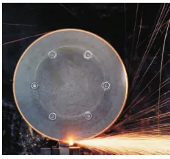
(Mikkelsen, 2014). An example of hot particles and hot spots generated during a low

speed grinding process performed by Hawksworth et al. (2004) is shown in Fig. 1.1.

The streaks of yellow/orange correspond to particles ejected from the specimen

sub-jected to the grinding, and the color of the particles is indicative of the high

tempera-tures reached. According to Hawksworth et al. (2004), for a stainless steel specimen,

the temperature at the contact spot varied from approximately 1100 to 1500 K for a

[image:35.612.261.385.528.644.2]

coefficient of friction of 0.1.

(36)

In aviation, heated particles can be generated during a lightning strike on

compos-ite aircraft structures; hot particles can be ejected from the surface that is struck due

to resistive heating. Feraboli and Miller (2009) subjected unnotched and filled-hole

CFRP (Carbon Fiber Reinforced Polymers) specimens to simulated lightning strikes

and determined that for the filled-hole specimens, the damage was confined to the

fastener and surrounding region. Figure 1.2 shows a post-mortem micrograph of a

specimen subjected to a 30 kA simulated lightning strike that destroyed the resin

and fibers on the back-face of the laminate (close to the fastener collar). Resistive

heating of the material leads to pyrolysis of the resin and fiber which can result in

an explosive release of the heated material due to gases developing from the burning

[image:36.612.235.416.318.395.2]

resin (Feraboli and Miller, 2009).

Figure 1.2: Micrograph of filled-hole specimen subjected to 30 kA simulated lightning strike, reprinted with permission from Feraboli and Miller (2009).

The motivation to study hot particle hazards stems from the possibility that hot

particles can make their way into a flammable environment and cause an unwanted

explosion that could possibly lead to damage to the surroundings, unsafe conditions,

and most importantly, loss of life. Therefore, it is important to understand the

underlying physics behind hot particle ignition, in particular, moving hot particle

ignition. As indicated by Figs. 1.1 and 1.2, the hot particles that are generated are

in motion. Additionally, the flammable mixture of interest in the present study is n

-hexane-air; n-hexane is used as a surrogate for kerosene based fuels (see Appendix A

for analysis of surrogate choice).

Hot particles come in all shapes and sizes, are made of a wide range of materials,

and can produce different flow configurations depending on whether the particle is

(37)

configurations that are possible and the resulting ignition behavior; the hot particles

are approximated as spheres.

1.2

Hot Particle Configurations

The ignition behavior of reactive mixtures in the presence of a hot particle is

depen-dent on several factors such as the particle temperature, diameter, velocity, material,

and heating method. Based on these factors, hot particles can have the following

characteristics:

1. The hot particle can be stationary or moving.

2. The particle can be heated impulsively or via a finite heating rate.

3. The hot particle size can be sub-millimeter (focus of experimental studies on

stationary hot particle ignition, see Fig. 1.12), or∼1 mm (focus of experimental

studies on moving hot particle ignition, see Fig. 1.12)

4. The hot particle can travel through a reactive mixture or travel through an

inert environment and subsequently enter a reactive mixture.

5. The hot particle material can be metallic, ceramic, glass, or a composite made

from artificial materials or cellulose fibers, i.e. reactive or inert.

These configurations do not cover non-ideal parameters such as surface temperature

inhomogeneities and particle non-sphericity.

The natural or forced convection flow over a sphere is characterized by

non-dimensional parameters such as the Froude number, Fr, Reynolds number, Re, and

Grashof number, Gr. The ignition behavior of the reactive mixture is characterized by

the Damk¨ohler number, Da, which is the ratio of the flow time scale to the chemical

time scale. The non-dimensional numbers are given in Eq. 1.1.

Fr = qU∞ gd∆_ρρ

, Re = U∞d

ν , Gr =g

∆ρ ρ

d3

ν2 , Gr =

Re Fr

2

(38)

U_∞ is the sphere or freestream velocity (sphere fixed reference frame),dis the sphere

diameter, ν and ρ are the kinematic viscosity and density of the gas, respectively,

and g is the gravitational acceleration. The Froude number represents the ratio of

inertial forces to gravitational forces, whereas the Reynolds number is the ratio of

inertial to viscous forces and the Grashof number is the ratio of buoyant to viscous

forces. Finally, the Damk¨ohler number is defined as,

Da = tflow

tchemical

, (1.2)

where

tflow ∼

d

U : forced convection

tflow ∼

δ2

T

α : diffusion.

(1.3)

In Eq. 1.3, δT is the thermal boundary layer thickness andαis the thermal diffusivity

which is written as,

α=λ/ρcp, (1.4)

whereλandcp are the thermal conductivity and specific heat of the gas, respectively.

The chemical time scale is typically defined by an ignition delay time or induction

period. During this period, the radical pool formation is increasing however depletion

of the fuel is not significant; when the pool is sufficiently large to consume the fuel,

a rapid ignition takes place (Warnatz et al., 2013).

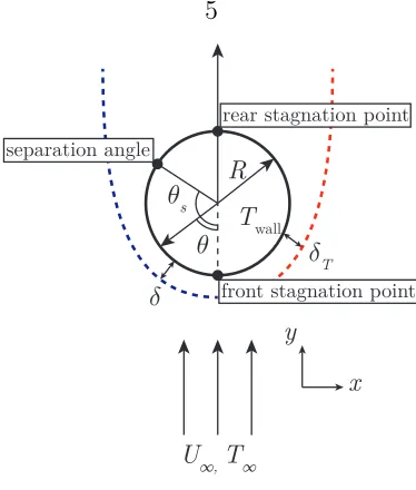
Figure 1.3 shows a schematic of laminar flow over a sphere and parameters which

are frequently mentioned in the following sections. The sphere parameters (in the

reference frame of the sphere) are based on a positive incoming freestream velocity

U_∞ and freestream temperature T_∞. The sphere has a wall temperature of Twall and

radius R. The front and rear stagnation points are labeled along with the angle at

which flow separation occurs,θs. The momentum boundary layer is delineated by the

blue dashed line on the left side of the sphere and has thickness δ that grows with

increasing angle θ. The thermal boundary layer is delineated by the red dashed line

(39)

U_∞,T_∞ y

x T_wall

R 𝜃

s

𝜃 _𝛿

T

𝛿 front stagnation point

rear stagnation point separation angle

Figure 1.3: Schematic of laminar flow with separation around a sphere.

The ratio of δ/δT varies according to the square root of the Prandtl number,

where Pr = ν/α. The ratio is less than 1 for Pr < 1 and is greater than 1 for

Pr > 1. Prandtl values as a function of gas temperature are shown in Fig. 1.4 for

n-hexane-air at various compositions. The values of Prandtl number indicate that the

thermal boundary layer should be expected to be slightly thicker (8−15%) than its

corresponding momentum boundary layer over a wide range of mixture compositions

and gas temperatures.

300 400 500 600 700 800 900 1000

T (K)

0.70 0.73 0.76 0.79 0.82 0.85 0.88

Pr

[image:39.612.229.416.54.274.2]

Φ = 0.7 Φ = 1.0 Φ = 2.0

(40)

In the present study, laminar flows with separation around a sphere are considered,

i.e. 60 < Re< 210. The corresponding Froude and Grashof numbers are ∼ 10 and

∼10₋102_{, respectively. Flows with values of Gr}_/_Re2

≥1.67 are considered to have buoyant force effects that dominate over forced convection (Chen and Mucoglu, 1977);

however, for the flows considered in the present study, Gr/Re2 << 1.

1.2.1

Stationary and Moving Hot Particles

The difference between stationary and moving hot particles is in the manner by

which the fluid surrounding the hot particle is transported, either through natural

or forced convection. Natural convection occurs when a density gradient exists in

the fluid that leads to an induced fluid velocity. Examples of streamlines in forced

convection of increasing Reynolds number flows around a sphere are shown in Fig. 1.5.

At 1 < Re < 20, the flow around the sphere is attached and axisymmetric, shown

in Fig. 1.5 (a). The onset of flow separation occurs at Re = 20 and is marked by

a change in the sign of vorticity downstream of the separation point (Clift et al.,

2005). At 20 < Re < 210, the flow has separated and is steady and axisymmetric;

the separation location moves forward along the sphere leading to wider and longer

wakes as the Reynolds number increases, shown in Fig. 1.5 (b) and (c).

(a) Re = 1 (b) Re = 150 (c) Re = 200

Figure 1.5: Streamlines surrounding sphere for increasing Re flows, from left to right; adapted from Bhattacharyya and Singh (2008) and Johnson and Patel (1999).

(41)

separated flow. The flow decelerates to zero velocity at the front of the sphere,

reaching a maximum pressure at this location; the flow then accelerates as it travels

around the sphere until it reaches a maximum velocity where the pressure is

mini-mum at θ = 90◦. Past θ = 90◦, the flow starts decelerating until it encounters an

adverse pressure gradient leading to reversal of the flow and separation. An empirical

relationship of the separation angle as a function of Reynolds number is given by

Eq. 1.5 (Clift et al., 2005), the relation is valid for 20<Re_≤400.

θs= 180−42.5

h

ln Re/20i0.483

(1.5)

At Re = 210, the flow becomes asymmetric but still maintains its steady behavior.

The onset of unsteadiness occurs at 270<Re<300 when diffusion and convection of

vorticity can no longer keep up with vorticity generation (Johnson and Patel, 1999).

U_∞

U_max

U

𝜃

separation point

P_max

P_min

𝜃

s

Figure 1.6: Evolution of the momentum boundary layer around sphere for separated flow.

The corresponding temperature contours for the flows in Fig. 1.5 are shown in

Fig. 1.7. At small Reynolds numbers the heat transfer to the fluid is primarily through

conduction in the gas, indicated by the wide thermal boundary layer in Fig. 1.7 (a).

As the Reynolds number increases, the heat transfer is dominated by convection,

indicated by the thinner and more elongated thermal boundary layers in Fig. 1.7 (b)

(42)

(a) Re = 1 (b) Re = 150 (c) Re = 200

Figure 1.7: Isotherms surrounding sphere for increasing Re flows, from left to right; adapted from Bhattacharyya and Singh (2008) and Johnson and Patel (1999).

The highest density of isotherms is at the front stagnation point of the sphere

for the cases shown in Fig. 1.7, corresponding to a large temperature gradient; the

thickness of the thermal boundary layer grows from the front stagnation point to

the rear stagnation point or forward of the rear stagnation point when the flow is

attached or separated, respectively. The large variation in the temperature within

the thermal boundary layer, due to a hot sphere and cold freestream, results in a

non-unique Reynolds number. The Reynolds number can be defined by the cold flow

gas properties or the properties of the gas immediately next to the hot sphere surface

or properties based on the average of the freestream and hot sphere temperatures,

i.e. T_∞, Twall orTfilm= (T∞+Twall)/2.

In reactive mixtures with low Reynolds numbers (Re _∼1), the shape and thickness

of the isotherms (see Fig. 1.7 (a)) suggests that ignition is possible anywhere in

the thermal boundary layer from heat release due to chemical reactions. At higher

Reynolds numbers and in separated flows, stagnation regions are created that are

likely locations for ignition when nearing the ignition threshold, i.e. the minimum

sphere surface temperature required for ignition. The ignition can be characterized

using a critical Damk¨ohler number (see Eq. 1.2), i.e. Da_≥Da∗, usually Da∗ =_O(1).

In low Reynolds number flows, corresponding to a stationary or very slow moving

(43)

boundary layer thickness and thermal diffusivity. The thermal boundary layer has

to be sufficiently thick to overcome heat losses back to the wall when there is heat

release due to chemical reactions; this also applies to higher Reynolds number flows.

In high Reynolds number separated flows, the flow time scale is governed by the

sphere diameter and freestream velocity. Fluid parcels that are entrained in the

thermal boundary layer experience a temperature increase as they travel from the

front stagnation point to the separation region; as they move past the separation

region, the fluid parcels begin to cool down as they travel within the recirculation

region (wake). For ignition to take place, a fluid parcel must ignite prior to the start

of the cooling process.

1.2.2

Particle Heating Method

A stationary particle can be impulsively heated or heated via a finite temperature

ramp. An impulsively heated particle will ignite the surrounding gas when heat has

diffused sufficiently to establish a thick enough thermal boundary layer; as noted

ear-lier, the thermal boundary layer has to be thick enough to prevent diffusive losses back

to the wall when there is heat release due to chemical reactions. When a temperature

ramp is imposed on a particle, the thermal boundary layer development is dependent

on the magnitude of the heating rate. For low heating rates, the thermal boundary

layer will develop more slowly than the thermal boundary layer of an impulsively

heated surface and the time to ignition will be longer than in the impulsively heated

case.

1.2.3

Particle Size

Increasing particle size for a fixed freestream velocity and particle temperature

re-sults in an increasing Reynolds number. This corresponds to decreasing values of θs

(according to Eq. 1.5), resulting in wider and longer wakes. Examples of isotherms

of increasing particle size are shown in Fig. 1.8. A fluid parcel that travels from the

(44)

in-creasing sphere diameters, resulting in longer flow time scales. The ignition threshold

is defined as the minimum sphere surface temperature required for ignition; in terms

of a critical Damk¨ohler number Da∗, the ignition threshold corresponds to Da_≥Da∗,

corresponding to a sphere surface temperature at which the flow time scale is

suffi-ciently large compared to the chemical time scale. The chemical time scale is usually

defined by an ignition delay time. Ignition delay times, measured with a shock tube

over a range of gas temperatures and fuels, are shown in Fig. 1.9. The logarithm of

the ignition delay time is inversely proportional to the gas temperature away from

NTC (negative temperature coefficient) region. In the NTC region (not shown in

Fig. 1.9), the ignition delay time decreases with increasing temperature.

−6−4−2 0 2 4 6

−5 0 5 10 15 20

−6−4−2 0 2 4 6

−5 0 5 10 15 20

−6−4−2 0 2 4 6

−5 0 5 10 15 20

(a) Re = 90 (b) Re = 170 (c) Re>200

Figure 1.8: Isotherms surrounding sphere for increasing particle size from left to right.1

For a fixed freestream velocity and increasing sphere diameter, the flow time scale

increases. If the ignition conditions correspond to a fixed value of critical Damk¨ohler

number, the chemical time scale must increase a corresponding amount to maintain

critical conditions. For chemical reactions in the normal (non-NTC) regime, for the

chemical time scale to increase, the gas temperature and corresponding sphere

sur-face temperature will also decrease. Therefore, the minimum ignition temperature

decreases with increasing sphere diameter; this is demonstrated by previous

experi-1_{The isotherms were obtained from 2D numerical simulations of flow past a hot sphere performed}

(45)

mental studies presented in Section 1.3. There are temperature variations within the

thermal boundary layer of the sphere, indicated by the multiple isotherms in Fig. 1.8,

making it difficult to characterize the chemical time scale using a unique gas

temper-ature. In the above analysis, the chemical time scale is defined by assuming that the

gas temperature is at the sphere surface temperature.

0.5 0.6 0.7 0.8 0.9 1.0 1.1 1.2 103_/T _(1/K)

10−2 10−1 100 101 102 103

Ignition

dela

y

time

(ms)

hydrogen-oxygen-argon:

Φ = 1,P= 3.374−3.711 atm

Φ = 0.4,P= 3.0−3.5 atm

methane-oxygen-argon

Φ = 1.0,P= 13.19−14.37 atm

Φ = 1.0,P= 35.26−37.49 atm

Φ = 0.5,P= 13.76−15.03

Φ = 2.0,P= 13.10−14.06 atm

hexane-oxygen-air

Φ = 1.0,P= 1.86−3.60 atm

Φ = 0.5,P= 1.67−1.89 atm

Figure 1.9: Ignition delay time measurements as a function of gas temperature taken from Vasu et al. (2011) (hydrogen-oxygen-argon), Davidson et al. (2012) (methane-oxygen-argon) and Davidson et al. (2010); Lam (2013) (n-hexane-oxygen-argon).

1.2.4

Inert/Reactive Environments

In the current study, the experimental setup was designed such that the particle is

heated in an inert environment, accelerated, and then injected into a reactive mixture.

Such a design ensures that ignition occurs while the particle is moving and not during

the heating phase when the particle is stationary. Due to the abrupt transition from

an inert environment to a reactive one, the inert gas has to be flushed from the

boundary layer and replaced with the reactive mixture for ignition to take place. The

flushing procedure time is on the order of the time required for a fluid parcel to travel

from the front stagnation point to the separation region or rear stagnation point;

(46)

and shorter close the edge of the momentum boundary layer where a fluid parcel is

traveling at or close to the freestream velocity (sphere fixed reference frame).

1.2.5

Particle Material/Surface

Lewis and von Elbe (1961) provided a brief summary of the effect of catalytic surfaces

on ignition. They stated that ignition occurs more readily over a noncatalytic surface

compared to a catalytic surface. A difference in the ignition behavior over catalytic

and noncatalytic surfaces exists due to radical quenching at the catalytic surface.

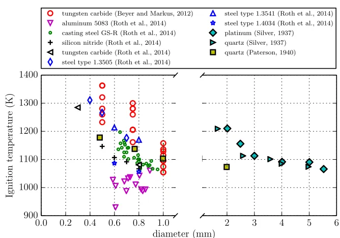
Coward and Guest (1927) heated metal strips to study the effect of surface material on

ignition of natural gas-air mixtures. They found that over a wide range of materials,

platinum yielded higher ignition temperatures compared to other materials such as

copper, gold, nickel, stainless steel, tungsten, etc. More recently, Roth et al. (2014)

quantified the effect of the surface material on the minimum ignition temperature.

Tungsten carbide surfaces resulted in higher ignition thresholds than silicon nitride

surfaces.

The hydroxyl radical (OH*) is an important radical species during an ignition

event of various reactive mixtures. The radical is created during branching chain

reactions in the thermally neutral induction period and its concentration further

increases as the temperature of the gas increases. The accumulation of radicals leads

to accelerated chemical activity, resulting in an ignition event. Suh et al. (2000)

measured the reactivity of OH* over titanium dioxide (TiO2), silicon dioxide (SiO2),

alumina (Al2O3), and gold surfaces. The reactivity was defined as the ratio of OH*

radicals that reacted on the surface to the total flux of OH* incident on the surface.

Suh et al. (2000) determined that gold was the most efficient at removal of OH*,

whereas alumina was the second most efficient and TiO2 was the least efficient. Given

that the loss of OH* depends on the surface material, ignition could potentially be

delayed for the material that showed the highest OH* reactivity: gold. Suh’s study

was performed at gas temperatures below 350 K, making it difficult to extrapolate

(47)

1.2.6

Particle Temperature Spatial and Temporal Variations

The previous subsections covering particle configurations assume that the sphere has

a homogeneous isothermal temperature distribution. This subsection provides a brief

discussion on the validity of the temperature homogeneity assumption and variation

of temperature with time after heating for the specific particle configuration used in

the present study.

Chapter 2 has a detailed description of the experimental setup used in this study

along with the experimental procedure. In summary, a stationary sphere suspended

by supports is heated for 100−300 s inside an inert environment until the desired

surface temperature is achieved, the sphere is then released and falls for 250 ms

through the inert environment before entering the reactive mixture; the sphere falls

through the reactive mixture for less than 100 ms (ignition can occur within this

time).

To ensure that the temperature is spatially uniform, heating takes place over

a much longer time scale than the characteristic time for heat conduction within

the sphere. For example, a 1.8 mm diameter sphere will reach a temperature of

approximately 1200 K in>100 s, this is a factor of 103 _{larger than the conduction time}

scale (_∼ 0.1 s) assuming material properties of titanium alloy. The heat conduction

time scale, τcond, is,

τcond=

r2

α, (1.6)

where r is the sphere radius and α is the thermal diffusivity of the solid. For a

titanium alloy sphere with a temperature of 1200 K, α = 5.5×10−6 _m2_{/s (material}

properties obtained from Figs. 2.9 and 2.10); for a r = 1 mm sphere, τcond = 0.2 s.

For an alumina sphere, α = 2×10−6 _m2_{/s and} _τ

cond = 0.5 s. The combination of

slow heating time and fast heat conduction within the sphere ensures that a sphere

has a uniform temperature distribution when it is released.

Temperature non-uniformities can also arise while the sphere is falling; the

varia-tion in edge velocity of the momentum boundary layer around the sphere results in a

(48)

2008) which can lead to temperature non-uniformities on the surface of the sphere

(Salleh et al., 2010). However, the heat transfer to the gas from the sphere occurs

over a slower time scale than heat conduction within the sphere; this is explained

using a Bio

Thermal Ignition Using Moving Hot Particles

Stephanie Alexandra Coronel

Abstract

Published Content and

Contents

List of Figures

List of Tables

Chapter 1

Hot Particle Configurations

Stationary and Moving Hot Particles

Particle Heating Method

Particle Size

Inert/Reactive Environments

Particle Material/Surface

Particle Temperature Spatial and Temporal Variations