ROBUST IDENTIFICATION FOR LINEAR-IN-THE-PARAMETERS MODELS X. Hong∗C. J. Harris∗∗ S. Chen∗∗ P. M. Sharkey∗
∗Dept of Cybernetics, University of Reading, Reading RG6 6AY, UK
∗∗Dept of Electronics and Computer Science, University of Southampton, Southampton, SO17 1BJ, UK
Abstract: In this paper new robust nonlinear model construction algorithms for a large class of linear-in-the-parameters models are introduced to enhance model robustness, including three algorithms using combined A- or D-optimality or PRESS statistic (Predicted REsidual Sum of Squares) with regularised orthogonal least squares algorithm respectively. A common characteristic of these algorithms is that the inherent computation efficiency associated with the orthogonalisation scheme in orthogonal least squares or regularised orthogonal least squares has been extended such that the new algorithms are computationally efficient. A numerical example is included to demonstrate effectiveness of the algorithms. Copyright
c
°2003 IFAC
Keywords: experimental design, structure identification, forward regression, cross validation, generalisation.
1. INTRODUCTION
A large class of nonlinear models and neural networks can be classified as a linear-in-the-parameters model (Harriset al., 2002; Wang and Mendel, 1992). The forward regression approach is an efficient model construction method (Chen
et al., 1989) for these models. Regularisation tech-niques have been incorporated into the orthogonal least squares (OLS) algorithm to produce a regu-larised orthogonal least squares (ROLS) algorithm that reduces the variance of parameter estimates (Chenet al., 1999; Orr, 1995). To produce a model with good generalisation capabilities, model se-lection criteria such as the Akaike information criterion (AIC) (Akaike, 1974) are usually incor-porated into the procedure to determinate the model construction process. Yet the use of AIC or other information based criteria, if used in forward regression, only affects the stopping point of the model selection, but does not penalise regressors
that might cause poor model performance, if this is selected at an earlier regression stage.
Parameter regularisation and robust model struc-ture selection are effective and complementary approaches for robust modelling. This paper re-views some recent advances on robust modelling techniques based on forward regression developed by the authors (Hong and Harris, 2001b; Hong and Harris, 2001a; Chen, 2002; Chenet al., 2002; Hong
et al., 2002). These algorithms aim to achieve maximum model robustness by combining param-eter regularisation and model structure selection via the direct optimisation of model robustness.
2. PRELIMINARIES
y(t) = M
X
k=1
pk(x(t))θk+ξ(t) (1)
where t = 1,2,· · ·, N, and N is the size of the estimation data set.y(t) is system output variable,
x(t) = [y(t−1),· · ·, y(t−ny), u(t−1),· · ·, u(t− nu)]T is system input vector of observables with assumed known dimension of (ny+nu).u(t) is sys-tem input variable.pk(•) is a known nonlinear ba-sis function, such as RBF, or B-spline fuzzy mem-bership functions. ξ(t) is an uncorrelated model residual sequence with zero mean and variance of
σ2. Eq.(1) can be written in the matrix form as
y=PΘ+ Ξ (2)
wherey= [y(1),· · ·, y(N)]T is the output vector.
Θ = [θ1,· · ·, θM]T is parameter vector, Ξ = [ξ(1),· · ·, ξ(N)]T is the residual vector, andP is the regression matrix
P=
p1(1) p2(1) · · · pM(1)
p1(2) p2(2) · · · pM(2) . . . .
p1(N) p2(N)· · · pM(N)
By setting a cost function of J1 = PNt=1(y(t)−
PM
k=1pk(x(t))θk)2, the least squares estimates of
Θis given by (Soderstr¨om and Stoica, 1989) ˆ
Θ= (PTP)−1PTy (3) Assume that Eq.(2) represents the data generat-ing process. IfPTPis nonsingular, then
(i)EΘˆ =Θ
(ii) cov ˆΘ=σ2(PTP)−1 (4)
where the matrix (PTP) is called the design ma-trix. It is well known that a model based on least squares estimates tends to be unsatisfac-tory for a near ill conditioned regression matrix (or design matrix). The condition number of the design matrix is given by C = maxλk
minλk, where
λk,(k = 1,· · ·, M) are the eigenvalues of the de-sign matrix. Too large a condition number of the design matrix will result in unstable parameter es-timates if a least squares algorithm is used (Harris
et al., 2002), whilst a small condition number of the design matrix leads to model robustness. Experimental design criteria of A-optimality and D-optimality (Atkinson and Donev, 1992) are introduced in Section 2.1, which provides a back-ground for Section 3.1 and Section 3.2 for two model identification algorithms.
Alternatively, parameter estimates can be de-rived based on a regularised cost function of
Jr=PNt=1(y(t)−
PM
k=1pk(x(t))θk)2+
PM
k=1γkθk2, where γk >0,k = 1,2,· · ·, M are regularisation
parameters. The regularised least squares esti-mates of Θˆris given by (Marquardt, 1970)
ˆ
Θr= (PTP+ Γ)−1PTy (5) where Γ = diag{γ1, γ2,· · ·, γM}. The concept of parameter regulasation may be incorporated into a forward orthogonal least squares algorithm as a locally regularised orthogonal least square esti-mator (see Appendix A for details), which forms the foundation for all the robust identification algorithms introduced in this paper (see Section 3).
2.1 Optimal experimental design criteria
Consider a subset model is constructed from the full model with regression matrix Pby using nθ regressors selected fromM regressors inP,nθ¿
M. Denote the resultant regression matrix Pk ∈
<N×nθ, the resultant design matrix byPT
kPk, and withλk,k= 1, ..., nθ as the eigenvalues ofPTkPk.
Definition 1: A-optimality criterion: The A-optimality design criterion, which can be applied as a model selection criterion is that which min-imises the sum of the variance of a parameter estimate vector ˆΘ = [θ1,· · ·, θnθ]
T
min{J2= tr h
cov ˆΘi=σ2
nθ
X
k=1
1
λk
} (6)
Alterntively the D-optimality design criterion can be applied as a model selection criterion that maximises the determinant of the design matrix ofPT
kPk.
Definition 2: The D-optimality criterion is that which
max{J3= det(PTkPk) = nθ
Y
k=1
λk} (7)
Maximisation of the D-optimality criterion (Atkinson and Donev, 1992) for model selection criterion inherently improves model robustness. Robust identification algorithms using the com-bined A-optimality and D-optimality with regu-larised orthogonal least squares are introduced in Section 3.1 and 3.2 respectively.
2.2 PRESS statistic
each data point in the estimation data setDN =
{x(t), y(t)}N
t=1 is sequentially set aside in turn,
a model is then estimated using the remaining (N − 1) data, and the prediction error is de-rived using only the data point that was removed. To select a model by using the delete-1 cross-validation as the model selective criterion, the model with a minimal mean squares of the pre-diction errors is selected. The prepre-diction error known as the Predicted REsidual Sums of Squares (PRESS) statistic (Myers, 1990) for linear-in-the-parameters models, can be generated without ac-tually sequentially splitting the estimation data set by using the Sherman-Morrison-Woodbury theorem (Myers, 1990). Consider a predictor that is identified based on (1), the PRESS errors
ξ(−t)(t|t−1) can be calculated using (Myers, 1990)
as
ξ(−t)(t|t−1) =y(t)−yˆ(−t)(t|t−1)
= ξ(t)
1−p(t)T[PTP]−1p(t) (8)
and the PRESS statistic is computed by
Jp=E
h
[ξ(−t)(t|t−1)]2i (9)
A robust identification algorithm using the PRESS statistic and regularised orthogonal least squares is introduced in Section 3.3.
3. ROBUST IDENTIFICATION FOR LINEAR-IN-THE-PARAMETERS MODELS
For simplicity of notation, as a function of forward regression stepk, the resultant model selection cri-teria for all the proposed algorithms are denoted asJ(k).
3.1 Combined A-optimality and ROLS
Consider the A-optimality design criterion given in Definition 1, but based on model (26) (Ap-pendix A) with orthogonal basis wk. The A-optimaility cost function that minimises the sum of the variance of the auxiliary parameter estimate vectorg= [g1,· · ·, gnθ]
T for a subset model with
nθ regressors is given by
min{JA= tr [covˆg] =σ2 nθ
X
k=1
1
κk
} (10)
Due to AΘ = g, it can be assumed that to penalize the large variance of the auxiliary param-eter vectorgwill also consequently penalize large variance of parameter vector Θ.
A composite cost function is defined as
J=J1+α1JA
= 1
N(y
Ty− nθ
X
k=1
g2kκk) +α nθ
X
k=1
1
κk (11)
where, for the sake of simplicity, α = σ2α 1, is
a positive small number. Eq.(11) can be directly incorporated into the conventional forward OLS algorithm to select the most relevantkth regressor at thekth forward regression stage, via
J(k)=J(k−1)− 1
Ng
2
kκk+
α κk
(12)
At the kth forward regression stage, a candidate regressor is selected as the kth regressor if it produces the smallest J(k) and further reduction
onJ(k−1). The selection procedure will terminate
ifJ(k)≥J(k−1)at the derived model sizenθ. This
is significant because this means that the proposed approach can automatically detect a parsimonious model size.
The above A-optimality based design model con-struction algorithm was firstly introduced by the authors in outline in (Hong and Harris, 2001b) and applied as part of the B-spline based neurofuzzy model (NeuDec) (Hong and Harris, 2001a). It was shown in (Hong and Harris, 2001b; Hong and Harris, 2001a) that the resultant models can be improved based on the reduction of model param-eter variance.
3.2 Combined D-optimality and ROLS
Consider the D-optimality design criterion given in Definition 2, but based on model (26) with orthogonal basis wk. The D-optimality design criterion that maximises the determinant of the design matrix ofWT
kWk is given by max{JD0 = det(W
T kWk) =
nθ
Y
k=1
κk}. (13)
The equivalence of (7) and (13) can be easily verified (Hong and Harris, 2002), and this implies that the selection of the a subset of Pk from P is equivalent to the selection of a subset of Wk from W, or that a better conditionedPk can be achieved via a better conditionedWk.
Construct the following cost function
JD=ψ(JD0) =−log(JD0) =
nθ
X
k=1
log[ 1
κk ](14)
Clearly the maximisation of JD0 is equivalent to
the minimisation ofψ(JD0), due to the fact that
the solution of ∂ψ(JD0) = −
1
JD0∂JD0 = 0, is
The new augumented cost function is defined as
J=J1+βJD
= 1
N(y
Ty− nθ
X
k=1
g2kκk) +β nθ
X
k=1
log[ 1
κk ] (15)
where β is a small positive number. Eq.(15) can be incorporated into the forward OLS algorithm to select the most relevant kth regressor at the
kth forward regression stage, via
J(k)=J(k−1)− 1 Ng
2
kκk+βlog[ 1
κk
] (16)
At the kth forward regression stage, a candidate regressor is selected as the kth regressor if it produces the smallest J(k) and further reduction
onJ(k−1). BecauseJ
Dis an increasing function if
κk<1, which is true for somek > K, the selection procedure will terminate if J(k) ≥ J(k−1) at the
derived model sizenθ if an properβ is set.
The complete robust identification procedure us-ing combined D-optimality and regularised or-thogonal least squares based on the forward Gram-Schmidt procedure, including optimisation of regularisation parameters, can be found (Chen
et al., 2002), in which an effective Bayesian ev-idence method (MacKay, 1992) has been intro-duced to optimise local regularisation parameters.
3.3 Combined PRESS statistic and ROLS
Alternatively the PRESS statistic of (9) that op-timises model generalation capability can be used as a robust model selective criterion. Note that (8) does not incorporate parameter regularisation. In order to combine the PRESS statistic into a model with regularisation and forward regression learn-ing algorithm, initially it is necessary to derive the PRESS error in an orthogonal weight regularised model. It can be shown (Honget al., 2002) that the PRESS error, based on the system in the orthogonalised form (given by (26)), is given
ξ(−t)(t|t−1) =y(t)−yˆ(−t)(t|t−1)
= ξ(t)
1−w(t)T[WTW+ Γ]−1w(t)
= ξ(t)
ηM(t)
(17)
where
ηM(t) = 1− M
X
i=1
w2
i(t)
κi+γi
(18)
The computational expense can be further signifi-cantly reduced by utilising the forward regression
process via a recursive formula. In the forward re-gression process, the model size is configured as a growing variablek. Consider the model construc-tion by using a subset of k regressors (k ¿ M), that is a subset selected from the full model set consisting of M initial regressors (given by (2)) to approximate the system. The PRESS errors (17)–(18) can be written, by replacing M with a variable model sizek, as
ξ(−t)(t|t−1) = ξk(t)
ηk(t) (19)
where ηk(t) = 1−Pk
i=1
w2
i(t)
κi+γi, and ξk(t) is the model residual associated with a subset model structure with k regressors.ηk(t) can be written as a recursive formula, given by
ηk(t) =ηk−1(t)−
w2
k(t)
κk+γk
(20)
This is advantageous in that, for a new model with size increased from (k−1) tok, the PRESS error coefficient ηk(t) needs only to be adjusted based on that of a model of size (k−1), with a minimal computational effort.
As in conventional forward regression (Chen et al., 1989), a Gram-Schmidt procedure is used to construct the orthogonal basis wk in a forward regression manner. At each regression step, the PRESS statistic can be formed using the algo-rithm and this is then used as a regressor selective criteria for model construction that minimises the mean square PRESS errors
J(k)=Eh[ξ(−t)(t|t−1)]2i=E[[ξk(t)]2
η2
k(t) ]
= 1
N
N
X
t=1
[ξk(t)]2
η2
k(t)
(21)
It can be analysed that due to the properties asso-ciated with the minimisation of the PRESS statis-tic, a fully automatic nonlinear predictive model contruction algorithm can be achieved (Analysis of the functionJ(k) shows that it is concave with
respect to k (Hong et al., 2002)). The complete robust identification procedure using combined PRESS statistic and regularised orthogonal least squares can be found in (Honget al., 2002).
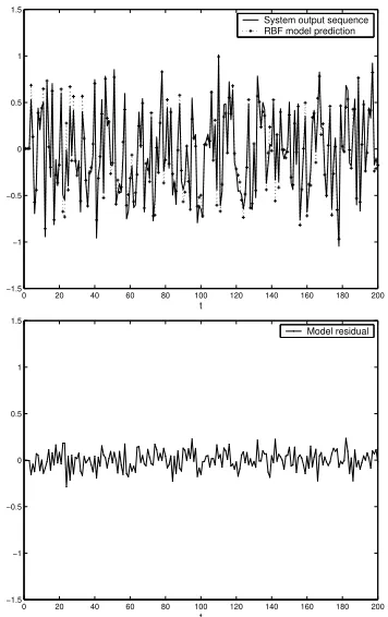
4. ILLUSTRATIVE EXAMPLE
z(t)
=z(t−1)z(t−2)z(t−3)u(t−2)[z(t−3)−1] +u(t−1) 1 +z2(t−2) +z2(t−3)
(22)
where the system input u(t) is given as a uni-formly distributed random signal in the range [−1,1]. y(x) = z(x) +ξ, in which the noise ξ ∼ N(0,0.052). 200 data points were generated. The
input vector is predetermined as a 5-input vector asx(t) = [y(t−1), y(t−2), y(t−3), u(t−1), u(t−
2)]T. The Gaussian functionφ(x, ci) = exp{−kx−
cik2/τ2}is used as basis functions to construct an RBF model, with a width τ = 1. All 200 train-ing data points are used as the candidate centre set. The proposed combined PRESS statistic and ROLS of Section 3.3 was applied for automatic model structure detection, in which the regular-isation parameter was set as γi = 10−6, ∀i. A parsimonious model structure can be detected at a derived model size when the PRESS statistic achieves at a minimum. During the forward re-gression model construction process, the PRESS statistic gradually decreases until nθ = 37, with an increment of ∆J = 1.97×10⁻⁷ > 0, such
that the model with 37 centres is automatically derived as the final model. The results of the derived RBF model with 37 centres, are shown in Fig.1. The model MSE and PRESS atnθ= 37, is 0.09952, and 0.112 respectively, demonstrating
that the model is appropriate.
0 20 40 60 80 100 120 140 160 180 200 −1.5
−1 −0.5 0 0.5 1 1.5
t
System output sequence RBF model prediction
0 20 40 60 80 100 120 140 160 180 200 −1.5
−1 −0.5 0 0.5 1 1.5
t
[image:5.595.89.267.448.731.2]Model residual
Fig. 1. Modelling results using RBF network with 37 centres.
5. CONCLUSIONS
In this paper, we have reviewed some recent ad-vances in robust nonlinear modelling techniques in the framework of forward regression, that greatly enhance the well known forward orthogonal least squares (OLS) algorithm for model selection based on various robustness objectives.
REFERENCES
Akaike, H. (1974). A new look at statistical model identification. IEEE Trans. on Auto-matic ControlAC-19, 716–723.
Atkinson, A. C. and A. N. Donev (1992). Opti-mum Experimental Designs. Clarendon Press, Oxford.
Chen, S. (2002). Locally regularization assisted orthogonal least squares regression. IEEE Trans. on Neural Networksp. Submitted. Chen, S., S. A. Billings and W. Luo (1989).
Or-thogonal least squares methods and their ap-plications to non-linear system identification.
International Journal of Control 50, 1873– 1896.
Chen, S., X. Hong and C. J. Harris (2002). Sparse kernel regression modelling using combined locally regularised orthogonal least squares and d-optimality experimental design. IEEE Trans. on Automatic Controlp. Submitted. Chen, S., Y. Wu and B. L. Luk (1999). Combined
genetic algorithm optimization and regular-ized orthogonal least squares learning for ra-dial basis function networks.IEEE Trans. on Neural Networks10, 1239–1243.
Harris, C. J., X. Hong and Q. Gan (2002). Adap-tive Modelling, Estimation and Fusion from Data: A Neurofuzzy Approach. Springer Ver-lag.
Hong, X. and C. J Harris (2001a). Neurofuzzy design and model construction of nonlin-ear dynamical processes from data. IEE Proc. - Control Theory and Applications 148(6), 530–538.
Hong, X. and C. J Harris (2001b). nonlinear model structure detection using optimum experimental design and orthogonal least squares. IEEE Transactions on Neural Net-works12(2), 435–439.
Hong, X. and C. J. Harris (2002). Nonlinear model structure design and construction using or-thogonal least squares and d-optimality de-sign.IEEE Trans. on Neural Networksp. Ac-cepted.
MacKay, D. J. C. (1992). Bayesian interpolation.
Neural Computation4(3), 415–447.
Marquardt, D. W. (1970). Generalised inverse, ridge regression, biased linear estimation and nonlinear estimation. Technometrics 12(3), 591–612.
Myers, R. H. (1990). Classical and modern re-gression with applications. 2nd Edition, PWS-KENT, Boston.
Narendra, K. S. and K. Parthasarathy (1990). Identification and control of dynamic systems using neural networks.IEEE Trans. on Neu-ral Networks1(1), 4–27.
Orr, M. J. L. (1995). Regularisation in the selec-tion of radial basis funcselec-tion centers. Neural Computation7(3), 954–975.
Soderstr¨om, T. and P. Stoica (1989).System Iden-tification. Prentice Hall.
Wang, L. X. and J. M. Mendel (1992). Fuzzy basis functions, universal approximation, and or-thogonal least squares learning.IEEE Trans. on Neural Networks3, 807–814.
APPENDIX A: LOCALLY REGULARISED ORTHOGONAL LEAST SQUARES
An orthogonal decomposition ofPis
P=WA (23)
where A = {aij} is an M × M unit upper triangular matrix and W is an N ×M matrix with orthogonal columns that satisfy
WTW=diag{κ1,· · ·, κM} (24) with
κk=wTkwk, k= 1,· · ·, M (25) so that Eq.(2) can be expressed as
y= (PA−1)(AΘ) + Ξ =Wg+ Ξ (26) where g = [g1,· · ·, gM]T is an auxiliary vector. The LROLS algorithm uses the following error criterion for parameter estimation:
Jr= ΞTΞ +gTΓg (27) Because ξ(t) is uncorrelated with past output signals, it may be shown (Chenet al., 1989) that
gk=
wT ky
wT
kwk+γk
, k= 1,· · ·, M (28)
The original model coefficient vector Θ = [θ1,
· · ·, θnθ]
T can then be calculated from AΘ = g through backsubstitution.
The ROLS procedure can use the conventional OLS procedure for model term selection which maximises model approximation capability in a forward regression manner. The principle of the method is shown below. The number of all possi-ble regressorsM can be much larger thannθ, but
nθ significant regressors can be identified using the forward OLS procedure. As the orthogonality property wT
i wj = 0 for i 6= j holds, Eq.(26) is multiplied by itself and the time average is then taken, the following equation is easily derived
1
Ny
Ty= 1
N
M
X
k=1
g2kwTkwk+ 1
NΞ
TΞ (29)
The output varianceE[y2(t)] = N1yTyconsists of two parts, N1 PM
k=1gk2wTkwk, the output variance explained by the regressors andN1ΞTΞ, the part of unexplained variance. The Error Reduction Ratio [ERR]k, which is defined as the increment towards the overall output variance E[y2(t)] due to each
regressor or input variable pk(t) divided by the overall output variance is computed through
[ERR]k =g
2
kwkTwk
yTy , k= 1,· · ·, M (30) The most relevant nθ regressors can be forward selected according to the value of the error reduc-tion ratio [ERR]k. At the kth selection, a candi-date regressor is selected as the kth basis of the subset if it produces the largest value of [ERR]k from the remaining (M −k+ 1) candidates. By setting an appropriate tolerance ρ, which can be found by trial and error or via some statistical information criterion such as Akaike’s informa-tion criterion(AIC) (Akaike, 1974) that forms a compromise between the model performance and model complexity, the variable selection is termi-nated when
1−
nθ
X
k=1
[ERR]k< ρ (31)
This procedure can automatically select a sub-set of nθ regressors to construct a parsimonious model. Equivalently, this procedure can be ex-pressed as
J(k)=J(k−1)− 1
Ng
2
kκk (32)
where J(0) =yTy. At thekth forward regression stage, a candidate regressor is selected as thekth regressor if it produces the smallestJ(k). Equation