Demand for money: a study in testing time series for long memory and nonlinearity

Demand for Money: A Study in Testing Time

Series for Long Memory and Nonlinearity

1

DEREK BOND* University of Ulster

MICHAEL J. HARRISON†

Trinity College Dublin

EDWARD J. O’BRIEN‡

European Central Bank

Abstract: This paper draws attention to the limitations of the standard unit root/cointegration approach to economic and financial modelling, and to some of the alternatives based on the idea of fractional integration, long memory models, and the random field regression approach to nonlinearity. Following brief explanations of fractional integration and random field regression, and the methods of applying them, selected techniques are applied to a demand for money dataset. Comparisons of the results from this illustrative case study are presented, and conclusions are drawn that should aid practitioners in applied time-series econometrics.

I INTRODUCTION

T

he importance of the concepts of stationarity and regime stability in economic and financial time-series modelling is well established. However, recent concerns about the interrelationship between these two concepts, and

1

1_{The authors are grateful to participants at the Irish Economics Association Conference, 2006 and} to a referee for helpful comments.

*_{[email protected].} †_{[email protected].}

‡_{[email protected]. Edward J. O’Brien, a former Government of Ireland Scholar, would like} to thank the Irish Council for the Humanities and Social Sciences for its generous funding, and to point out that the views expressed in this paper do not necessarily reflect those of the European Central Bank or its members.

the associated problems for applied work, have ensured that they remain a significant focus for research. Early studies, such as those by Bhattacharya et al. (1983), Perron (1989) and Harrison and Bond (1992),2 _{highlighted the} difficulty of distinguishing between time series generated by difference stationary processes and those generated by nonlinear but stationary processes. Since then, an increasing research emphasis has been on the problem of distinguishing between long memory and nonlinearity. The interest in long memory models has been stimulated, in particular, by a growing awareness of the limitations of the simple I(1)/I(0) framework. For example, Baillie and Bollerslev (2000) and Maynard and Phillips (2001) show how the low power of familiar unit root tests could lead to incorrect inference in the Fama (1984) regression model of the relationship between future spot and forward exchange rates, and how the empirical work could be set in a framework of fractional integration using a long memory model. Long memory models and fractional (co)integration are now popular in several other areas of the applied literature; see, for example, Gil-Alana (2003), Liu and Chou (2003), Dittmann (2004), and Masih and Masih (2004). A problem with such models is that it is not easy to distinguish them empirically from models of stationary processes with regime switching or more general nonlinearities; see, for instance, Diebold and Inoue (2001).

In the theoretical literature, two main strands of discussion have developed. The first is that of testing for structural breaks when long memory is a possibility; see Nunes et al. (1995), Krämmer and Sibbertsen (2002), and Hsu (2001). The second concerns testing for difference stationarity or fractionality against alternatives involving a structural break; see Teverosky and Taqqu (1997), Perron and Qu (2004), Dolado et al. (2005a), Dolado et al. (2005b) and Mayoral (2005). All of these studies use conventional parametric techniques for either modelling or testing. The recent development of random field regression has also provided a suite of new tests for structural breaks, nonlinearity and time-varying parameters; see, for example, Hamilton (2001) and Dahl (2002). The strength of this alternative approach is that it does not rely on any functional form being specified prior to estimation and testing.

The purpose of this paper is to compare the performance of traditional integration analysis, the fractional integration approach and random field regression-based inference, using a standard economic model and a well-known time-series dataset. The discussion is structured as follows. In Section II, the theoretical background to fractional integration and random field

regression is briefly explained. In Section III, a brief literature review is given to provide some background, and the three techniques are applied to the Johansen and Juselius (1990) money demand data. Finally, in Section IV, the results of the analysis are discussed and some practical conclusions drawn.

II THEORETICAL BACKGROUND

2.1 Fractional Integration

Traditional testing for a unit root means a choice between what Maynard and Phillips (2001) call ‘extreme alternatives’. The standard null hypothesis is that the series under consideration has a unit root, hence is only stationary after differencing. This knife-edge restriction, as Jensen (1999) puts it, appears to be far too stringent in many cases.3_{To address this, the concept of} fractional integration, introduced into time-series analysis by Granger and Joyeux (1980), has come to the fore; see the review article by Baillie (1996) for a good introduction. Put simply, in classical integration theory, a random series {y_t}_t=∞₀is said to be integrated to order d, where d is an integer, if the series has to be differenced d times to induce stationarity. In the case of fractional integration the restriction that dis an integer is relaxed. Applying a Taylor series expansion to Δd _{= (1 – L)}d _{around L = 0, where L is the lag} operator, leads to the more general differencing formula for an integrated series of order d:

1 1

Δd _y

t= yt– dyt–1+ — d(d– 1) yt–2– —d(d– 1)(d– 2)yt–3 + … (1) 2! 3!

(–1)j

+ —— d(d– 1) … (d– j + 1)y_t–j+ … j!

In the case of 0 < d< 1, it follows that not only the immediate past value of y_t, but values from previous time periods, influence the current value. Such series are said to have long memory. If 0 < d < 0.5, then {y_t} is stationary; and if 0.5 d < 1.0, the series is nonstationary.

A fundamental estimation problem is posed by the fact that Equation (1) is highly nonlinear in d. Parametric approaches to the estimation of d are

3_{The long-run behaviour of the random variable y}

t in the simple AR(1) model with drift,

computationally intensive as they often involve the estimation of a covariance matrix and so face issues of robustness in large samples. In the case of maximum likelihood, estimation also requires the stationarity restriction 0 <d< 0.5. Nonparametric approaches have been suggested, utilising the frequency domain. These are usually robust to nonstationarity but suffer from small sample bias.

A few econometric packages provide software to handle the estimation of the fractional integration parameter, d. Initially, the software tended to be for nonparametric methods, such as the log-periodogram regression method (GPH) introduced by Geweke and Porter-Hudak (1983). Now, a wider range of methods is available. For example, in the OX-based ARFIMA package of Doornik and Ooms (1999), both parametric and nonparametric methods are provided. Exact maximum likelihood estimation (EML) is implemented using the computationally efficient approach suggested by Sowell (1992). The An and Bloomfield (1993) modified profile likelihood estimator (MPL) is also available. Both the EML and MPL methods are only applicable when d< 0.5, so the package also provides an approximate maximum likelihood estimator based on minimising the sum of squared naïve residuals, which was developed by Beran (1995). Doornik and Ooms (1999) refer to this as nonlinear least squares (NLS). To complement these parametric estimators, the ARFIMA package provides two standard nonparametric methods. The first is GPH and the second is the Gaussian semiparametric method (GSP) discussed in Robinson and Henry (1998). Other methods that are gaining popularity include the modified log-periodogram estimator (MLP) of Kim and Phillips (1999) and the generalised minimum distance estimator (GMD) of Mayoral (2003).

An interesting group of tests, based on the ADF test, has been introduced by Dolado et al. (2002) and this has been further developed in Dolado et al. (2005a, 2005b) and Mayoral (2005). The latter two papers consider the important case of testing for long memory against structural breaks and use a modified ADF framework. This framework considers the t-test statistic on the ordinary least squares (OLS) estimator of φin the generalised ADF equation

p

Δd0_y

t= φΔd1 yt–1+

冱

ζiΔyt–i+ εt. (2) i=1

For testing purposes d₀is set equal to 1. Dolado et al. (2002) show that if 0.5 d₁ < 1, then the t-statistic for the null hypothesis H₀:φ = 0 has an asymptotic standard normal distribution; and if 0 d₁ < 0.5, the t-statistic follows a nonstandard distribution of fractional Brownian motion. In practice, d₁ is unknown so a consistent estimator of it has to be used. Dolado et al. (2002) prove that provided a T–1–2 _{consistent estimator of d}

1 is used, the

t-statistic has a normal distribution asymptotically for 0 d₁< 1.

2.2 Random Field Regression

The paper by Hamilton (2001) introduced the idea of using random field models to estimate nonlinear economic relationships. A by-product of Hamilton’s approach was a new test for nonlinearity based on the Lagrange multiplier principle.

2.2.1 Estimation

The basic random field regression model is of the form

y_t= μ(x_t)+ ε_i, ε_t⬃N(0, σ2_{), t= 1, 2, … T, (3)}

where x_tis a k-vector of observations on the explanatory variables at time t, and the functional form of the conditional mean, μ(x_t), is unknown, being assumed to depend on the outcome of a Gaussian random field. In his paper, Hamilton suggests representing μ(x_t) as consisting of a deterministic linear component and a stochastic, unobservable nonlinear component, both of which contain unknown parameters that need to be estimated, i.e.,

μ(x_t) = α₀+ αα'x_t+ λm(x-_t), (4)

x-_t= g_°x_t, (5)

is the function m(x-_t) that is specifically referred to as the random field, and there are several possible specifications for this. Hamilton (2001) showed how, under fairly general misspecification, it is possible to obtain a consistent estimator of the conditional mean under fairly weak conditions. In addition, Dahl (2002), Dahl and González-Rivera (2003) and Dahl and Hylleberg (2004) show that the random field approach has relatively better small sample fitting and forecasting abilities than a wide range of parametric and nonparametric alternatives.

Viewing m(x-_t) as a realisation of a simple Gaussian random field has the advantage that it can be fully described by its first two moments:

E(m(x-_t)) = 0, (6)

E(m(x-_t)m(x-_s)) = H(d_L* (x-_t, x-_s)), (7)

where d_L* (x-_t, x-_s)僆ᑬ₊ is a distance measure. An additional simplifying assumption is that the realisation of the functional form occurs prior to, and therefore independently of, all observations on x_t and ε_t. Hamilton (2001) chooses a generalised version of the so-called spherical covariance function used in geostatistical literature:

G_k–1(h_ts, 1)

H_k(h_ts) = ————— hG_k–1(0, 1) ts1, (8) 0 h_ts> 1,

G_k (h_ts, r) =

冮

r hts

冢

r

2_{– z}2

冣

k –₂

dz, (9)

h_ts= d_L* (x-_t, x-_s), t, s= 1, 2, … T, (10)

where H_k(h_ts) is the t-sth_{entry in the TTcovariance matrix H.}

As m(x-_t) is not observable, the approach is to draw likelihood-based inference about the unknown parameters of the model, say, ϕϕ= {α₀,αα,λ,g,σ}, from the observed realisations of y_t and x_t. The likelihood function can be derived by re-writing Equations (3) and (4) for all observations, in an obvious notation, as

y= Xββ+ νν, (11)

νν⬃N(0, λ2_{H+ σ}2_I

T), (12)

where

νν''= [λm(x-₁) + ε₁,λm(x-₂) + ε₂,λm(x-₃) + ε₃, …, λm(x-_T) + ε_T]. (13)

Thus maximising the likelihood function to obtain an estimate of ϕϕ is a

generalised least squares problem. Letting ζ= λ–

σand W(X;g;ζ) = ζ2 H+ σ2IT, the profile log-likelihood function associated with the least squares problem can be obtained as

T T 1 T

η(y,X,g;ζ) = – — ln(2π) – — ln σ2 _{(g; ζ) – – ln |W(X;g;ζ)| – —, (14)} 2 2 2 2

while

ββ⬃(g; ζ) = [X''W(X;g;ζ)–1X]–1[X''W(X;g;ζ)–1y], (15)

1

σ ⬃2

(g; ζ) = — [y – Xββ(g;ζ)]'' W(X;g;ζ)–1 [y – Xββ(g;ζ)]. (16) T

The profile log-likelihood function is maximised with respect to (g;ζ) using standard maximisation algorithms, though as Bond et al. (2005) point out, care needs to be taken when maximising the log-likelihood due to computational pitfalls. Once estimates for g and ζ have been obtained, Equations (15) and (16) can be used to obtain estimates of ββ and σ.

2.2.2 Testing

The model proposed by Hamilton suggests that a simple approach to checking for nonlinearity is to test the null hypothesis H0:λ2= 0 (or λ = 0), using the Lagrange multiplier principle. Hamilton (2001) derived the appropriate score vector of first derivatives and the associated information matrix. Details of the procedure are given by Hamilton (2001), and summarised in Bond et al. (2005), but the main steps of the test are presented here for convenience.

2

● Set g_i= —–— ,where s_i2 is the variance of explanatory variable x_i, excluding

冪苴苴ks_i2

the constant term whose variance is zero.

1

● Calculate theTTmatrix, H, whose typical element is H_k

冢

– ||x-_t, x-_s,||

冣

, i.e., 2

● Use OLS to estimate the standard linear regression y= Xββ + εεand obtain the usual residuals, εεˆˆ , and standard error of estimate, σˆ2_{= (T – k – 1)}–1_εεˆˆ''_{εεˆˆ .}

● Finally, compute the statistic

[εεˆˆ''Hεεˆˆ –σˆ2_tr(MH)]2

κ2_{= ———————–———————————, (17)}

σˆ4_{{2tr([MHM–(T – k – 1)}–1_Mtr(MH)]2_)}

where M = I_T– X(X''X)–1_{X''is the familiar symmetric idempotent matrix.} As κ2_⬃A_χ

12 under the null hypothesis, linearity (λ2= 0) would be rejected if

κ2 _{exceeded the critical value, χ}2

1,α, for the chosen level of significance, α. Otherwise the null of linearity would not be rejected. For example, at the 5 per cent significance level, the null would be rejected if κ2_{> 3.84. In this case the} alternative nonlinear specification given by (4) would be preferred. The identification of a specific form of nonlinearity is aided by the estimate of the conditional expectation μ(x_t) and, specifically, the ζ⬃and g⬃. The matter is explained in Hamilton (2001, Section 5) and illustrated in the three examples in his Section 7.

III AN EMPIRICAL CASE STUDY

To investigate the application of both the new long memory tests and the random field approach, a standard applied economics problem, namely, the estimation of demand for money functions, is considered in this section. The demand for money is one of the most debated issues in economics. A simple monetarist view is that money demand is a stable function of national income, whereas Keynesian claims imply that it is not. A stable money demand equation may be considered very important for conducting monetary policy but there are several reasons for suspecting instability, including changes in the monetary regime and approaches to monetary policy and, in Europe, the creation of the European Monetary System and Euro zone. Indeed, there has been much research into the nature and stability of the demand for money in many countries, and some of the more recent literature is reviewed briefly in the next subsection.

3.1Background

Ericsson et al. (1998), Fiess and McDonald (2001) and Mark and Sul (2003).4 However, concerns have been expressed about the use of this methodology in the presence of structural breaks; see, for example, Campos et al. (1996). Therefore some modern research has employed recently developed econometric methods to analyse possible instability and nonlinearities; see, especially, the papers by Wolters et al. (1998) and Lütkepohl et al. (1999), which examine the impact of unification on the German demand for money, using tests based on the smooth transition regression (STR) models described in Teräsvirta (1998). Choi and Saikkonen (2004) also make use of this recent STR model. There seems to be no previous study of money demand that has used the factional integration and random field regression approaches used in the present paper.

3.2Data

The well-known datasets provided by Johansen and Juselius (1990) for Denmark and Finland are used for our case study. These contain, for Denmark, quarterly observations on the M2 measure of money demand, gross domestic product, the inflation rate, the deposit interest rate and the bond rate for the period 1974 to 1987, inclusive; and for Finland, quarterly observations on the M1 measure of money, real national income, the inflation rate and the marginal interest rate of the Bank of Finland for the period 1958 to 1984, inclusive. Thus there are 55 quarterly observations available for Denmark and 106 for Finland. The logarithms of all variables, except the bond and interest rates, are used. Plots of the Danish and Finnish log money demand series against time are given in Figures B.1 and B.2, respectively.5

3.3Methodology

The standard I(1)/I(0) analysis is conducted first, in Subsection 3.4.1. The univariate analysis of the series, using the augmented Dickey-Fuller (ADF) testing strategy proposed by Dolado et al. (1990) is implemented to determine whether the individual series are trend stationary or difference stationary.6 The unit root tests due to Kwiatkowski et al. (1992) (KPSS), Elliott et al. (1996) (ERS), and Ng and Perron (2001) (NP) are also employed. Both the Engle and Granger (1987) error correction (ECM) and Johansen (1988) vector

4_{An early study on the estimation and stability of the demand for money function in Ireland is} that by Browne and O’Connell (1977), which pre-dates cointegration methodology.

5_{Figures with numbers preceded by B are in the online appendix, Web-Appendix B. The full} dataset is available from the website www.math.ku.dk/~sjo/.

autoregression (VAR) approaches are used to investigate the possibility of cointegration, with the augmented Engle-Granger (AEG) test, the cointegrat-ing regression Durbin-Watson (CRDW) test of Sargan and Bhargava (1983), and the ECM test due to Banerjee et al. (1986) being used in the former case. The p-values from MacKinnon (1996), MacKinnon et al. (1999), Ericsson and MacKinnon (2002), and standard normal tables are used, as appropriate. The effect of applying Johansen’s (2002) small sample correction is also examined.

The long memory and fractional integration analysis is undertaken in Subsection 3.4.2. Only univariate analysis is attempted, due to the complexity of fractional cointegration models. In particular, it seems unlikely that the series in either of the two cases considered all have the same level of fractional integration. The ‘over differenced’ ARFIMA model, using Δy_trather than y_t, is estimated, as recommended by Smith et al. (1997), to avoid the problems associated with drift. Four estimates of d are calculated using the Doornik and Ooms (1999) ARFIMA package, namely, the EML, NLS, GPH and GSP estimates. The fact that the first of these requires d< 0.5 is another reason for using the ‘over-differenced’ model.7 _{The estimates of d are then used in the} fractional Dickey-Fuller (FDF) and fractional augmented Dickey-Fuller (FADF) tests, with the Schwarz information criterion (SIC) being used as the basis for the choice of the lag length for the test.

In Subsection 3.4.3, the random field regression approach is applied to the two cases, using the GAUSS code provided by Hamilton at his website, http://weber.ucsd.edu/~jhamilto/. Subsection 3.4.4 contains comments on the results produced and on the alternative models they suggest.

3.4Demand for Money in Denmark and Finland 3.4.1 Standard Analysis

Following Johansen and Juselius (1990), a simple demand for money function can be specified for Denmark and Finland as

m_t= α+ β₁y_t+ β₂p_t+ β₃i_t+ β₄b_t+ ε_t, (19)

where m_tis the logarithm of a measure of money demand, y_tis the logarithm of real income, p_tis the logarithm of the inflation rate, i_tis the deposit interest rate and b_tis the bond rate at time t. For Finland, β₄ is assumed to be zero as no bond rate data are available.8

7_{The MPL estimate is not obtained as there are no ‘nuisance’ parameters in the model being} estimated.

Tables A.1 and A.2 give the results of the Dolado et al. (1990) unit root testing strategy for the Danish and Finnish variables, respectively.9 _For Denmark, all of the data series appear to be clearly I(1). However, for the Finnish data, only the m_tand y_tvariables seem to be I(1), though the inference is marginal for y_t. In the case of Finland’s m_tvariable, the constant in the ADF test is only marginally insignificant, but if it is treated as significant, the ADF test still supports the null of a unit root, with a test statistic of –0.760 and an associated p-value of 0.826. By contrast, the unit root null is rejected decisively for Finland’s p_t and i_tseries. It is noteworthy, though, that if, for these last two variables, the Akaike information criterion (AIC) is used instead of the SIC, the choice of lag lengths for the ADF tests, and the test results, are different: the suggestion then is that, like m_t and y_t, the Finnish price and interest rate variables are also I(1).

To investigate further, the KPSS, ERS and NP alternative unit root tests are conducted. While the latter two tests have as their null hypothesis that the series has a unit root, the first has the null that the series is stationary and the alternative hypothesis that it has a unit root. For the Danish data the additional tests broadly confirm the findings of Table A.1. In only a few cases does the KPSS test fail to reject the null hypothesis of stationarity. One case is that of the money demand variable, m_t, when Parzen kernel estimation is used and no trend is specified. The other is that of the income variable, y_t, when a trend is allowed for in the specification.10 _{For the Finnish data the} results are less clear. For all variables, the NP test, which may have better power than standard I(1)/I(0) tests, tends to reject the null hypothesis of a unit root. This is often supported by the KPSS and ERS tests.11

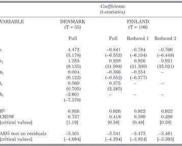
On the assumption that the variables are I(1), which seems to be a far safer assumption to make for Denmark than for Finland, the Engle-Granger two-step approach to cointegration gives the estimated levels models, and associated AEG and CRDW test results for the OLS residuals, presented in Table 1. Using the 5 per cent significance level, there is little evidence for both countries that a cointegrating money demand relationship might exist. Only in the case of Finland, when p_tand i_tare ignored in view of the fact that they seem to be I(0) using the Dolado et al. (1990) procedure and the supplementary unit root checks, is cointegration of m_t and y_t suggested by the AEG and CRDW tests, but even then only marginally.

9_{Tables with numbers preceded by A are presented in the online appendix, Web-Appendix A.} 10_{In this latter case, the result holds for any of the spectral estimation methods, but not for the} moment estimators.

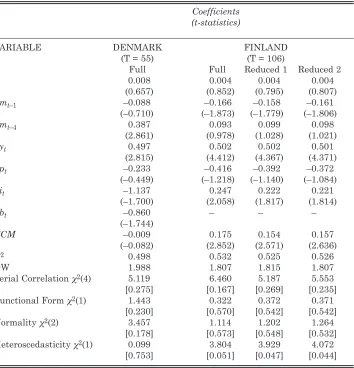
The estimates of parsimonious error correction models, using the lag of the residuals from the levels regression models as the error correction terms, are given in Table 2. The models are statistically acceptable in the sense that they are supported by a range of misspecification diagnostics. Only in the case of the equations for Finland is there a marginal suggestion of heteroscedasticity. However, with R2_{values around 0.5, the fits are quite poor and there is a high} incidence of insignificance of the estimated coefficients. In particular, the coefficients on the error correction terms are highly insignificant, with three of the four being perversely signed; and the ECM test decisively rejects cointegration in all cases. Even in the one case for Finland in which the AEG and CRDW tests suggest the possibility of cointegration, the ECM test rejection is unambiguous.

[image:12.499.75.433.97.384.2]

The Danish data have been used extensively by Johansen and it is clear from his results that the argument that there is a cointegrating money demand relationship depends largely on the VAR specification and the test

Table 1: Engle-Granger Levels Models

Coefficients (t-statistics)

VARIABLE DENMARK FINLAND

(T = 55) (T = 106)

Full Full Reduced 1 Reduced 2

c 4.472 –0.841 –0.784 –0.766

(5.178) (–6.552) (–6.104) (–6.448)

y_t 1.283 0.928 0.926 0.921

(9.135) (31.988) (31.300) (35.021)

p_t 0.004 –0.366 –0.254 –

(0.122) (–0.552) (–0.377)

i_t 0.569 0.375 – –

(0.705) (2.285)

b_t –2.601 – – –

(–7.370)

R2 _{0.926 0.926 0.922 0.922}

CRDW 0.737 0.418 0.399 0.398

[critical values] [1.19] [0.58] [0.48] [0.38]

AEG test on residuals –3.301 –3.541 –3.473 –3.461

[critical values] [–4.694] [–4.204] [–3.824] [–3.395]

[image:13.499.72.426.98.466.2]

statistic used; see Johansen (1988), Johansen and Juselius (1990) and Johansen (2002). Table A.3 gives a summary of the results that can be obtained for Denmark using Johansen’s approach and a VAR lag length of one, as suggested by the SIC and the adjusted likelihood-ratio test.12_{As can be} seen, a range of specifications concerning intercepts and trends is examined for variants of the model with and without seasonal dummy variables.

Table 2:Error Correction Models

Coefficients (t-statistics)

VARIABLE DENMARK FINLAND

(T = 55) (T = 106)

Full Full Reduced 1 Reduced 2

c 0.008 0.004 0.004 0.004

(0.657) (0.852) (0.795) (0.807)

Δm_t–1 –0.088 –0.166 –0.158 –0.161

(–0.710) (–1.873) (–1.779) (–1.806)

Δm_t–4 0.387 0.093 0.099 0.098

(2.861) (0.978) (1.028) (1.021)

Δy_t 0.497 0.502 0.502 0.501

(2.815) (4.412) (4.367) (4.371)

Δp_t –0.233 –0.416 –0.392 –0.372

(–0.449) (–1.218) (–1.140) (–1.084)

Δi_t –1.137 0.247 0.222 0.221

(–1.700) (2.058) (1.817) (1.814)

Δb_t –0.860 – – –

(–1.744)

ECM –0.009 0.175 0.154 0.157

(–0.082) (2.852) (2.571) (2.636)

R2 _{0.498 0.532 0.525 0.526}

DW 1.988 1.807 1.815 1.807

Serial Correlation χ2_{(4) 5.119 6.460 5.187 5.553}

[0.275] [0.167] [0.269] [0.235]

Functional Form χ2_{(1) 1.443 0.322 0.372 0.371}

[0.230] [0.570] [0.542] [0.542]

Normality χ2_{(2) 3.457 1.114 1.202 1.264}

[0.178] [0.573] [0.548] [0.532]

Heteroscedasticity χ2_{(1) 0.099 3.804 3.929 4.072}

[0.753] [0.051] [0.047] [0.044]

Note:For diagnostics, p-values in square brackets.

Examination of the various VAR estimates suggests that the specification with unrestricted intercept and trend is the most appropriate. Moreover, given that the data used are quarterly, the variant with seasonal dummies is also preferred. There is variability in the suggested number of cointegrating relationships across the range of specifications used, and between the trace test and the maximal eigenvalue test used to ascertain this number. The surprise is that despite the results from the static cointegrating regressions and error correction models, which overwhelmingly point to no cointegration, all of the results in Table A.3, except one, suggest at least one cointegrating vector. In the case of the preferred specification, the suggestion is of one cointegrating relationship, in contrast to the outcome produced by the Engle-Granger approach.

For the Finnish data, the summary results of the Johansen procedure on the full model are given in Table A.4. There is similar variability in the number of cointegrating relationships suggested for the different specifications and tests to that noted for Denmark, though it is not quite as marked. The preferred specification is again that with unrestricted intercept, unrestricted trend and seasonal dummies, for which case the number of cointegrating relationships indicated is two, again in stark contrast to the earlier indications of no cointegration. Accordingly, two alternative reduced models for Finland are also investigated: one taking p_tto be I(0) in the VAR analysis, and the other treating both p_tand i_tas I(0). The summary results for these cases are given in Table A.5 and Table A.6, respectively. Table A.5 contains consistent indications of a single cointegrating vector across all VAR specifications and tests, though once again this finding contradicts the indications from the AEG, CRDW and ECM tests. Slight variability in the results for different specifications and tests is seen in Table A.6, but in this case no cointegration is suggested for the preferred specification. This finding conflicts with the corresponding AEG and CRDW results, which indicate a possibility of cointegration, but it is in agreement with the ECM test result.

indicating one cointegrating relationship. The correction factors are close to unity for the Finland cases, probably due to the larger sample size. Even so, the outcome for the full Finnish model is similar to that for Denmark, the modified trace test indicating the reduced number of one cointegrating relationship, while the maximum eigenvalue test indicates two. However, the correction has no effect in the cases of the two reduced models.13 _The conclusion suggested by the modified Johansen procedure remains that the number of cointegrating vectors is one and zero for the first and second reduced Finnish models, respectively.

It can be seen from these various results that the traditional analysis is somewhat confusing. Examination of the Danish data seems to suggest that all variables are I(1) and, using the Engle-Granger two-step procedure, that cointegration does not hold and error correction models are not appropriate. Yet, using the original Johansen VAR approach, there are strong indications of cointegration, which are only challenged if a bias corrected trace test is undertaken. The Finnish data give rise to some similar findings, although in contrast to the Danish case, unit root tests suggest that some of the series are possibly not I(1). When allowance is made for this possibility, the Engle-Granger approach marginally supports cointegration, but the Johansen technique gives contrary results, whether or not a modified trace test is used, indicating that there is no cointegration.

3.4.2 Fractional Integration

Having raised concerns over the standard I(1)/I(0) analysis, the next step is to consider the possibility of fractional integration. Table A.11 gives the results of the fractional analysis for the Danish data. For each variable, a range of estimates of dis provided, as well as the results of the FDF and FADF tests. The corresponding results for the Finnish data are given in Table A.12. It can be seen from the results that there is little evidence in support of the Danish data being anything other than I(1), which accords with the findings of the previous standard analysis. It is possible, if just the parametric estimators of d are considered, to argue that the Danish b_t variable is fractionally integrated, whereas for the Finnish data it would appear that three of the four variables are fractionally integrated, namely, m_t, p_tand i_t. It will be recalled that unit root tests decisively rejected the unit root null for the latter two variables. The results for Finland’s y_tvariable also give indications that it is fractionally integrated, but the FADF result in this case has the

wrong logical sign. Overall, the investigation of fractional integration suggests that the Finnish data series are not generated by I(1) processes but that the Danish data are.

3.4.3 The Hamilton Approach

In light of the possibility that the emerging difficulties may be related to parameter instability, or some other type of nonlinearity, of what may be stationary data generating processes, simple recursive residual plots for the Danish and Finnish versions of model (19) are produced; these are depicted in figures B.3 and B.4, respectively. Guided by these graphs, simple Chow breakpoint tests for the Danish and Finnish models are implemented and the results of these are given in Table A.13. Finally, Hamilton’s random field approach is used to explore the likely form of the two models, and this leads to some interesting results. The graphs and Chow tests provide strong initial evidence for structural instability in both models. Hamilton’s LM test statistics for nonlinearity for the Danish and Finnish models are 15.338 and 123.810, respectively, which are significantly greater than the 5 per cent critical χ₁2_{value of 3.84, again suggesting that the models should not be simple} linear models. Detailed results from the Hamilton procedure are given in Table 3.

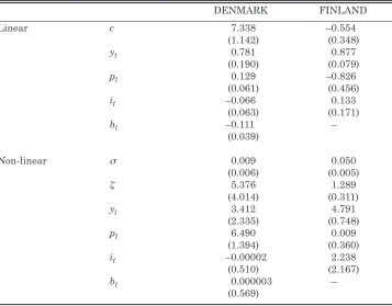
Given the earlier findings, the Hamilton results from the Danish data are rather disappointing, in so much as both σ and ζ estimates are not statistically significant on the basis of an asymptotic t-test. It could be argued, along the lines of Dahl and González-Rivera (2003), that this is due to nuisance parameter problems, given that under the null of linearity, the g_iparameters are unidentified. If the statistical insignificance of σ⬃ and ζ⬃ is ignored, the significant coefficient of p_tin the linear and the nonlinear components of the Danish model strongly suggests that this inflation variable is the prime source of any parameter instability.

In the case of Finland, the results in Table 3 indicate that both σ⬃and ζ⬃are statistically significant, in agreement with the implied value of λ in the LM test, suggesting that there is significant nonlinearity in the money demand relationship. In the Finnish case, it is the income variable, y_t, that proves significant in both the linear and nonlinear parts of the model and, therefore, needs to be investigated further.

3.4.4 Comments on the Hamilton Results

[image:17.499.68.425.99.378.2]

EEC in the mid-1970s. This arrangement continued in the form of the Exchange Rate Mechanism within the European Monetary System from 1979 and, as the Deutschmark was effectively the nominal anchor in the currency co-operation, this put severe pressure on Danish competitiveness because of a markedly higher inflation rate in Denmark compared to Germany. The result was a series of four discrete devaluations from 1979 to 1982, which served to improve Denmark’s trade balance somewhat but did little to compensate for the increasing costs of old loans at a time when international real interest rates were already high.14 _{Indeed, the Danish devaluation strategy} exacerbated this problem. Given this background, it is noteworthy that the Hamilton analysis puts inflation at the root of the nonlinearity that is detected. This finding is also in line with some of the results in Johansen and Juselius (1990), though they provide little interpretation of their results.

Table 3: Hamilton Analysis Estimates

DENMARK FINLAND

Linear c 7.338 –0.554

(1.142) (0.348)

y_t 0.781 0.877

(0.190) (0.079)

p_t 0.129 –0.826

(0.061) (0.456)

i_t –0.066 0.133

(0.063) (0.171)

b_t –0.111 –

(0.039)

Non-linear σ 0.009 0.050

(0.006) (0.005)

ζ 5.376 1.289

(4.014) (0.311)

y_t 3.412 4.791

(2.335) (0.748)

p_t 6.490 0.009

(1.394) (0.360)

i_t –0.00002 2.238

(0.510) (2.167)

b_t 0.000003 –

(0.569)

Note:Standard errors in parentheses.

In Finland, the development of the economy was rather uneven during the sample period. The gap between Finnish GDP per capita and that of the EU15 had been widening during the 1950s, which led to a devaluation and an easing of foreign trade regulations in 1957. The gap was stabilised, but convergence towards the EU15 GDP per capita level was only achieved following a further devaluation in 1967.15_{Indeed, despite the difficulties caused by the oil crisis} in the 1970s, Finland’s GDP per capita exceeded that of the EU15 by the early 1980s, i.e., the end of our sample period. Given the policy focus on GDP per capita, it may be no coincidence that the variable suggested as the source of the nonlinearity detected in the Finnish case is income. However, as Johansen has pointed out, the interpretation of the findings for the Finnish data poses particular problems.

It is not the intention here to pursue in detail the issue of re-specification of the demand for money functions for Denmark and Finland. As has been made clear, this empirical study is simply intended to illustrate the application of new econometric approaches and provide a basis of comparison between the findings from these and the results obtained from standard methods. However, two tentative possibilities are examined briefly.

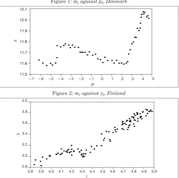
The cross plots of m_t against p_t for Denmark, and of m_t against y_t for Finland, given in Figures 1 and 2, respectively, hint at the possibility of a piecewise linear regression being an adequate model for the money demand relationships.16_{In the case of Denmark, such a model is estimated by OLS to} be

m_t= 6.66 + 0.93y_t+ 0.54p_t– 0.65(p_t– p₁)D_1t+ 1.25(p_t– p₂)D_2t

(0.67) (0.11) (0.14) (0.16) (0.17)

+ 0.61i_t– 1.48b_t+ ε_t, (20)

(0.58) (0.31)

where the numbers in parentheses are standard errors and ε_t is the OLS residual at time t. For Finland, the estimated piecewise model is

m_t= 1.77 + 0.31i_t– 0.32p_t+ 0.30y_t+ 0.88(y_t– y₁)D_1t+ ε_t. (21) (0.27) (0.12) (0.46) (0.06) (0.09)

In both cases the extra terms are highly significant. Furthermore, the R2 values are about 0.95 for both equations and the misspecification diagnostics for nonnormality, heteroscedasticity and functional form are also satisfactory.

[image:19.499.67.427.233.591.2]

However, there are significant indications of first-order autocorrelation from the Durbin-Watson test, as well as fourth-order autocorrelation from the relevant Lagrange multiplier test.17 _{Moreover, when the Hamilton test for} nonlinearity is applied to these revised equations, the sample values of the LM statistics for the Danish and Finnish models are 42.987 and 18.354, respectively, which are still higher than the critical χ₁2 value of 3.84. This finding contradicts the indications provided by the first test for nonlinearity (RESET), which suggests that functional forms (20) and (21) are adequate. Though the substantial fall in the value of the Hamilton test statistic for the Finnish data is encouraging, Hamilton’s method suggests that both models are still not appropriately specified.

Figure 1: m_tagainst p_t, Denmark

12.1

12.0

11.9

11.8

11.7

11.6

11.5

p

–.7 –.6 –.5 –.4 –.3 –.2 –.1 .0 .1 .2 .3 .4 .5

m

Figure 2: m_tagainst y_t, Finland

4.0

3.8

3.6

3.4

3.2

3.0

2.8

3.8 3.9 4.0 4.1 4.2 4.3 4.4 4.5 4.6 4.7 4.8 4.9 5.0

m

y

Alternatively, the use of a smooth transition regression (STR) model to handle the nonlinearity in the case of Finland produced generally mixed results, despite the success of such models in the German studies by Wolters et al. (1998) and Lütkepohl et al. (1999) referred to in Subsection 3.1. However, guided by results of tests of linearity against the STR described by Teräsvirta (2004, p. 222), a specification involving just y_tas the explanatory variable gave a considerably better outcome. In this case, Hamilton’s test yielded a κ2 _value of 2.67, suggesting that the nonlinearity is adequately modelled by a smooth transition regression.18

IV SUMMARY AND CONCLUSIONS

This paper has drawn attention to some of the pitfalls involved in using the conventional I(1)/I(0) framework for economic and financial modelling of time-series data, an approach involving well-known unit root tests and the cointegration testing and modelling procedures of Engle and Granger (1987), and Johansen (1988), that has been applied widely by economists during the last decade or so. The practical difficulties of untangling the issues of stationarity, fractional integration, nonlinearity, and parameter instability have been highlighted. In addition, the recent research directed at resolving these problems and providing alternative, or at least complementary, approaches to modelling has been discussed. Brief accounts have been given of the theory underlying fractional integration and long memory models, and of the estimation and testing methods in the random field regression approach proposed by Hamilton (2001). Guidance has also been provided on the several methods of estimating and testing the order of fractional integration and the software necessary for the implementation of these and the Hamilton method. A key element in the paper has been the presentation of a case study to illustrate the application of these newer techniques and contrast their findings with those of the standard cointegration modelling approach. The study used the data previously analysed by Johansen and Juselius (1990) in connection with demand for money functions in Denmark and Finland. The results obtained exemplify the problems with the standard approach and the alternative conclusions that might be reached by using different techniques. The findings, using the standard approach, are as follows.

● Though ADF tests, implemented using the Dolado et al. (1990) procedure, appear to suggest unit roots for most variables, they are sensitive to the specification of the test equation and the information criterion used to choose lag length in the case of some variables, especially for Finland.

● When the matter of unit roots was explored further, using the ERS, KPSS and NP tests, unit roots for the Danish variables tended to be confirmed but not for the Finnish variables.

● Proceeding on the assumption that all variables are I(1), the Engle-Granger two-step procedure does not support cointegration in general, a result that is confirmed by ECM tests conducted in an error-correction framework for the money demand relationship for each country. However, the Engle-Granger approach does suggest cointegration for the version of the Finland model that treats two of the variables, p_tand i_t, as I(0).

● Using the Johansen approach without its small sample bias-correction factor, there is considerably stronger evidence of cointegration in the case of Denmark, though the number of cointegrating vectors suggested varies, depending on the VAR specification chosen. For the preferred VAR specification, one cointegrating vector is suggested for Denmark. The picture that emerges for Finland is similar, although for the version of the model that treats the p_t and i_t variables as I(0), the Johansen method suggests no cointegration, contradicting the finding of the Engle-Granger procedure in this case.

● The Johansen correction factor has a marked effect on the result in the case of the small sample of data for Denmark, the modified trace test agreeing with the conclusion from the Engle-Granger procedure that there is no cointegrating demand for money relationship. However, it was noted that the modified trace test provides a different signal from the maximum eigenvalue test, which indicates cointegration. The Johansen correction has no effect on the findings for Finland, which are based on a much larger sample.

These results are puzzling, not withstanding the relatively small size of the Danish sample used and the known low power of unit root tests. In particular, the contradictory results from the Engle-Granger and Johansen procedures concerning the existence of cointegrating relationships, in the case of both countries, is curious.

lack of a unit root for the variables in the case of Finland. It is difficult to say why the bias-corrected Johansen technique fails to find cointegration in the former case and yet suggests it in the latter.

Assuming that the Finnish data are not I(1), and hence can not be simply cointegrated, what type of model is appropriate? The possibility of stationarity with regime shifts or some other kind of nonlinearity arises. This was explored, for both countries in fact, by means of recursive residual analysis and Chow tests, as well as by the Hamilton procedure, which is more appropriate for general, unknown forms of nonlinearity. Strong evidence of structural change/nonlinearity results, if underlying stationarity is entertained. However, an attempt to re-specify the money demand equations as piecewise linear regressions, which was suggested by examination of the data, was not very successful, although the smooth transition model seems to offer promise. Clearly, further work would be necessary to find a more adequate nonlinear functional form, were this alternative approach to be the preferred one.

In conclusion, the messages from this study appear to be that, first, standard I(1)/I(0) modelling strategies for economic and financial time series are fraught with dangers. Second, complementary procedures designed to investigate the possibilities of fractional integration and nonlinearity are available and relatively easy to implement. Thirdly, fractional integration analysis may confirm the existence of unit roots, but may also suggest fractional integration of different degrees for different variables. This is a complicated situation that raises challenges for modelling. Fourthly, and recalling that unit root tests may often indicate that a unit root exists when a series is stationary but subject to level shifts, a general analysis of nonlinearity, such as that offered by the Hamilton procedure, may be an attractive option that can lead to acceptable alternative models. The moral would seem to be that reliance on any one approach may not be a sensible practice in applied work, and that researchers would be well advised to consider using a range of alternative methods and selecting models according to the balance of the wider body of evidence produced.

REFERENCES

BAILLIE, R. T. and T. BOLLERSLEV, 2000. “The Forward Premium Anomaly Is Not as Bad as You Think”, Journal of International Money and Finance, Vol. 19, pp. 471-488.

CHOI, I. and P. SAIKKONEN, 2004. “Testing Linearity in Cointegrating Smooth Transition Regression”, The Econometric Journal, Vol. 7, pp. 341-365.

DAHL, C. M., 2002. “An Investigation of Tests for Linearity and the Accuracy of Likelihood Based Inference Using Random Fields”, Econometric Journal, Vol. 5, pp. 263-284.

DAHL, C. M. and G. GONZÁLEZ-RIVERA, 2003. “Testing for Neglected Nonlinearity in Regression Models Based on the Theory of Random Fields”, Journal of Econometrics, Vol. 114, pp. 141-164.

DAHL, C. M. and S. HYLLEBERG, 2004. “Flexible Regression Models and Relative Forecast Performance”, International Journal of Forecasting, Vol. 20, pp. 201-217. DIEBOLD, F. X. and A. INOUE, 2001. “Long Memory and Regime Switching”, Journal

of Econometrics, Vol. 105, pp. 131-159.

DITTMANN, I., 2004. “Error Correction Models for Fractionally Cointegrated Time Series”, Journal of Time Series Analysis, Vol. 25, pp. 27-32.

DOLADO, J. J., J. GONZALO and L. MAYORAL, 2002. “A Fractional Dickey-Fuller Test for Unit Roots”, Econometrica, Vol. 70, 1963-2006.

DOLADO, J. J., J. GONZALO and L. MAYORAL, 2005a. “Testing I(1) against I(d) Alternatives in the Presence of Deterministic Components”, Working Paper, Universitat Pompeu Fabra.

DOLADO, J. J., J. GONZALO and L. MAYORAL, 2005b. “What Is What? A Simple Test of Long-Memory Versus Structural Breaks in the Time Domain”, Working Paper, Universitat Pompeu Fabra.

ERICSSON, N. R., and J. G. MACKINNON, 2002. “Distributions of Error Correction Tests for Cointegration”, Econometrics Journal, Vol. 5, pp. 285-318.

FIESS, N. and R. MCDONALD, 2001. “The Instability of the Money Demand Function: An I(2) Interpretation”, Oxford Bulletin of Economics and Statistics, Vol. 63, pp. 475-495.

GIL-ALANA, L. A., 2003. “Testing of Fractional Cointegration in Macroeconomic Time Series”, Oxford Bulletin of Economics and Statistics, Vol. 65, pp. 517-528.

HAMILTON, J. D., 2001. “A Parametric Approach to Flexible Nonlinear Inference”,

Econometrica, Vol. 69, pp. 537-573.

HSU, C. C., 2001. “Change Point Estimation in Regressions with I(d) Variables”,

Economics Letters, Vol. 70, pp. 147-155.

JOHANSEN, S., 2002. “A Small Sample Correction for the Test of Cointegrating Rank in the Vector Autoregressive Model”, Econometrica, Vol. 70, pp. 1929-1961. KRÄMMER, W. and P. SIBBERTSEN, 2002. “Testing for Structural Changes in the

Presence of Long Memory”, International Journal of Business and Economics, Vol. 1, pp. 235-242.

LIU, S. and C. CHOU, 2003. “Parities and Spread Trading in Gold and Silver Markets: A Fractional Cointegration Analysis”, Applied Financial Economics, Vol. 13, pp. 899-911.

MARK, N. C. and D. SUL, 2003. “Cointegration Vector Estimation by Panel DOLS and Long-Run Money Demand”, Oxford Bulletin of Economics and Statistics, Vol. 65, pp. 655-680.

MASIH, A. M. M. and R. MASIH, 2004. “Fractional Cointegration, Low Frequency Dynamics and Long-Run Purchasing Power Parity: An Analysis of the Australian Dollar Over Its Recent Float”, Applied Economics, Vol. 36, pp. 593-605.

MAYORAL, L., 2003. “A New Minimum Distance Estimator for ARFIMA Processes”, Working Paper, Universitat Pompeu Fabra.

MAYORAL, L., 2005. “Is the Observed Persistence Spurious or Real? A Test for Fractional Integration Versus Short Memory and Structural Breaks”, Working Paper, Universitat Pompeu Fabra.

NG, S. and P. PERRON, 2001. “Lag Length Selection and the Construction of Unit Root Tests with Good Size and Power”, Econometrica, Vol. 69, pp. 1519-1554.

PERRON, P. and Z. QU, 2004. “An Analytical Evaluation of the Log-Periodogram Estimate in the Presence of Level Shifts and Its Implications for Stock Market Volatility”, Working Paper, Department of Economics, Boston University.

PHILLIPS, P. C. B., 2003. “Law and Limits of Econometrics”, The Economic Journal, Vol. 113, pp. c26-c52.