Pricing and Lot sizing of a Decaying item under Group Dispatching with Time-dependent Demand and Decay Rates

Sharif University of Technology

Transactions E: Industrial Engineering http://scientiairanica.sharif.edu

Pricing and lot sizing of a decaying item under group

dispatching with time-dependent demand and decay

rates

A.A. Taleizadeh

_{and A. Rasuli-Baghban}

a. School of Industrial Engineering, College of Engineering, University of Tehran, Tehran, Iran. b. Department of Industrial Engineering, Islamic Azad University, South Tehran Branch, Tehran, Iran. Received 7 July 2015; received in revised form 13 May 2016; accepted 6 March 2017

KEYWORDS Economic order quantity;

Economic lot sizing; Pricing;

Inventory; Deterioration; Replenishment; Group dispatching.

Abstract. Determining appropriate inventory and pricing policies is an important issue in scientic and industrial research. Here, an inventory control model of a decaying item with zero lead time is studied. Two mathematical models under dierent assumptions are developed. In the rst model, deterioration rate is time-dependent and demand rate is price-sensitive while in the second model, deterioration rate is constant and demand rate is time- and price-dependent. The aim of this research is optimizing total cost by deriving decision variables such as dispatch cycle length, order quantity, and wholesale price. To optimize the total cost, a shipment group dispatching policy is used.

© 2018 Sharif University of Technology. All rights reserved.

1. Introduction

Determining optimal inventory control policy and sell-ing price for dierent products is one of the main issues in industrial and scientic research, especially when the product is perishable. Recently, due to globalization ow, increasing costs, time-sensitivity occurrence of an action, and running out of resources, researchers have focused on supply chains coordination [1]. Here, we investigate shipment consolidation, pricing, and inventory strategies of a seller selling a decaying item. Thus, some research related to pricing, inventory, and shipment consolidation decisions for deteriorating products is reviewed from the literature.

Since price is one of the main factors for customers

*. Corresponding author. Tel.: +98 21 8208-4486; Fax: +98 21 8801-3102

E-mail addresses: [email protected] (A.A. Taleizadeh) st a [email protected] (A. Rasuli-Baghban)

doi: 10.24200/sci.2017.4449

to decide about buying a product, jointly determina-tion of inventory and pricing decisions is much impor-tant and, rst, it was studied by Whithin [2]. Chen et al. [3] modeled a joint inventory-pricing problem for a periodic-review system. Ray et al. [4] analyzed the joint operation-marketing decision-making in a peri-odic review inventory system for a rm with stochastic and price-sensitive demand. Huang et al. [5] modeled the coordination and selection of suppliers such that pricing and replenishment decisions in a three-level chain as a dynamic non-cooperative game model were optimized. Polatoglu [6] developed a joint inventory-pricing model using a single-period problem for which demand rate was assumed a linear function. Zhu [7] formulated the integrated pricing and inventory control problem in a random demand condition and nite planning horizon with return and expediting. You et al. [8] developed a seasonal inventory model with trial periods during which customers could return the products without any penalty. Su and Geunes [9] studied the price promotions eects on the total prot in a two-stage chain under deterministic demand.

Mutlu and Cetinkaya [10] concentrated on a channel and compared the prots of both decentralized and centralized channels, where demand rate depended on selling price. Maddah and Bish [11] investigated a joint pricing-inventory problem in a newsboy system.

Recently, many researchers have focused on inven-tory control models of deteriorating products. Maity and Maiti [12] presented optimal production quantity and advertising expenditure of a multi-product inven-tory control model with ination and time discounting under dierent constraints. Yu et al. [13] studied an inventory problem for a VMI system where both raw material and nished products were perishable. Hongjie et al. [14] extended an inventory control model for a decaying item in which vendor-managed inventory system was used. Mahata [15] formulated an inventory-production model for deteriorating products with de-layed payment. Taleizadeh and Nematollahi [16] extended an inventory control model in which the inuences of ination and time value of money on best strategies of deteriorating products were examined. Lee and Chung [17] used system dynamics to propose a new order system for deteriorating products and prepared a systematical simulation.

In shipment consolidation policy, the orders of customer are combined to make a larger batch to deliver to the customers. This policy is used to decrease the dispatching cost. Indeed, since several shipments are combined during a cycle, consolidation makes increase in carrying costs. Thus, replenishment and consolidation decisions must be made simultaneously. Time-Based Consolidation (TBC) and Quantity-Based Consolidation (QBC) are two types of this policy. In the rst one, accumulated orders of customers are dispatched within each period. But in the second type, orders are distributed when the cumulative orders become larger than economic values.

Cetinkaya and Bookbinder [18] determined opti-mal (QBC) policy and related optiopti-mal cycle length. Cetinkaya et al. [19] analyzed both quantity- and time-based consolidation policies comparatively. Wong et al. [20] extended a shipment consolidation policy and the eects of consolidation were studied in their re-search. Marklund [21] extended a model to examine the eects of consolidation and replenishment. Howard and Marklund [22] evaluated the eects of time-based con-solidation and stock allocation in a chain. Taleizadeh et al. [23] extended a joint replenishment problem under prepayment strategy for imported raw material with several operating limitations. Taleizadeh et al. [24,25] extended a multi-product single-machine imperfect production system without and with shortage. Ulku and Bookbinder [26] optimized the vendor's prot when the selling price depended on arrival times of orders. Sajadieh and Jokar [27] focused on a two-echelon chain and extended a joint production-marketing-inventory

problem to optimize total prot. Olsson [28] devel-oped a based-stock model for perishable items. Also, demands were considered as Poisson random variable. On the contrary, lifetime and lead-time were assumed to be xed. Herbon et al. [29] extended an inventory management problem with perishable products. Maxi-mization of retailer's prot was the goal by considering customer's satisfaction. Taleizadeh [30,31] developed a lot-sizing model for evaporating and deteriorating products with partial backordering. Diabat et al. [32] considered integrated inventory and routing problems for perishable products. Lu et al. [33] considered an inventory system with limited replenishment capacity for perishable goods. Also, the demand rate depended on the stock quantity. Gallego and Hu [34] studied dynamic pricing of complementary and substitutable perishable assets in an oligopolistic market. An in-tegrated production-distribution model was developed by Tayal et al. [35] in a two-echelon supply chain for perishable goods. Taleizadeh et al. [36] studied optimal quantity and multi-discount price for perishable items. They assumed a time-dependent demand function un-der two scenarios. A new multi-product economic orun-der quantity problem was considered by Maleki Vishkaei et al. [37]. They assumed that defective items were screened out 100% throughout screen process and were sold after screening period. Also, other related research was performed by Taleizadeh et al. [38-48], and Teimouri and Kazemi [49].

Generally, up to now, many outstanding stud-ies about pricing, inventory control, and shipment consolidation for decaying items have been separately developed, but none of them has considered optimal shipment consolidation, inventory, and pricing policies together. The above-mentioned hint is an important gap in this context, and a motivation for this research. Here, a joint inventory-pricing model of a decaying product under shipment consolidation policy is ex-tended.

In the next section, the problem description is provided.

2. Problem description

Consider an inventory system selling deteriorating product for which deterioration rate is linearly time-proportional, (t) = bt. The seller wants to apply a TBC policy using which orders are consolidated and distributed in every period of time T . The dispatch cycle length is a period within two deliveries and ordering cycle includes at least one distribution cycle and vendor goes to replenish whenever the on-hand inventory reaches zero. The lead time is zero and shortage is not allowed. Two scenarios under dierent assumptions are studied. In the rst scenario, deterioration rate is time-dependent and demand rate

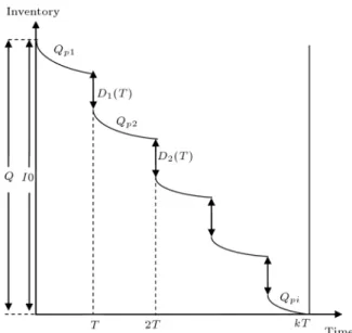
Figure 1. Inventory curve of vendor for deteriorating products.

is price-sensitive while in the second one, deterioration rate is constant and demand rate is time- and price-dependent. The main aim is to extend two models to optimize the dispatch cycle length, selling price, and replenishment quantity for the explained two scenarios such that the total cost is minimized or total prot is maximized. The proposed models in this paper are applicable for every deteriorating product, such as dairy products, vegetables, and whatever is being perished as time passes.

Figure 1 indicates vendor's inventory level in which Q is the replenishment quantity, Qpi is the

deteriorated quantity in each dispatch cycle (i = 1:::k), and Di(T ) shows the demand rate in each dispatch

cycle. The following notations are used: Variables:

T Dispatch cycle length P Wholesale price Q Order quantity Parameters:

Ii(t) The level of inventory in the ith

dispatch cycle at time t

The decaying rate

(t) Time-dependent decaying rate D(p) The price-sensitive demand rate Di(T ) The demand during the ith dispatch

cycle

FD The xed dispatch cost

FR The xed order cost

CD Dispatch cost per unit

CR Purchasing cost per unit

w The waiting cost of product (unit/ time)

h The carrying cost of product (unit/ time)

k The number of dispatching periods during a replenishment cycle v Time-dependent deterioration rate Sj The jth demand arrival time in a

dispatch cycle

Z(t) Deteriorated quantity in the rst model

Qp Deteriorated quantity in the second

model 3. The rst scenario

In this scenario, we assume that decaying rate depends on time and is a continuous function of time, (t) = bt, b 2 [0; 1], and demand rate is price-sensitive and a linear function of wholesale price, D(p) = (a Bp)T . Decision variables that should be determined are dispatch cycle length, wholesale price, and order quantity.

3.1. Mathematical model

Here, a mathematical model of a joint pricing-inventory problem for a time-dependent decaying product using a time-based group dispatching policy is developed. From Figure 1, the changes of inventory level are presented as follows:

(_dI

i(t)

dt = (t)Ii(t) (i 1)D(p); t 2 [(i 1)T; iT ]:

I(kT ) = 0 ₍₁₎

By solving this equation, we have: Ii(t)= (i 1)D(p)

t+bt₆3

e bt22 +I(0)e bt22 : (2)

To obtain the optimum values of variables, rst, the cost function should be modeled. Since each replenish-ment period includes k (random variable) distributing cycles with length T , the expected value of cycle length is E(k)T .

Ordering cost:

The order quantity is demand plus deteriorated prod-uct as shown in Eq. (3):

Q = Z(t) +k 1X

i=1

Di(T ); (3)

where the quantity deteriorated during each cycle is: Z(t) = I(t)without deterioration I(t)with deterioration:

Inventory level without deterioration is obtained using Eq. (5):

I(t)without deterioration= lim

b!0I(t)with deterioration

= l t(i 1)D(p) + I(0): (5)

Thus, using Eqs. (2) and (5) and using I(0) = D(P )(t+

bt3

6 ) + I(t)e

bt2

2 , Eq. (4) changes to:

Z(t) = I(t)(ebt22 1) + (i 1)D(p)bt

3

6 : (6)

Since I(kT ) = 0, deteriorated quantity at the end of each replenishment cycle is:

Z(KT ) = (i 1)D(p)bK₆3T3: (7) Therefore, replenishment quantity is:

Q = Z(KT ) + KD(p)T

= (i 1)D(p)bK₆3T3+ KD(p)T: (8) Finally, the expected replenishment quantity according to Eq. (8) is equal to:

E(Q) = (i 1)D(p)bE(K₆3)T3+ E(k)D(p)T: (9) Thus, the expected related cost is:

E(Rc) = FR+ CRE(Q)

= FR+ CR(a Bp)bE(K 3_)T3

6

+ CRE(k)(a Bp)T: (10)

Dispatch cost:

Based on existing k dispatch cycles and dispatch quantity, which is E(Di(T )), the dispatch cost can be

determined as follows:

dispatch cost = FDE(k) + CDE(k)E(Di(T ))

= FDE(k) + CDE(k)(a bp)T: (11)

Holding cost:

The level of inventory at time t, after substitution of Eq. (8) in Eq. (2), is:

I(t) = D(p)

(kT t) +₆b(k3_T3 _t3_)e bt2 2 :

Utilizing the Taylor series expansion, e bt2

2 = 1 bt2

2 + b2_t4

4 , the cyclic inventory carrying cost is given by:

hE Xk

i=1

( Z _iT

(i 1)TI(t)dt)

!

= hE _Xk

i=1

Z _iT

(i 1)TD(p)

(kT t) +b

6(k3T3 t3)

e bt22

= hE

k2_D(p)T2

2 +

D(p)bk4_T4

12

=hT2₂E(k2)+hbT₁₂4E(k4): (12)

The cost of waiting:

Using the denition of Sj, the waiting time of customer

is T Sj (see Figure 2). Therefore, the cost of waiting

for customer is:

wE(T S1) + (T S2) + ::: + (T SN(T ))

= wE 2 4Di(T )T

D_Xi(T )

n=1

Sn

3

5 = wE(k)T₂2; (13) Using Eqs. (10) to (13), the total cost function is:

Total cost function = FR+ CRT E(k)

+CRbT₆3E(k3)+FDE(k) + CDE(k)T

+hT2₂E(k2)+hbT₁₂4E(k4)+ wE(k)T₂2: (14)

Dividing Eq. (16) over E(k)T yields: T C(p; T; Q) = FR

E(k)T + CR +

CRbT2E(k3)

6E(k) +F_TD + CD +hT E(k

2₎

2E(k)

+hbT_12E(k)3E(k4)+wT₂ : (15)

3.2. Solution method

The following Lemma is presented to derive a solution method.

Lemma 1. The following equations can be used to derive the optimal solutions:

E(k) = Q

T; (16)

E(k2_{) =} Q( Q + 1)

2_T2 ; (17)

E(k3_{) =} Q( Q + 1)( Q + 2)

3_T3 ; (18)

E(k4_{) =} Q( Q + 1)( Q + 2)( Q + 3)

4_T4 : (19)

Proof. Let f(0) denote the distribution function of Di(T ), and f(k)(0) denote the k-fold convolution of

f(0). From k = infnk :Pk_i=1Di(T ) Q

o

, we have P [k k + 1] = f(k)_{(Q) and, thus, P [k k + 1] =}

1 f(k)_{(Q). Since f(0) is a Poisson distribution with}

parameter T , k-fold convolution of f(0) is a Poisson distribution with parameter kT , where:

f(k)_{(Q) =}XQ i=0

(kT )ie kT

i! :

Then, for k = 1; 2; :::, we have: p [K k] = 1

Q

X

i=0

(kT )ie kT

i! ;

of which the right side is a Q-stage P.D.F. with parameter T and expected value of (Q+1)_T .

For simplicity, by using Lemma 1 and substituting

Q = Q+1 and = a bp, the expected long-run average cost changes to:

T C(P; T; Q) = FR(a Bp)_Q + CR(a Bp)

+bCR( Q + 1)( Q + 2)

6(a Bp) +

FD

T +CD(a Bp) +h( Q + 1)₂

+hb( Q + 1)( Q + 2)( Q + 3) 12(a Bp)2

+w(a bp)T₂ ): (20)

Lemma 2. For each couple of T and p, the optimum quantity of Q should satisfy Inequality (21):

Q_{( Q 1) +} b Q( Q+ 1)( Q 1)

(a Bp)

2CR

3h +

( Q_{+ 2)}

2(a Bp)

2FR(a Bp)_h

Q_{( Q+ 1) +}b Q( Q+ 1)( Q+ 2)

(a Bp)

2CR

3h +

( Q_{+ 3)}

2(a Bp)

: (21)

Proof. For each couple of p and T , the optimum quantity of Q should satisfy T C( Q _{1) T C( Q) and}

T C( Q_{+ 1) T C( Q). Using Eq. (20), the optimality}

condition for Q is:

Q_{( Q 1)+}b Q( Q+1)( Q 1)

(a Bp)

2CR

3h +

( Q₊₂₎

2(a Bp)

2FR(a Bp)_h Q_{( Q+ 1)}

+b Q( Q_{(a Bp)}+ 1)( Q+ 2)

2CR

3h +

( Q_{+ 3)}

2(a Bp)

: Lemma 3. The following condition should be satis-ed by the upper bound of Q:

Q_{( Q 1) +} b Q( Q+ 1)( Q 1)

a

2CR

3h +

( Q_{+ 2)}

2a

2F_hRa Q_{( Q+ 1)}

+b Q( Q+ 1)( _a Q+ 2) _2C

R

3h +

( Q_{+ 3)}

2a

: (22) Proof. 2FR(a bp)

h in Eq. (21) is decreasing with

re-spect to p. Therefore, the maximum Q is derived at p = 0.

Theorem 1. The cost function becomes convex is w 2FD

BpT2 +Bbp( Q+1)( _T 3Q+2)

CR

3 +h( Q+3)2

.

Proof. The total cost function is convex if X:H:XT

=P T H P TT 0, where:

H = 2 6 4

@2_{T P}

@p2 @ 2_{T P}

@p@T @2_{T P}

@T @p @

2_{T P}

@T2

3 7 5

= 2 6 4

B2_{b( Q+1)( Q+2)}

3

CR

3 +h( Q+3)2

Bw 2 Bw

2 2FTD3

3 7

5 : (23) Therefore, we have:

XH XT ₌ B2p2b( Q + 1)( Q + 2)

3

CR

3 +

h( Q + 3) 2

+2F_TD BpT w; (24)

and we should show that:

XH XT ₌ B2p2b( Q + 1)( Q + 2)

3

CR

3 +

h( Q + 3) 2

+2F_TD BpT w 0: (25)

Thus, the cost function is convex if and only if: w _BpT2FD₂+Bbp( Q+1)( _{T 3} Q+2)

CR

3 +

h( Q+3) 2

: (26) Using the rst derivative of T C(p; T; Q) with respect to p yields:

@T C(p; T; Q)

@P = B

FR

Q +

wT

2 + CR+ CD bCR( Q + 1)( Q + 2)

62

hb( Q + 1)( Q + 2)( Q + 3) 63

: (27) Moreover, the rst derivative of T C(p; T; Q) with respect to T yields:

@T C(p; T; Q)

@T =

w 2

FD

T2: (28)

Setting Eq. (28) equal to zero gives: p₌ a

B

2FD

BwT2: (29)

After some algebraic calculations, the following equa-tion is derived:

AT4_{+ ET}3_{+ CT + D = 0; (30)}

where:

A = bCR(Q + 1)(Q + 2)w_24F2 2

D ; (31)

E = hbR(Q + 1)(Q + 2)(Q + 3)w_48F3 3

D ; (32)

C =w₂; (33)

D =F_QR + CD+ CR: (34)

Now, we can use the following algorithm to solve the problem.

Step 1. Compute Qmax suing Eq. (22);

Step 2. For ( Q = 1::: Qmax), determine the

coe-cients of the polynomial shown in Eq. (30);

Step 3. Determine all acceptable roots for T using Eq. (30) and MATLAB software;

Step 4. Calculate p for all acceptable roots of T from the previous step;

Step 5. Now, total cost should be calculated using Eq. (20) and convexity should be examined using Theorem 1;

Step 6. In the comparison of the derived total costs, the lowest cost shows the related optimal solutions. 4. The second scenario

In this scenario, we assume that decaying rate is constant and demand rate is time- and price-sensitive and a function of time and selling price D(p; t) = (a bp)T evt _{= T e}vt_{. Decision variables, namely,}

dispatch cycle length, order quantity, and selling price should be determined to optimize the total prot. 4.1. Mathematical modeling

In this scenario, Eqs. (1) and (2) will change to Eqs. (35) and (36) as follows:

dIi(t)

dt = Ii(t) (i 1)D(p; t) t 2 [(i 1)T; iT ];₍₃₅₎

Ii(t) =(i 1)(a bp)e vt

(v + ) h

e(v+)(kT t) ₁i_{: (36)}

Therefore, the order quantity is: Q = I(0) = (a bp)

(v + ) h

According to the description provided for the previous case, E(Di(T )) = evtT = (a bp)evtT and the

expected income is: P E

k 1

X

i=1

Z iT

(i 1)TDi(T )dt

!!

= P E k 1X

i=1

Z iT

(i 1)T(a bp)e vt_{T dt}

!!

= P (a bp)T2_{E(k) +}P (a bp)T3vE(k2)

2 :₍₃₈₎

To derive the cost function, we act as follows. Ordering cost:

The ordering cost of this case, using the logic of the previous case, is:

Q = Qp+ k 1_X

i=1

Di(T ): (39)

Moreover, quantity deteriorated during each cycle is: Qp = I(0) I(KT )

k 1

X

i=1

Di(t); (40)

where:

Q = I(0) = (a bp)_{(v + )} he(v+)kT ₁i_;

I(KT ) = 0; Xk

i=1

Z _iT

(i 1)T(a bp)e vt_{T dt}

! ; and the expected deteriorated quantity is:

E(Qp) = E(I(0)) E(I(KT ))

E Xk

i=1

Z iT

(i 1)T(a bp)e vt_{T dt}

!!

=E(k)T +(v + )T₂ 2E(k2)

+ E(k)T2₊vT3E(k2)

2 : (41)

Finally, using the Taylor series expansion, eT k _{= 1 +}

T k +(T k)₂ 2, Eq. (41) changes to: E(Q) =E(I(0)) = (a bp)E(k)T

+(a bp)(v + )T₂ 2E(k2): (42)

And the expected ordering cost is:

E(Rc) =FR+ CRE(Q) = FR+ CR(a bp)T E(k)

+CR(a bp)T₂2(v + )E(k2): (43) Dispatch cost:

For the distribution cost, similar to the previous case, we have:

E(DC) = FDE(k) + CDE(k)E(Di(T )) = FDE(k)

+ CDE k

X

i=1

Z iT

(i 1)T(a bp)e vt_{T dt}

!!

=FDE(k) + CD(a bp)T2E(k)

+CD(a bp)T₂ 3vE(k2): (44) Carrying cost:

From Eq. (36), the level of inventory at time t is I(t) =

(i 1)(a bp)evt

(v+)

e(v+)(kT t) _{1. Utilizing the Taylor}

series expansion, eT k _{= 1 + T k +}(T k)2

2 , the cyclic

inventory carrying cost is: hE k X i=1 ( Z _iT

(i 1)TI(t)dt)

! =hE _Xk i=1 Z _iT (i 1)T D(p)evt

(v+) (e(v+)(kT t) 1)

dt

= h(a bp)v_{2(v + )}2T2E(k2)

+h(a bp)(v + )T₂ 2E(k2)

h(a bp)vT2_E(k2₎

2(v + ) : (45)

Using Eqs. (38), (43), (44), and (45), the total prot function is:

Total Prot Function= E(k)T2_{p +} pvT3E(k2)

2 8 > > > > > > > > > > < > > > > > > > > > > :

FR+CRT E(k)+CRT

2_(v+)E(k2₎

2

+FDE(k)+CDE(k)T2+CDE(k

2_)vT3

2 hv2_T2_E(k2₎

2(v+) +h(v+)T

2_E(k2₎

2 hvT2_E(k2₎

2(v+) 9 > > > > > > > > > > = > > > > > > > > > > ; : (46)

Dividing the above total prot function by E(k)T , we have:

Total Prot Function = T p +pvT_2E(k)2E(k2) 8 > > > > > > < > > > > > > : FR

E(k)T+CR+CRT (v+)E(k

2₎

2E(k) +FTD

+CDE(k2)vT2

2E(k) hv

2_{T E(k}2₎

2(v+)E(k)+CDT

+h(v+)T E(k_2E(k) 2) hvT E(k_2(v+)E(k)2)

9 > > > > > > = > > > > > > ; : (47)

By substituting E(k) = _{(a bp)e}Q+1vt_T and = a bp, and

assuming Q = Q + 1, the expected long-run average prot changes to:

Total Prot Function = T p +pvT ( _2eQ + 1)_vt 8 > > > > > > < > > > > > > :

FRevt

Q + CR +CR(v+)( 2evtQ+1)+F_TD

+CDT +CDvT ( 2evtQ+1) hv 2_{( Q+1)}

2(v+)evt

+h(v+)( _2evtQ+1) _2(v+)ehv( Q+1)vt

9 > > > > > > = > > > > > > ; : (48)

4.2. Solution method

Lemma 4. For each couple of p and T , the optimum quantity of Q should satisfy Inequality (49):

8 > < > :

(v+) Q_{( Q 1)}

evt +(v+)CR

Q_{( Q+1)}

evt_h v

2_{Q( Q 1)}

(v+)evt

pvT Q_{( Q 1)}

evt_h v Q _{( Q 1)}

(v+)evt +CDvT Q _{( Q 1)}

evt_h

9 > = > ; 2FR(a bp)evt

h 8 > < > :

(v+) Q_{( Q+1)}

evt +(v+)CR

Q_{( Q+1)}

evt_h v

2_{Q( Q+1)}

(v+)evt

pvT Q_{( Q+1)}

evt_h v Q _{( Q+1)}

(v+)evt +CDvT Q _{( Q+1)}

evt_h

9 > = > ;₍₄₉₎: Proof. For each couple of p and T , the optimum quantity of Q should satisfy T P ( Q _{1) T P ( Q) and}

T P ( Q_{+ 1) T P ( Q). Using Eq. (48), the optimality}

condition for Q is obtained as Eq. (49).

Lemma 5. The upper bound of Q satises the following condition:

Q

u( Qu 1) + CR

Q

u( Qu 1)

h

2FRa

h Q

u( Qu+ 1) +CR

Q

u( Qu+ 1)

h : (50)

Proof. The maximum amount of 2FR(a bp)evt

h or the

maximum amount of replenishment is obtained when the demand is maximum. Thus, the maximum quantity of Q is derived at p = v = 0.

Theorem 2. The prot function is concave if and only if FD

h

a + bCD 3bp + v( _2eQ+1)vt

i pT2_:

Proof. The total prot function is concave if X:H:XT _{=P T H P T}T _{0, where:}

H = "

@2_{T P}

@p2 @ 2_{T P}

@p@T @2_{T P}

@T @p @

2_{T P}

@T2

#

= "

2bT a 2bp+bCD+v( _2eQ+1)vt

a 2bp+bCD+v( _2eQ+1)vt 2F_T3D;

# (51) therefore, we have:

X H XT_{= 3bp+a+bC}

D+v( _2eQ+1)_{vt pT}FD₂: (52)

And we should show that: X H XT _{= 3bp + a + bC}

D+v( Q + 1)_2evt

FD

pT2 0: (53)

In order to be sure that the prot function is concave, the following inequality should be held:

FD

a + bCD 3bp +v( Q + 1)_2evt

pT2_{: (54)}

Now, the rst derivative of total prot function with respect to p is:

@T P (p; T; Q)

@P =aT 2bpT +

bFRevt

Q + bCR

+ bT CD+vT ( _2eQ + 1)_vt : (55)

Moreover, the rst derivative with respect to T be-comes:

@T P (p; T; Q)

@T =

FD

T2 CD + p

CDv( Q + 1)

2evt

+pv( Q + 1)

2evt : (56)

By setting Eq. (55) equal to zero, we have: p ₌ a

2b+ FRevt

2T Q + CR

2T + CD

2 +

v( Q + 1)

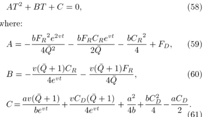
Substitution of Eq. (57) in Eq. (56) yields the following equation:

AT2_{+ BT + C = 0; (58)}

where:

A = bFR_{4 Q}2e₂2vt bFR₂ C_QRevt bC₄R2 + FD; (59)

B = v( Q + 1)C_4evt R v( Q + 1)F_{4 Q} R; (60)

C =av( _beQ + 1)_vt +vCD_4e( Q + 1)_vt +a_4b2+bCD2

4

aCD

2 ₍₆₁₎: Eq. (58) is a quadratic polynomial of which the dis-criminant is:

= B2 _{4AC: (62)}

Based on the sign of , the following cases can occur:

1. When > 0, two real roots exist;

2. When = 0, a single root exists;

3. When < 0, there is no real root.

Now, we can use the following solution procedure to solve the problem:

Step 1. Determine Qmax using Eq. (50);

Step 2. For ( Q = 1::: Qmax), determine the

coe-cients of polynomial (58);

Step 3. Determine all acceptable roots of period length using Eq. (58) and MATLAB;

Step 4. Determine p for all acceptable roots of period length from the previous step;

Step 5. For all combinations of order quantity, selling price, and period length, calculate the related total prot and check the concavity using Theorem 2; Step 6. By comparison of the obtained total prots, the related optimal decision variables can be applied. 5. Practical and computational results

Consider a milk producer company for which deteri-orating rate is linearly time-proportional, (t) = bt, b 2 [0; 1], and demand rate is price-sensitive and is a linear function of wholesale price, D(p) = (a Bp)T . Moreover, deterioration rate may be constant and demand rate can be time- and price-sensitive and a function of time and selling price D(p; t) = (a bp)T evt _{= T e}vt_{. These two conditions can}

be analyzed using the rst and the second models developed in this paper. Decision variables, namely, cycle length, selling price, and order quantity, should be determined such that total cost is minimized using the proposed solution method.

5.1. Example 1

For the rst developed model, consider FD= 5, FR=

40, a = 20, CD= 3, h = 1, w = 50, B = 0:02, = 0:04,

b = 0:05, and CR= 40.

Step 1. Using Eq. (22), Q = 25;

Step 2. From Q = 1 to 25, the values of Eqs. (31) to (34) are determined;

Step 3. All acceptable real roots of cycle length are determined and reported in Table 1;

Step 4. For all acceptable values of T , the wholesale prices are determined (see Table 1);

Step 5. For all groups of decision variables, the concavity of the objective function is checked and the related values are shown in Table 1;

Step 6. The lowest cost, i.e. T C _{= 149:2175,}

corresponds to Q _{= 10, T = 0:3179, and P =}

90:1049.

5.2. Example 2

Now, consider FD = 5, CD = 3, h = 1, b = 0:04,

FR = CR = 40, w = 50, v = 0:98, = 0:04, and

a = 20.

Step 1. From Eq. (50), Q = 40;

Step 2. From Q = 1 to 40, the values of Eqs. (59) to (61) are calculated;

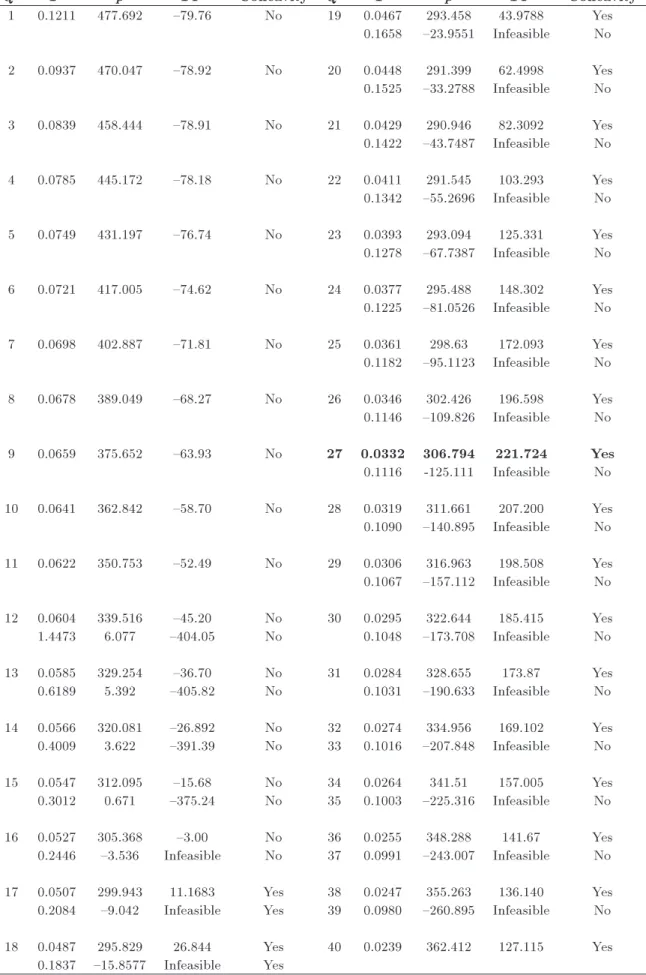
Step 3. All acceptable roots of cycle length are calculated and reported in Table 2;

Table 1. Results for the rst example.

Q T p T C Convexity

1 1.1846 99.2874 36.4358 No 2 0.8894 98.7358 44.4573 No 3 0.7235 98.0896 54.0442 No 4 0.6124 97.3336 64.5559 No 5 0.5312 96.4561 76.0043 No 6 0.4690 95.4537 88.4376 No 7 0.4196 94.3203 101.9309 No 8 0.3794 93.0529 116.5323 No 9 0.3460 91.6469 132.2982 No 10 0.3179 90.1049 149.2175 Yes 11 0.2939 88.4229 167.3233 Yes 12 0.2732 86.6020 186.6376 Yes 13 0.2552 84.6454 207.1067 Yes 14 0.2393 82.5372 228.8869 Yes 15 0.2253 80.2995 251.7767 Yes 16 0.2127 77.8963 276.1084 Yes 17 0.2015 75.3708 301.4834 Yes 18 0.1914 72.7029 328.0874 Yes 19 0.1822 69.8767 356.0674 Yes 20 0.1739 66.9325 385.0502 Yes 21 0.1662 63.7976 415.7086 Yes 22 0.1592 60.5439 447.3766 Yes 23 0.1528 57.1695 480.0718 Yes 24 0.1469 53.6600 513.9276 Yes 25 0.1414 49.9849 549.2252 Yes

Table 2. Results for the second example.

Q T p T P Concavity Q T p T P Concavity

1 0.1211 477.692 {79.76 No 19 0.0467 293.458 43.9788 Yes 0.1658 {23.9551 Infeasible No 2 0.0937 470.047 {78.92 No 20 0.0448 291.399 62.4998 Yes 0.1525 {33.2788 Infeasible No 3 0.0839 458.444 {78.91 No 21 0.0429 290.946 82.3092 Yes 0.1422 {43.7487 Infeasible No 4 0.0785 445.172 {78.18 No 22 0.0411 291.545 103.293 Yes 0.1342 {55.2696 Infeasible No 5 0.0749 431.197 {76.74 No 23 0.0393 293.094 125.331 Yes 0.1278 {67.7387 Infeasible No 6 0.0721 417.005 {74.62 No 24 0.0377 295.488 148.302 Yes 0.1225 {81.0526 Infeasible No

7 0.0698 402.887 {71.81 No 25 0.0361 298.63 172.093 Yes

0.1182 {95.1123 Infeasible No 8 0.0678 389.049 {68.27 No 26 0.0346 302.426 196.598 Yes 0.1146 {109.826 Infeasible No 9 0.0659 375.652 {63.93 No 27 0.0332 306.794 221.724 Yes

0.1116 -125.111 Infeasible No 10 0.0641 362.842 {58.70 No 28 0.0319 311.661 207.200 Yes 0.1090 {140.895 Infeasible No 11 0.0622 350.753 {52.49 No 29 0.0306 316.963 198.508 Yes 0.1067 {157.112 Infeasible No 12 0.0604 339.516 {45.20 No 30 0.0295 322.644 185.415 Yes 1.4473 6.077 {404.05 No 0.1048 {173.708 Infeasible No 13 0.0585 329.254 {36.70 No 31 0.0284 328.655 173.87 Yes 0.6189 5.392 {405.82 No 0.1031 {190.633 Infeasible No 14 0.0566 320.081 {26.892 No 32 0.0274 334.956 169.102 Yes 0.4009 3.622 {391.39 No 33 0.1016 {207.848 Infeasible No 15 0.0547 312.095 {15.68 No 34 0.0264 341.51 157.005 Yes 0.3012 0.671 {375.24 No 35 0.1003 {225.316 Infeasible No

16 0.0527 305.368 {3.00 No 36 0.0255 348.288 141.67 Yes

0.2446 {3.536 Infeasible No 37 0.0991 {243.007 Infeasible No 17 0.0507 299.943 11.1683 Yes 38 0.0247 355.263 136.140 Yes 0.2084 {9.042 Infeasible Yes 39 0.0980 {260.895 Infeasible No 18 0.0487 295.829 26.844 Yes 40 0.0239 362.412 127.115 Yes

Step 4. p is determined for all acceptable roots of T (see Table 2);

Step 5. For all groups of decision variables, the concavity of the objective function is checked and the related values are shown in Table 2;

Step 6. The highest prot, i.e. T P _{= 221:724,}

corresponds to Q _{= 27, T = 0:0332, and P =}

306:794.

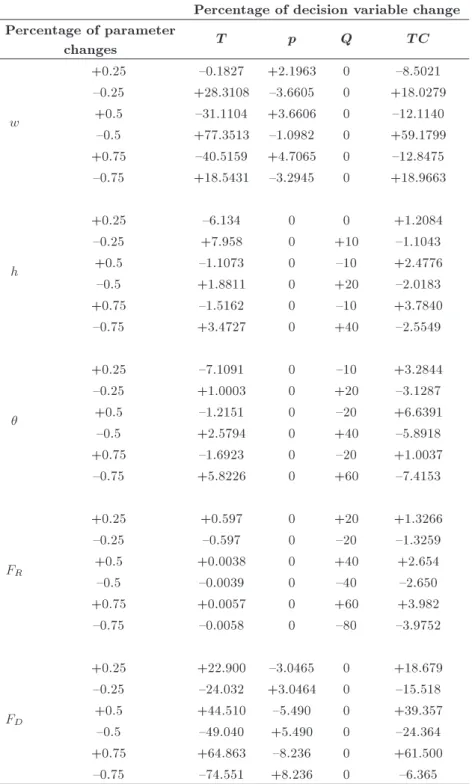
6. Sensitivity analysis

To examine the sensitivity of the variables with respect to input of the model, sensitivity analysis is performed and results are shown in Tables 3 and 4. In both tables, zero represents that changes of the parameters have no eect on optimal solution.

In the rst model, sensitivity analysis has been conducted on the parameters w, FD, FR, h, and ,

Table 3. Eects of parameter changes on optimal values of the rst model. Percentage of decision variable change Percentage of parameter

changes T p Q T C

w

+0.25 {0.1827 +2.1963 0 {8.5021

{0.25 +28.3108 {3.6605 0 +18.0279

+0.5 {31.1104 +3.6606 0 {12.1140

{0.5 +77.3513 {1.0982 0 +59.1799

+0.75 {40.5159 +4.7065 0 {12.8475 {0.75 +18.5431 {3.2945 0 +18.9663

h

+0.25 {6.134 0 0 +1.2084

{0.25 +7.958 0 +10 {1.1043

+0.5 {1.1073 0 {10 +2.4776

{0.5 +1.8811 0 +20 {2.0183

+0.75 {1.5162 0 {10 +3.7840

{0.75 +3.4727 0 +40 {2.5549

+0.25 {7.1091 0 {10 +3.2844

{0.25 +1.0003 0 +20 {3.1287

+0.5 {1.2151 0 {20 +6.6391

{0.5 +2.5794 0 +40 {5.8918

+0.75 {1.6923 0 {20 +1.0037

{0.75 +5.8226 0 +60 {7.4153

FR

+0.25 +0.597 0 +20 +1.3266

{0.25 {0.597 0 {20 {1.3259

+0.5 +0.0038 0 +40 +2.654

{0.5 {0.0039 0 {40 {2.650

+0.75 +0.0057 0 +60 +3.982

{0.75 {0.0058 0 {80 {3.9752

FD

+0.25 +22.900 {3.0465 0 +18.679

{0.25 {24.032 +3.0464 0 {15.518

+0.5 +44.510 {5.490 0 +39.357

{0.5 {49.040 +5.490 0 {24.364

+0.75 +64.863 {8.236 0 +61.500

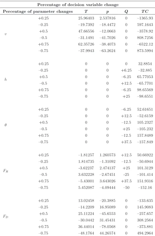
Table 4. Eects of parameter changes on optimal values of the rst model. Percentage of decision variable change

Percentage of parameter changes T p Q T C

v

+0.25 25.96403 2.537816 0 {1365.93

{0.25 {19.7392 {18.4472 0 597.1643

+0.5 47.66556 {12.0663 0 {3578.92

{0.5 {31.1491 {41.7026 0 808.7256

+0.75 62.35726 {38.4073 0 {6522.12

{0.75 {37.9943 {63.2624 0 873.5994

h

+0.25 0 0 0 32.8854

{0.25 0 0 +6.25 {32.885

+0.5 0 0 {6.25 65.77053

{0.5 0 0 +12.5 {65.7701

+0.75 0 0 {6.25 98.65569

{0.75 0 0 +25 {98.6551

+0.25 0 0 {6.25 52.61651

{0.25 0 0 +12.5 {52.6159

+0.5 0 0 {12.5 105.2327

{0.5 0 0 +25 {105.232

+0.75 0 0 {12.5 157.8489

{0.75 0 0 +37.5 {157.849

FR

+0.25 {1.81257 1.260573 +12.5 50.66922 {0.25 1.814735 {1.31092 {12.5 {50.6944 +0.5 -3.62237 2.474137 +25 101.3129 {0.5 3.632228 {2.67451 -25 {101.414 +0.75 {5.43001 3.643026 +37.5 151.9316 {0.75 5.452087 {4.09444 {50 {152.16

FD

+0.25 13.02458 {20.3885 0 {133.635

{0.25 {14.2209 16.95089 0 145.9083

+0.5 25.11224 {45.6553 0 {257.657

{0.5 {30.0442 31.45431 0 308.2564

+0.75 36.44014 {78.0568 0 {373.881

{0.75 {48.1764 44.26574 0 494.2964

since they have more important eects on the prot, decision making, and managerial insights. According to Tables 3 and 4, when holding cost increases, order quantity and dispatch cycle length decrease, and total cost increases. However, when w increases, selling price increases, and period length and total cost decrease. Moreover, when FR becomes larger, order quantity,

total cost, and dispatch cycle length increase.

When FDbecomes larger, total cost and dispatch

cycle length increase and selling price decreases and

when decaying rate increases, total cost increases and both order quantity and dispatch cycle length decrease. It is noticeable that QBC causes a considerable de-crease in cost. Table 3 represents the sensitivity analy-sis for the rst model. For the second model, sensitivity analysis has been conducted on the parameters v , FD,

FR, h, and . Table 4 represents the sensitivity analysis

for the second model. According to the results, when the waiting cost is high, the vendor dispatches smaller orders in order to decrease the waiting costs, because

the waiting time of customers increases as dispatch cycle length becomes larger.

7. Conclusion

In this paper, two mathematical models were presented for an integrated pricing-inventory problem of a single decaying product (since the number of deteriorating products increased every day) and optimum quantities of period length, order quantity, and selling price were obtained under two dierent scenarios. Then, by using several lemmas and theorems, the convexity and concavity of the functions of the two extended models were proved and dierent solution methods (algorithms) were developed to solve the models. In order to decrease the cost of transportation, time-based consolidation policy was applied. The devel-oped models in this paper were comprehensive and considered as dierent forms of demand functions and deteriorating rates. Also, all costs of an inventory system were taken into consideration in the extended models. Finally, two examples were provided to show the applicability of the proposed policies. This model was developed under certain environment, and shortage was not permitted. Also, a single-stage problem was considered and developed and no contract was used between the stockholders. Therefore, for the future studies, permissible delay in payments contract and considering promotions, stochastic or fuzzy demand, multi-level supply chain, and permitted shortage could be of interest.

Acknowledgment

The rst author would like to thank the nancial support of University of Tehran for this research under grant number 30015-1-04.

References

1. Cetinkaya, S. and Lee, C.Y. \Stock replenishment and shipment scheduling for vendor-managed inventory systems", Management Science, 46(2), pp. 217-232 (2000).

2. Whitin, T. \Inventory control and price theory", Management Science, 2, pp. 61-68 (1955).

3. Chen, F.Y., Wang, T., and Xu, T.Z. \Integrated inventory replenishment and temporal shipment con-solidation: A comparison of quantity-based and time-based models", Annals of Operations Research, 135, pp. 197-210 (2005).

4. Ray, S., Song, Y., and Verma, M. \Comparison of two periodic review models for stochastic and price-sensitive demand environment", International Journal of Production Economics, 128, pp. 209-222 (2010).

5. Huang, Y., Huang, G.Q., and Newman, S.T. \Coordi-nating pricing and inventory decisions in a multi-level supply chain: A game theoretic approach", Trans-portation Research Part E, 47, pp. 115-129 (2011).

6. Polatoglu, L.H. \Optimal order quantity and pricing decisions in single-period inventory systems", Interna-tional Journal of Production Economics, 23, pp. 175-185 (1991).

7. Zhu, S.X. \Joint pricing and inventory replenish-ment decisions with returns and expediting", Euro-pean Journal of Operation Research, 216, pp. 105-112 (2012).

8. You, P.S., Ikuta, S., and Hsieh, Y.C. \Optimal order-ing and pricorder-ing policy for an inventory system with trial periods", Applied Mathematical Modeling, 34, pp. 3179-3188 (2012).

9. Su, Y. and Geunes, J. \Price promotions, operations cost, and prot in a two-stage supply chain", Omega, 40, pp. 891-905 (2012).

10. Mutlu, F. and Cetinkaya, S. \Pricing decisions in a carrier-retailer channel under price-sensitive demand and contract-carriage with common-carriage option", Transportation Research Part E, 51, pp. 28-40 (2013).

11. Maddah, B. and Bish, E.K. \Joint pricing, assortment, and inventory decisions for a retailer's product-line", Naval Research Logistics, 54, pp. 315-330 (2007).

12. Maity, K. and Maiti, M. \A numerical approach to a multi-objective optimal inventory control problem for deteriorating multi-items under fuzzy ination and discounting", Computer and Mathematics with Applications, 55, pp. 1794-1807 (2008).

13. Yu, Y., Wang, Z., and Liang, L. \A vendor managed inventory supply chain with deteriorating raw materi-als and products", International Journal of Production Economics, 136, pp. 266-274 (2012).

14. Hongjie, L., Ruxian, L., Zhigao, L., and Ruijiang, W. \Study on the inventory control of deteriorating items under VMI model based on bi-level programming", Expert Systems with Application, 38, pp. 9287-9295 (2011).

15. Mahata, G.C. \An EPQ-based inventory model for exponentially deteriorating items under retailer partial trade credit policy in supply chain", Expert Systems with Application, 39, pp. 3537-3550 (2012).

16. Taleizadeh, A.A. and Nematollahi, M. \An inventory control problem for deteriorating items with backo-rdering and nancial considerations", Applied Math-ematical Modeling, 38(1), pp. 93-109 (2013a).

17. Lee, C.F. and Chung, C.P. \An inventory model for deteriorating items in a supply chain with system dynamics analysis", Procedia-Social and Behavioral Sciences, 40, pp. 41-51 (2012).

18. Cetinkaya, S. and Bookbinder, J.H. \Stochastic models for the dispatch of consolidated shipments", Trans-portation Research-Part B, 37, pp. 747-768 (2003).

19. Cetinkaya, S., Mutlu, F., and Lee, C.Y. \A comparison of outbound dispatch policies for integrated inventory and transportation decisions", European Journal of Operation Research, 171, pp. 1094-1112 (2006).

20. Wong, W.H., Lawrence, C.L., and Hui, Y.V. \Air-freight forwarder shipment planning: A mixed 0-1 model and managerial issues in the integration and consolidation of shipments", European Journal of Operation Research, 193, pp. 86-97 (2009).

21. Marklund, J. \Inventory control in divergent supply chains with time-based dispatching and shipment con-solidation", Naval Research Logistics, 58, pp. 59-71 (2010).

22. Howard, C. and Marklund, J. \Evaluation of stock allocation policies in a divergent inventory system with shipment consolidation", European Journal of Operation Research, 211, pp. 298-309 (2011).

23. Taleizadeh, A.A., Moghadasi, H., Niaki, S.T.A., and Eftekhari, A.K. \An EOQ-joint replenishment policy to supply expensive imported raw materials with pay-ment in advance", Journal of Applied Science, 8(23), pp. 4263-4273 (2009).

24. Taleizadeh, A.A., Niaki, S.T.A., and Naja, A.A. \Multi product single machine production system with stochastic scraped production rate, partial back order-ing and service level constraint", Journal of Compu-tational and Applied Mathematics, 233(8), pp. 1834-1849 (2010a).

25. Taleizadeh, A.A., Naja, A.A., and Niaki, S.T.A. \Multi product EPQ model with scraped items and limited production capacity", Scientia Iranica, Trans-action E, 17(1), pp. 58-69 (2010b).

26. Ulku, M.A. and Bookbinder, J.H. \Modelling shipment consolidation and pricing decisions for a manufacturer-distributor", International Journal of Revenue Man-agement, 6(1) (2012).

27. Sajadieh, M.S. and Jokar, M.R.A. \Optimizing ship-ment, ordering and pricing policies in a two-stage sup-ply chain with price-sensitive demand", Transportation Research - Part E, 45, pp. 564-571 (2009).

28. Olsson, F. \Analysis of inventory policies for perishable items with xed leadtimes and lifetimes", Annals of Operations Research, 217(1), pp. 399-423 (2014).

29. Herbon, A., Levner, E., and Cheng, T.C.E. \Per-ishable inventory management with dynamic pricing using time-temperature indicators linked to automatic detecting devices", International Journal of Produc-tion Economics, 147, pp. 605-613 (2014).

30. Taleizadeh, A.A. \An economic order quantity model with consecutive payments for deteriorating items", Applied Mathematical Modeling, 38, pp. 5357-5366 (2014a).

31. Taleizadeh, A.A. \An economic order quantity model with partial backordering and advance payments for an evaporating item", International Journal of Pro-duction Economic, 155, pp. 185-193 (2014b).

32. Diabat, A., Abdallah, T., and Le, T. \A hybrid tabu search based heuristic for the periodic distribution inventory problem with perishable goods", Annals of Operations Research, 242(2), pp. 1-26 (2014).

33. Lu, L., Zhang, J., and Tang, W. \Optimal dy-namic pricing and replenishment policy for perishable items with inventory-level-dependent demand", Inter-national Journal of Systems Science, 47(6), pp. 1480-1494 (2016).

34. Gallego, G. and Hu, M., Dynamic Pricing of Perish-able Assets under Competition Management Science, 60(5), pp. 1241-1259 (2014) .

35. Tayal, S.H., Singh, S.R., and Sharma, R. \An in-tegrated production inventory model for perishable products with trade credit period and investment in preservation technology", International Journal of Mathematics in Operational Research, 8(2), pp. 137-163 (2016).

36. Taleizadeh, A.A., Satarian, F., and Jamil, A. \Optimal multi-discount selling prices schedule for deteriorat-ing product", Scientia Iranica, 22(6), pp. 2595-2603 (2015).

37. Maleki Vishkaei, B., Pasandideh, S.H.R., and Farhangi, M. \The 100% screening economic order quantity model under shortage and delay in payment", Scientia Iranica, 21(6), pp. 2429-2435 (2015).

38. Taleizadeh, A.A., Niaki, S.T.A., and Aryanezhad, M.B. \Replenish-up-to multi chance-constraint inven-tory control system with stochastic period lengths and total discount under fuzzy purchasing price and hold-ing costs", International Journal of System Sciences, 41(10), pp. 1187-1200 (2010c).

39. Taleizadeh, A.A., Wee, H.M., and Sadjadi, S.J. \Multi-product \Multi-production quantity model with repair failure and partial back-ordering", Computers and Industrial Engineering, 59(1), pp. 45-54 (2010d).

40. Taleizadeh, A.A., Niaki, S.T.A., Aryanezhad, M.B., and Fallah-Tafti, A. \A genetic algorithm to optimize multi-product multi-constraint inventory control sys-tems with stochastic replenishments and discount", In-ternational Journal of Advanced Manufacturing Tech-nology, 51, (1-4), pp. 311-323 (2010e).

41. Taleizadeh, A.A., Barzinpour, F., and Wee, H.M. \Meta-heuristic algorithms to solve the fuzzy single pe-riod problem", Mathematical and Computer Modeling, 54(5-6), pp. 1273-1285 (2011f).

42. Taleizadeh, A.A., Cardenas-Barron, L.E., Biabani, J., and Nikousokhan, R. \Multi products single machine EPQ model with immediate rework process", Inter-national Journal of Industrial Engineering Computa-tions, 3(2), pp. 93-102 (2012a).

43. Taleizadeh, A.A., Pentico, D.W., Aryanezhad, M.B., and Ghoreyshi, M. \An economic order quantity model with partial backordering and a special sale price", European Journal of Operational Research, 221(3), pp. 571-583 (2012b).

44. Taleizadeh, A.A., Niaki, S.T., Aryanezhad, M.B., and Shai, N. \A hybrid method of fuzzy simulation and genetic algorithm to optimize multi-product single-constraint inventory control systems with stochastic replenishments and fuzzy-demand", Information Sci-ence, 220(20), pp. 425-441 (2013b).

45. Taleizadeh, A.A., Pentico, D.W., Jabalameli, M.S., and Aryanezhad, M.B. \An economic order quantity model with multiple partial prepayments and partial backordering", Mathematical and Computer Modeling, 57(3-4), pp. 311-323 (2013c).

46. Taleizadeh, A.A., Mohammadi, B., Cardenas-Barron, L.E., and Samimi, H. \An EOQ model for perishable product with special sale and shortage", International Journal of Production Economics, 145(1), pp. 318-338 (2013d).

47. Taleizadeh, A.A., Jalali-Naini, S.G.H., Wee, H.M., and Kuo, T.C. \An imperfect, multi product production system with rework", Scientia Iranica, 20(3), pp. 811-823 (2013e).

48. Taleizadeh, A.A. and Pentico, D.W. \An economic order quantity model with known price increase and partial backordering", European Journal of Opera-tional Research, 28(3), pp. 516-525 (2013f).

49. Teimoury, R. and Kazemi, S.M.M. \An integrated pricing and inventory model for deteriorating products

in a two stage supply chain under replacement and shortage", Scientia Iranica, 24(1), pp. 342-354 (2017). Biographies

Ata Allah Taleizadeh is an Associate Professor in the School of Industrial Engineering, College of Engineering at University of Tehran in Iran. He received his PhD degree in Industrial Engineering from Iran University of Science and Technology. Moreover, he received his BSc and MSc degrees both in Industrial Engineering from Azad University of Qazvin and Iran University of Science and Technology, respectively. His research interests include inventory control and production planning, pricing and revenue optimization, and Game theory. He has published several papers in reputable journals and book chapters, and is now serving as the editor/editorial board member for a number of international journals.

Arezu Rasouli-Baghban received her MSc degree in Industrial Engineering from South Tehran Branch of Islamic Azad University and BSc degree in Mathemat-ics from K. N. Toosi University of Technology. Her research interests include supply chain management, inventory control, and operation research.