Sharif University of Technology
Scientia IranicaTransactions E: Industrial Engineering http://scientiairanica.sharif.edu
Simulation-based optimization of a stochastic supply
chain considering supplier disruption: Agent-based
modeling and reinforcement learning
A. Aghaie
and M. Hajian Heidary
Department of Industrial Engineering, K.N. Toosi University of Technology, Pardis Street, Mollasadra Street, Vanaq Square, Tehran, 1999143344, Iran.
Received 20 June 2017; received in revised form 6 April 2018; accepted 21 July 2018
KEYWORDS Supply chain management; Simulation-based optimization; Reinforcement Learning (RL); Demand uncertainty; Supplier disruption.
Abstract. Many researchers and practitioners in recent years have become attracted to the idea of investigating the role of uncertainty in the supply chain management concept. In this paper, a multi-period stochastic supply chain with demand uncertainty and supplier disruption is modeled. In the model, two types of retailers including sensitive and risk-neutral retailers with many capacitated suppliers are considered. Autonomous retailers have three choices to satisfy demands: ordering from primary suppliers, reserved suppliers, and spot market. The goal is to nd the best behavior of the risk-sensitive retailer regarding the forward and option contracts during several contract periods based on the prot function. Hence, an agent-based simulation approach has been developed to simulate the supply chain and transactions between retailers and unreliable suppliers. In addition, a Q-learning approach (as a method of reinforcement learning) has been developed to optimize the simulation procedure. Furthermore, dierent congurations of the simulation procedure are analyzed. The R-netlogo package is used to implement the algorithm. In addition, a numerical example has been solved by the proposed simulation-optimization approach. Several sensitivity analyses are conducted regarding dierent parameters of the model. A comparison between the numerical results and a genetic algorithm shows the signicant eciency of the proposed Q-leaning approach.
© 2019 Sharif University of Technology. All rights reserved.
1. Introduction
The importance of uncertainty and the consequent cost of ignoring it has led to a shift from deterministic congurations of the supply chain to the stochastic models. One of the most important problems in the stochastic supply chain ordering management is the newsvendor (NV) problem. The basic form of the *. Corresponding author. Tel.: +98 21 84063363;
Fax: +98 21 88674858
E-mail address: [email protected] (A. Aghaie) doi: 10.24200/sci.2018.20789
NV problem consists of a buyer and a seller in which the buyer must decide on the amount of ordering from the seller when demand of the customers is not predetermined. In the basic form, the buyer only has the overall information about customer demand such as the distribution function. In addition, the decision is made only in one period. The objective is to optimize the prot of the buyer. Two extensions of the problem have been done by the researchers: the Multi-period NV Problem (MNVP) and the NV Problem with Supplier Disruption (NVPSD). In the MNVP, the buyer(s) decides on the amount of ordering from the seller(s) at the beginning of each period. The buyer(s) decides on the amount of orders based
on the uncertain demands of their customers and the remaining inventory from the previous period. In the NVPSD (which often consists of one period), the buyer(s) decides on the amount of orders based on uncertain customer demand and the remaining xed capacities of the sellers. In the related literature of the NVPSD, it is usually assumed that the network consists of many uncertain sellers and one buyer (e.g., [1-3]). On the other hand, in the literature of the MNVP, some researchers have assumed many buyers and one seller in their network [4]. Thus, inspired by Kim et al. [4] and the related literature of the NVPSD, this study denes a many-to-many relation here. In the new conguration, each buyer decides on the amount of the order from an uncertain seller at the beginning of each time unit. In addition, it is more practical to make a decision within a contract period that consists of several time units while demand varies during each time unit, instead of making decisions at the beginning of each time unit. This has not been elaborated in the context of the NV problem.
Practical applications of the NVPSD arise partic-ularly in the decisions regarding global sourcing. The following example claries the importance of the deci-sions of the buyers in the global sourcing with uncertain suppliers. For instance, an automotive component manufacturer had expected to save 4-5 million dollars a year resulting from sourcing of a product from Asia instead of Mexico. Port congestion and chartering air-craft to y the products from Asia caused a 20-million-dollar loss [5]. This example and other practical appli-cations of sourcing decision, especially when a contract is signed between a retailer and a supplier, highlight the importance of studying sourcing decisions in an uncertain supply chain (the MNVP and the NVPSD). Extension of the NVP to the MNVP or NVPSD makes the problem much more challenging. Suppliers with uncertain and limited capacities and inventory positions of the retailers pose a greater challenge to the basic NVP. To the best of our knowledge, the combination of the MNVP and the NVPSD has not been researched before. This combined problem is called MNVPSD. In addition, to avoid shortages, it is assumed that retailers have two options after the real-ization of the demand in each time unit: buying from a reserved supplier and if the amount of reservation is not sucient to satisfy the demand, retailers have another option to buy from the spot market [1]. These options are common in the industries such as semiconductors, telecommunications, and pharmaceuticals. Details of the problem are discussed in Section 3. A two-stage decision-making is required to solve the problem in each time unit, in which an order must be placed before the realization of the demand and subsequent decisions regarding the ordering from the reserved supplier, and the spot market must be made after the realization.
Solving a large-sized NVPSD is computationally not tractable [1-3]. In addition, heuristic approaches are common tools for solving the MNVP [4]. Thus, it could be concluded that solving the MNVPSD by an exact approach or a common optimization software
is more dicult. In this regard and considering
autonomous retailers, an agent-based Q-learning is developed and implemented to solve the problem. In the following, the basics of agent-based modeling and reinforcement learning are introduced.
1.1. Agent-based modeling
Agent-based modeling is a bottom-up approach among dierent simulation modeling approaches in which agents interact with each other and, also, with the environment [6]. Agent-based modeling facilitates sim-ulation optimization loop of the related optimization of behavioral parameters [7]. An agent-based simulation model consists of a certain number of agents and their behaviors, aecting their property, other actions, and their environment.
Based on a research, dierent approaches to developing an ABMS could be divided into four cate-gories [8]: individual ABMS (agents have a prescribed behavior and there is no interaction between agents and the environment), autonomous ABMS (agents have autonomous behavior and there is no interaction be-tween agents and the environment), interactive ABMS (agents have the same behavior as autonomous ABMS, yet the interaction between agents and environment is possible), and adaptive ABMS (behavior of the agents is the same as interactive ABMS, yet agents can change their behavior during the simulation). To make an intelligent network of agents, researchers usually add the learning feature to their models. In this regard, Reinforcement Learning (RL) has been adopted in our modeling.
1.2. Reinforcement Learning (RL)
Reinforcement Learning (RL) is a machine learning approach and is a proper approach to optimizing multi-agent models [9]. Indeed, an RL algorithm is a learning mechanism to map the situations to actions [10]. In the RL, there is a set of states (S), a set of actions (A), and a reward function (R). In the stochastic environments, a stochastic subset of the problem could be handled as a Markov or semi-Markov model [11]. In general, a Markov process is formulated as follows:
Pr(st+1= s; rt+1= rj st; at; :::; s0; a0)
= Pr(st+1= s; rt+1= rj st; at): (1)
The above-mentioned formula shows the memory-less characteristic of the Markov process, which explains that the state and reward at time (t + 1) only depend on the last time unit (t). RL is an algorithm with the
ability to solve decision problems with Markov prop-erty. Basically, the states dened in RL algorithm must have Markov property; in case they do not have Markov property, RL may represent a good approximation of the solution [10].
One of the most popular methods for implement-ing RL and the optimal set of \action states" is Q-learning (as a model-free algorithm). In this regard, a Q-function must be dened. A Q-function in RL algorithm could be dened as the expected value of the discounted reward gained from a specic set of states and actions:
Q(s; a) = E 0 @T t 1X
=0
r
t++1j st= s; at= a
1 A :
(2) Since modeling all the dynamics of the system is not possible in most real-world problems, usually, an estimation of the Q-function is used to model the prob-lem (e.g., by using an iterative Q-learning algorithm). At the end of the learning process, the action with the largest value of Q-function is chosen for all the current states. In Section 4, the learning algorithm is described.
The remaining parts of the paper are organized as follows: In the next section, related works are reviewed. In Section 3, the mathematical formulation of the problem is presented. In Section 4, based on the formulation presented in Section 3, an agent-based RL approach is elaborated. In Section 5, results of applying the proposed framework to an illustrative example are shown. Finally, in the last section, concluding remarks are presented.
2. Literature review
The main focus of this research is to analyze the risk behavior of the retailers in the stochastic supply chain by simulation optimization approaches. To design a stochastic supply chain, the MNVP is extended by multiple uncertain suppliers, and the NVPSD is ex-tended by multiple periods. Additionally, a simulation optimization approach is developed based on a multi-agent system.
The NV problem is a common problem in the inventory management. Many researchers have stud-ied this problem and developed it in dierent ways. According to the assumptions considered in this paper, related researches of NV problem, which considered these two assumptions, are reviewed: multi-period modeling and unreliable suppliers.
In the past years, some of the researchers devel-oped the NVP with one retailer and multiple unreliable
suppliers. There are a few papers regarding the
supplier disruption in the NV conguration [12].
Recently, some of the researchers focused more on the NV model with unreliable suppliers. Among them, Ray and Jenamani [2] proposed a one-period NV opti-mization model with one retailer and many unreliable capacitated suppliers. They solved the problem with a simulation optimization approach using discrete event simulation and genetic algorithm. They asserted that the problem was computationally not tractable by in-creasing the number of suppliers. Afterwards, Ray and Jenamani [3] proposed a heuristic approach to solve the problem that they developed in their previous work. They suggested that an important future extension of their problem is considering \multiple periods in the modeling". Merzifonluoglu and Feng [12] presented an-other important research regarding the development of NV model with unreliable suppliers. They proposed a heuristic approach to solve a one-period uncapacitated NV model. They suggested using risk-sensitive (versus risk neutral) modeling. Afterwards, Merzifonluoglu [1] developed the model of Merzifonluoglu and Feng [12] by adding some assumptions such as option contracts. She also modeled the concept of the capacity reservation in the NV model [13,14].
Based on the above researches, our assumptions regarding multiple unreliable capacitated suppliers were adopted from Ray and Jenamani [2], Merzifon-luoglu [1]; in addition, option contract assumption was adopted from Merzifonluoglu [1]. As suggested by Ray and Jenamani [3], the problem of ordering from unreliable capacitated suppliers has been extended to multiple periods in this paper. In the following, related works are presented.
Developing a multi-period model for the NVP is another extension to the common NVP. In this regard, applying utility function, Bouakiz and So-bel [15] performed a risk analysis of the MNVP. One of the main parts of the literature (relating to the MNVP) is about the estimation of demand distribution with dierent approaches. Another main part of the literature is about modeling uncertainties in the NV problem, e.g., uncertainty of the supplier capacity [16], uncertainty of the selling price [17], and uncertainty of the demand [4]. Additionally, Kim et al. [4] developed a MNVP with a distributor and many retailers. Hence, inspired by the extensions of Ray and Jenamani [2] and Merzifonluoglu [1], their assumptions were mixed and, then, a multi-period NV model was developed with many retailers and many unreliable capacitated suppliers considering option contracts. In addition, it was assumed that retailers had a risk-sensitive behavior.
One of the best tools to solve a complex decision-making problem, such as inventory replenishment prob-lems, is simulation optimization. Jalali and Nieuwen-huyse [18] reviewed and classied previous works on the simulation optimization technique in inventory
management. They classied related works into two categories: domain and methodology focused. Based on their classication, domain-focused works mainly contribute to the modeling of the inventory. Works focused on the methodology attempt to solve a simple problem with a new approach. They did not address agent-based simulation optimization works. Hence, in this section, those papers with major emphasis on the agent-based simulation optimization are reviewed.
Nikolopoulou and Ierapetritou [19] used an MILP formulation to develop an agent-based simulation opti-mization. They solved a small-scale inventory problem with their proposed SimOpt framework. Kwon et al. [20] developed a hybrid multi-agent case-based reasoning approach. A part of the literature surveyed ordering problem in the supply chain using RL [21-23]. In addition, Jiang and Sheng [24] developed a multi-agent RL for a supply chain network with stochastic demand. Kim et al. [25] presented a multi-agent framework {considering a reward function{ for an inventory management problem with uncertain demand and a service-level constraint. In recent years, some studies have applied RL to the multi-agent simulation framework [26-28].
As claried in the previous sections and to the best of our knowledge, there is no research in the literature that has modeled a multi-period NVP with many-to-many relationships and uncertain capacitated suppliers. In this research, a new multi-agent RL approach is developed to solve the model.
3. Problem description
Consider a supply chain with two echelons: retailers and suppliers. Retailers receive demands from cus-tomers at the beginning of each time unit and they have to satisfy these demands. In case of shortage, they must pay a certain amount of cost. In order to satisfy demands, retailers sign a forward contract with primary suppliers for a set of constant time units (called a contract period). In other words, at the beginning of each contract period, retailers must decide on the amount of order from the primary supplier for a contract period. Customer demands and supplier capacities are uncertain. Each supplier could sign forward and option contracts with two dierent retailers. Hence, after demand realization (as suggested by Merzifonluoglu [1]), retailers have two options: 1-ordering from a secondary supplier up to the reserved capacity and 2- buying from the spot market (with a spot price, which increases with an increase in the excess demand). Indeed, if the forward contract is not enough, retailers could use these options. In order to analyze the eect of the risk attitude on the decisions made by retailers, it is assumed that one of the retailers is risk sensitive and other retailers are risk
neutral. The system is modeled for certain contract periods (M). The notations of the model are presented below:
Indices:
I Index of the retailers, i 2 f1; :::; Ig J Index of the suppliers, j 2 f1; :::; Jg
T Index of the time horizon, t 2
f1; :::; T1; T1+ 1; :::; T2; :::; TMg
Variables:
Ii;t Inventory position of the retailer i at
time t
i;t The risk sensitivity of the retailer i
at time t (risk-neutral retailers choose i;t equal to zero, the risk-averse
retailer chooses negative values, and the risk-taking retailer chooses positive values; values of i;t belong to
f 0:6; 0:4; 0:2; 0:2; 0:4; 0:6g). yi;j;t The ordering amount from the
secondary supplier j by retailer i at time t
zi;t The ordering amount from the spot
market by retailer i at time t
i;t The shortage amount for the retailer i
at time t Random variables:
Di;t The customer demand at time unit t
satised by the retailer i (A random normal variable with mean i and
standard deviation i)
j;t Loss percentage of the capacity of the
supplier j as a result of a disruption in an event at time t
xi;j;t Ordering amount of retailer i at time
t from supplier j before realization of demand (risk attitude of the retailers has an eect on this variable)
! Spot market price (correlated with
the amount of the excess demand not satised by primary and secondary suppliers)
Parameters: c1
j The cost of ordering from the primary
supplier j c2
j The cost of ordering from the secondary
fj The cost of capacity reservation in the
supplier j (as a secondary supplier)
p The revenue of selling products to
customers
h The holding cost paid by retailers per
product
The shortage cost of retailers per
product Cap1
i;j A xed nominal capacity dedicated to
the retailer i by the supplier j during the contract period (which resets at the beginning of each time unit) Cap2
i;j A xed nominal capacity of the
supplier j, which could be reserved by the retailer i at the beginning of the contract period for a contract period with \g" time units.
An important part of the model is the eect of the risk behavior of the risk-sensitive retailer on the amount of his/her order as a primary contract. Because of the uncertainty of the demand, the risk-neutral retailer i places an order from the primary supplier based on N(i; i), and the risk-sensitive
retailer places an order based on N((1 i;t)i; (1
i;t)i). In other words, i;t is the coecient of the
risk. For the risk-neutral retailers, i;t = 0. We
dened certain amounts of i;t in this paper: i;t 2
f 0:6; 0:4; 0:2; 0:2; 0:4; 0:6g. The risk-sensitive re-tailer uses a wider or tighter distribution than demand. For example, suppose that the demand follows a normal distribution with a mean of 100 and a standard deviation of 20. Results of the numerical simulation show that a retailer with extremely risk-averse behavior ( = 0:6) approximately in %95 of the times places an order above the realized demand and a retailer with extremely risk-taking behavior ( = 0:6) in %95 of the times places an order under the realized demand. The risk attitude of the retailer towards uncertain demand is depicted in Figure 1(a).
The chromosomes used in order to make a decision in dierent time units of contract periods are depicted in Figure 1(b). A simple numerical analysis (using 1000 random numbers) shows that the probability of ordering greater than the demand in dierent values of is as follows (values in parenthesis show the related probabilities):
= 0:6 (0:054); = 0:4 (0:253); = 0:2 (0:437); = 0:2 (0:557); = 0:4 (0:763); = 0:6 (0:952):
Additionally, the behavior of the risk-sensitive retailer aects the amount of the reserved capacity. In other
Figure 1(b). Procedure of decision-making for two types of retailers.
words, the risk-averse retailer prefers to order more from the primary supplier and less from the secondary supplier. The behavior of a risk-averse retailer is dened as follows: large primary contract and small secondary contract. Likewise, the behavior of a risk-taking retailer is small primary contract and large secondary contract. These behaviors are dened by two parameters: (introduced before) and (a percentage of Cap2
i;j that a retailer reserves in the secondary
supplier). In the following, details of the relations between and are explained.
If the risk-sensitive retailer decides to order based on = 0:6, the value of parameter is equal to 1. Likewise, for other values of , the value of would be: = 0:4 ( = 0:8), = 0:2 ( = 0:6), = 0:2 ( = 0:4), = 0:4 ( = 0:2), and = 0:6 ( = 0). For the risk-neutral retailer ( = 0), the value of is equal to 0.5.
As mentioned before, in this paper, we are looking for the best decision of the risk-sensitive retailer among other risk-neutral retailers (agents). Here, iis dened
as the index of the risk-sensitive retailer. The objective function is considered as the maximization of the prot of retailer i. Thus, the prot function (consists of
selling revenue and costs: holding cost, shortage cost, cost of purchasing, and cost of reserving the capacity) is as follows:
i= X t pDi;t X t X j
i;tCap2i;jfj
X
t
X
j
c1 jxi;j;t
X
t
X
t
c2 jyi;j;t
X t &i;t X t !zi;t X t
hIi;t: (3)
As a result of the disruption, in each time unit, avail-able capacities of the suppliers (Cap1
i;j;t; Cap2i;j;t) may
be less than their nominal capacities. At the beginning of each contract period, i.e., (t mode g) = 0, retailers must decide on the amount of the forward contracts based on the updated capacities of the suppliers. Let
'1
i;j;t and '2i;j;t be dened as two binary variables
(respectively) relating to the forward/option contract of the supplier j with the retailer i at time t (t; t02 T ).
Cap1
i;j;t= '1i;j;t0(1 j;t)Cap1i;j; (4)
X
i
'1
i;j;t0 = 1 8j; (5)
Cap2
i;j;t= '2i;j;t0(1 j;t)Cap2i;j; (6)
X
i
'2
i;j;t0 = 1 8j; (7)
'1
i;j;t0 + '2i;j;t0 = 1 8i; j; (8)
'1
i;j;t= '1i;j;t0; '2i;j;t= '2i;j;t0;
8t 2 t0 g g; t0 g + 1 g 1 : (9)
The above formulas ensure that a retailer only orders from a specic supplier (as a primary supplier) and re-serves capacities in a dierent supplier (as a secondary supplier) during each contract period.
Based on '1
i;j;t, the value of xi;j;tcould be
deter-mined as follows:
0 xi;j;t M'1i;j;t: (10)
Let i;t be dened as the amount of satised order of
the retailer i from the primary suppliers: i;t =
X
j
min(xi;j;t; Cap1i;j;t): (11)
In case xi;j;t< Cap1i;j;t, suppliers add the
remain-ing capacity to their capacities as a secondary supplier (Cap2
i;j;t).
Let i;t = (Di;t i;t Ii;t 1)+ be dened as the
unsatised amount of order of the retailer i at time t from the primary supplier ((X+) equal to (x; 0)).
of the retailer i from secondary suppliers (in each time unit, primary suppliers add their remaining primary capacity to their secondary capacity):
i;t=
X
j
min(i;t; i;tCap2i;j;t
+X
i
(Cap1
i;j;t xi;j;t)+): (12)
Therefore:
0 X
j
yi;j;t i;t: (13)
Let i;t = (Di;t i;t i;t)+ be dened as unsatised
order of the retailer i, which is unsatised at time t (after receiving products from primary and secondary suppliers).
It is assumed that retailers compare the cost of shortage with that of purchasing from the spot market and, then, decide on the amount of order from the spot market; indeed, retail agents examine dierent values for i;t 2 (0; 0:1; 0:2; :::; 1). Therefore, the amount of
the shortage will be: &i;t= i;ti;t, and the amount of
order from the spot market will be: zi;t= (1 i;t)i;t.
The equation of on-hand inventory balance is as follows:
Ii;t= (Ii;t 1+ i;t+ i;t+ zi;t Di;t)+: (14)
On-hand inventory is used as the state in the
agent-based model (Ii;0 = 0). Previous works in the area
of NVPSD or MNVP used a heuristic or metaheuristic method to solve the problem. They also discussed the computational complexity of the problems, especially in large sizes. In addition, as mentioned before, the problem in this paper is MNVPSD and, thus, is more complex than NVPSD or MNVP. Hence, an intelligent approach to solving the problem is necessary. The above formulations are modeled by multi-agent simulation software (Netlogo 5.3.1) and, then, by using R-Netlogo package [29], optimization is done in cooperation with the simulation procedure. Detailed discussions are presented in Section 3.1.
3.1. Agent-based modeling
In this paper, we are going to analyze a subsystem (among several subsystems of SCM such as transporta-tion, nancial, etc.) of the SCM as an agent-based system. The overall agent-based system (consists of the relations between agents, states, and rewards) is depicted in Figure 2. In this system, each agent is responsible for making decisions about the amount of forward and option contracts (autonomously) by interacting with other agents. The goal is to nd the best behavior of the risk-sensitive retailer during several contract periods with regard to the forward and option contracts and based on the prot function. In Figure 2, based on the variables introduced in the
previous section (x; y; z), dierent ows (orders and goods) of the system are depicted. As explained in the above formulas, ows \y" and \z" take place when \x+It 1< d"; hence, we depicted y and z with dashed
arrows. In addition to the direct arrows (orders), reverse arrows show the ow of goods towards retail-ers. In our agent-based supply chain, environmental uncertainties consist of customer demand and supplier disruptions. As shown in Figure 2, each agent takes an action based on the environment state.
The overall process for each retailer (who orders from a primary supplier and a secondary supplier or the spot market) is shown in the above gure. In the above agent-based model (considering the RL algorithm), agents are autonomous and interact with each other to satisfy constraints and to attain the optimal solution for the objective function. It is notable that a supply chain consists of dierent mechanisms; however, the main focus of this paper is on the ordering decisions of the risk-sensitive retailer during a certain amount of contract periods.
Customer agents send their demands at the beginning of each time unit to the retailers, and retailers set their amount of xed orders (primary contract) at the beginning of each contract period. If the resulting state (inventory position of retailer) satises the uncertain demand of the customer, y and z will be equal to zero. Otherwise, a retailer sends an order to the secondary supplier (reserved at the begin-ning of the current contract period). If the reserved capacity does not satisfy the remaining demand again, a cost-benet tradeo is done to decide whether to order from the spot market or lose the excess demand and pay a certain amount of shortage cost. Supplying
agents (when acting as a primary or secondary supplier) are exposed to disruption and may lose some parts of their capacity as a result of disruption. When supplying agents act as the secondary supplier and promise to reserve their capacity for a certain retailer, they satisfy that part of the excess demand that has not exceeded the predetermined capacity. Spot market agents could satisfy all the excess demands upon request (i.e., their capacities are innite); however, they set their price according to the amount of excess demand requested from them. The correlation between the spot price and demand is explained in Section 5. 4. Simulation-Optimization (SimOpt)
approach
In the previous section, the procedure of decision-making in the problem was discussed. In this section, in order to present a solution approach, all decision-making procedures are mapped to a simulation-optimization algorithm.
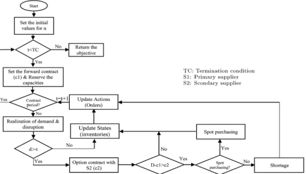
4.1. Simulation procedure
First of all, the simulation procedure is explained. The overall procedure of the simulation is depicted in Figure 3. Note that, in the simulation procedure, Eqs. (4)-(14), dened in Section 3, will be considered. The simulation of the agent-based model is done by an agent-based simulation software package (Netlogo 5.3.1). The optimization part of the SimOpt algorithm is coded in R-studio in cooperation with Netlogo (R-Netlogo), as discussed in Section 4.3.
4.2. Simulation-based estimation
According to Liu et al. [30], we have performed some
analyses on the number of replications of the simula-tion. Indeed, a two-stage decision-making occurs in each time unit (a decision is made before realizing the demand and a decision is made to place an order from reserved supplier and spot market) for each rst stage decision variable; \R" replications are run and the prot function will be calculated based on the results of the replications. In other words, an estimation of the reward function relating to x (i.e., f(x; ")) could be calculated as:
F (xi) = R
P
j=1f(x; "j)
R :
Indeed, in the SimOpt algorithm, the same set of realizations (for demand and all other stochastic pa-rameters) is used in each iteration toward the opti-mization. It was done by using R sets of seeds to generate dierent sequences of stochastic parameters in the replications. In this regard, four sample sizes are dened for the number of replications: 5, 10, 20, 50, and those are labeled with 1-4. Hence, we call four simulation optimization algorithms such as SimOpt-1-4. In the following section, the RL algorithm is described.
4.3. RL algorithm 4.3.1. States
As mentioned before, although the states of the system do not have Markov property, temporal dynamics (or dynamics occurring in each step of the Markov process) make it possible (and give an appropriate approximations) to estimate the reward in the next step based on the current states and actions. States for dierent agents are dened as follows: 1) customer agents: Sc
t, amount of the unsatised demand at time
unit t; 2) retailer agent: Sr
t, the inventory position at
time t; 3) supplier agent: [Sts;1; Sts;2], the remaining
capacity at time t and remaining reserved capacity at time t; and 4) spot market agent: Ssp
t , the inventory
position of the spot market. It is assumed that the capacity of the spot market is innite; thus, the state of the spot market always equals innite. Therefore, system state could be written as follows:
S(t) = [Stc; Str; [Sts;1; Sts;2]; Stsp]:
In order to control the dimension of the above vector, a common approach is used to consider a limited set of cases for each member of the vector, e.g., for Sr
t,
( 1; 1000) 1; [ 1000; 500) 2; :::.
It is worthwhile to note that, in the simulation process (as mentioned in the previous section), xed seeds are used in order to generate random num-bers (especially for sampling from random variables). Hence, in each run of the simulation, the initial conditions will be the same as other runs.
4.3.2. Reward
The reward function at time unit \t" is equivalent to the prot gained by the risk-sensitive retailer at time unit t. Therefore, the reward function can be dened as follows:
rt=pDi;t
X
j
i;tCap2i;jfj
X
j
c1 jxi;j;t
X
j
c2 jyi;j;t
X
t
&i;t !zi;t hIi;t:
In addition, ideally, based on Eq. (2), the Q-function could be obtained. However, since the values of the revenue and costs for the future periods could not be calculated, a Q-learning algorithm is usually used to estimate the value of the function. It is described in the forthcoming sections.
4.3.3. Actions
In the agent-based framework, for each agent, a set of state actions is dened. The states have been explained before. In this section, actions of dierent agents are explained: 1) customer agents: demand based on the normal distribution; 2) retailer agents: orders from suppliers, values of x and y; 3) supplier agents: amount of satised demand by the primary and secondary suppliers; 4) the spot market agent: satised excess demand of the retailer. A customer's demand is dened as a random normal variable. The value of x depends on the risk attitude of the retailer (as explained in Section 3). The value of y is determined by the learning mechanism. The value of the supplier action depends on the constraints explained in Section 3. The value of an action of the spot market is equal to the amount of excess demand requested from the spot market. A decision between shortage and ordering from spot market is determined by the learning mechanism. 4.3.4. Q-learning algorithm
In this section, the proposed Q-learning algorithm is presented to estimate the Q-function. One of the most important challenges of the performance of RL is ecient exploitation and exploration. In the initial steps, more explorations are required and, in further steps, more exploitations must occur. The exploration and exploitation are dened in the Algorithm 1 by parameter .
After taking an action, the system enters a new state. As a result of performing Q-learning algorithm, Q(s; a) matrix is formed for each set of state actions. The convergence of the RL algorithms was surveyed by a wide range of researchers. In the above learn-ing algorithm, is the learnlearn-ing coecient. It is a usual coecient and has a performance like the other similar uses of learning coecients (e.g., the same as the learning coecient in the exponential smoothing forecasting). Indeed, it gives a weight to the old
Algorithm 1. Reinforcement learning.
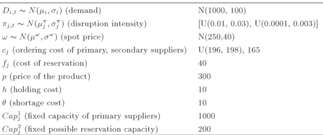
Table 1. Parameters of the model. Di;t N(i; i) (demand) N(1000, 100)
j;t N(j; j) (disruption intensity) [U(0.01, 0.03), U(0.0001, 0.003)]
! N(!; !) (spot price) N(250,40)
cj(ordering cost of primary, secondary suppliers) U(196, 198), 165
fj (cost of reservation) 40
p (price of the product) 300
h (holding cost) 10
(shortage cost) 10
Cap1
j (xed capacity of primary suppliers) 1000
Cap2
j (xed possible reservation capacity) 200
estimations in contrast with the recent results. The stopping criterion of the problem is considered as the maximum iteration.
As shown in Figure 3, the above algorithm is a part of the SimOpt algorithm. Indeed, in each time unit, all the states for the action made at the beginning of the contract period are calculated. At the end of the contract period, the best action is selected and, again, the simulation will run and states are calculated until the next contract period. The procedure will stop whenever the stopping criterion is met. In the next section, a numerical example is solved by using the proposed Q-learning algorithm, and the results are compared with a genetic algorithm-based SimOpt. 5. Numerical example
In this section, the results of implementing the pro-posed Q-learning algorithm are compared with those of another SimOpt algorithm in which Q-learning changes into a common genetic algorithm. Generally, our data from Merzifonluoglu were adopted [1]. Because of some additional assumptions in this paper in contrast with the base paper, some parts of data have been modied. Additional assumptions of our model include multiple
retailers, multiple periods, and time-based disruptions. Details of the numerical example are dened in the Table 1.
Additionally, the probability of disruption is con-sidered as a uniform distribution between [0.01, 0.05]. The disruption eect (or the length of the disruption) is assumed as a uniform distribution between [0, 2] time units. The maximum number of disrupted suppliers is assumed as a uniform distribution between [0, J]. The same as the case of Merzifonluoglu [1], it is assumed that the demand and the spot price are correlated with parameter ( > 0), such that: 1 = ; 2 = !;
11= ; 22= !; 12= 21= !.
The coecient of the correlation is assumed equal to 0.2. Dierent problem instances are dened based on the common NV problem. Problem instances are numbered according to the number of suppliers and retailers. The basic problem instance in this paper is NV10-10, in which the rst number shows the number of suppliers and the second one shows the number of retailers. The number of contract periods and the number of time units in each contract period are 20 and 11, respectively.
Values for , , and by using the simulation were determined as 0.3, 0.2, and 0.4, respectively. Results
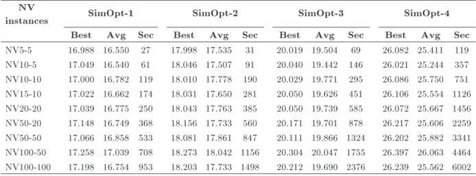
Table 2. Results of the algorithms with dierent replications (106).
NV
instances SimOpt-1 SimOpt-2 SimOpt-3 SimOpt-4
Best Avg Sec Best Avg Sec Best Avg Sec Best Avg Sec
NV5-5 16.988 16.550 27 17.998 17.535 31 20.019 19.504 69 26.082 25.411 119 NV10-5 17.049 16.540 61 18.046 17.507 91 20.040 19.442 146 26.021 25.244 357 NV10-10 17.000 16.782 119 18.010 17.778 190 20.029 19.771 295 26.086 25.750 751 NV15-10 17.022 16.662 174 18.031 17.650 281 20.050 19.626 451 26.106 25.554 1126 NV20-20 17.039 16.775 250 18.043 17.763 385 20.050 19.739 585 26.072 25.667 1456 NV50-20 17.148 16.749 368 18.156 17.733 560 20.171 19.701 878 26.217 25.606 2259 NV50-50 17.066 16.858 533 18.081 17.861 847 20.111 19.866 1324 26.202 25.882 3341 NV100-50 17.258 17.039 708 18.273 18.042 1156 20.304 20.047 1755 26.397 26.063 4464 NV100-100 17.198 16.754 953 18.203 17.733 1498 20.212 19.690 2376 26.239 25.562 6002
Figure 4. The progress of the learning through the SimOpt-3 algorithm (NV10-10-1).
were obtained by a PC with Intel(R) Corei7, 3.1 GHz CPU, and 6 GB RAM.
As discussed in Section 4.2., we have dened four SimOpt algorithms with dierent replication numbers in the simulation procedure. Table 2 shows the results of applying these algorithms on the problem.
Results show that SimOpt-3 is the most proper SimOpt algorithm in terms of accuracy and time. Thus, in the remaining parts of the paper, we only discuss the results given from SimOpt-3.
The result of applying the algorithm (for 100 iterations) to the problem NV10-10-1 is depicted in Figure 4.
As shown in Figure 4, the algorithm converges to a near-optimal prot of the risk-sensitive retailer in 200 iterations. The best prot resulting from applying the algorithm to the problem is 20028766.
To show the eciency of the proposed RL al-gorithm, results are compared with those of another popular metaheuristic based on the simulation pro-cedure. Genetic Algorithm (GA) is a meta-heuristic and evolutionary algorithm that has been used in the literature to optimize many complex problems. It works with some procedures such as mutation and
crossover, originally inspired by genetic science. Re-sults of the SimOpt-RL are compared with those of a simulation-based Genetic Algorithm (SimOpt-GA) applied to the problem. Hence, GA (instead of RL) is used to optimize the simulation procedure explained in Section 4.1. The GA used in this paper is the same as the algorithms used by the related works [2,9,21].
We dened NV10-10-1 as the problem with 10 suppliers and 10 retailers (i.e., 1 risk-sensitive and 9 risk-neutral retailers) where retailers have an option to buy from spot market. The problem NV10-10-2 is dened as a problem in which spot market option is not considered.
In addition, as proposed by Liu et al [30], to show the eciency of the proposed SimOpt-RL algorithm, the results of the SimOpt are compared with a case in which all stochastic parameters are equal to their ex-pected values, called Exex-pected Value Method (EVM). Table 3 shows the comparisons.
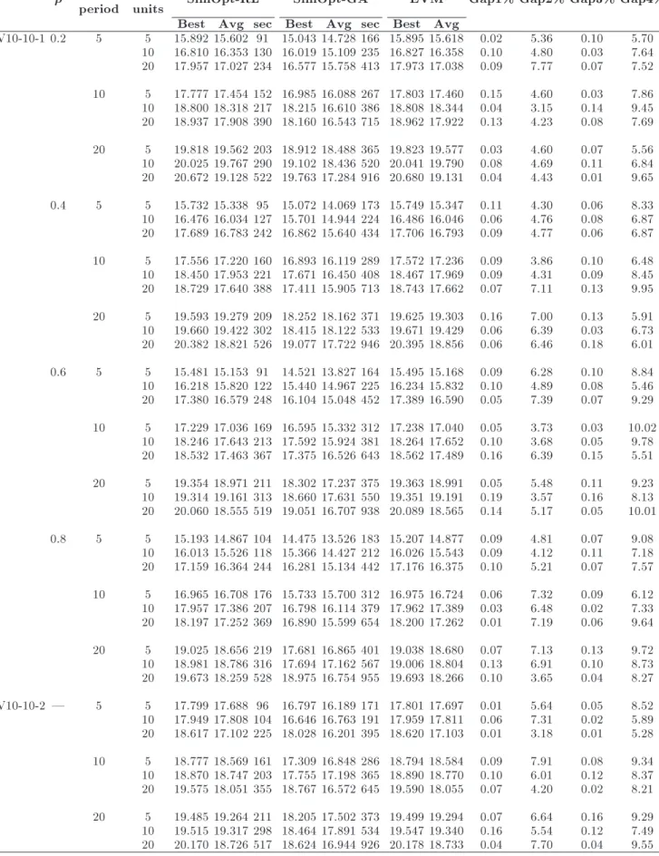
Results show the impact of the correlation (de-creasing), the number of contract periods (increas-ing), and the number of time units (decreasing) on the reward values. Additionally, Gaps #1 and #2 represent the gap between the best values of SimOpt-RL and SimOpt-GA (respectively) with the best value of the EVM. Gaps #3 and #4 show the gap between the average values of SimOpt-RL and SimOpt-GA (respectively) with the average value of EVM. More-over, Table 4 shows the eect of dierent disruption probabilities on the objective function and ll rate (prot values in Tables 4 and 5 are scaled out similar to those in the previous tables).
A sensitivity analysis is done regarding the eect of dierent values for deviation of the parameters: stan-dard deviation of the demand (), stanstan-dard deviation of the disruption eect (), and standard deviation
of the spot price (!). Table 5 shows dierent cases
dened for the sensitivity analysis.
Table 3. A comparison between dierent approaches to solving NV10-10 problem (106).
Contract period
Time
units SimOpt-RL SimOpt-GA EVM Gap1% Gap2% Gap3% Gap4%
Best Avg sec Best Avg sec Best Avg
NV10-10-1 0.2 5 5 15.892 15.602 91 15.043 14.728 166 15.895 15.618 0.02 5.36 0.10 5.70 10 16.810 16.353 130 16.019 15.109 235 16.827 16.358 0.10 4.80 0.03 7.64 20 17.957 17.027 234 16.577 15.758 413 17.973 17.038 0.09 7.77 0.07 7.52 10 5 17.777 17.454 152 16.985 16.088 267 17.803 17.460 0.15 4.60 0.03 7.86 10 18.800 18.318 217 18.215 16.610 386 18.808 18.344 0.04 3.15 0.14 9.45 20 18.937 17.908 390 18.160 16.543 715 18.962 17.922 0.13 4.23 0.08 7.69 20 5 19.818 19.562 203 18.912 18.488 365 19.823 19.577 0.03 4.60 0.07 5.56 10 20.025 19.767 290 19.102 18.436 520 20.041 19.790 0.08 4.69 0.11 6.84 20 20.672 19.128 522 19.763 17.284 916 20.680 19.131 0.04 4.43 0.01 9.65 0.4 5 5 15.732 15.338 95 15.072 14.069 173 15.749 15.347 0.11 4.30 0.06 8.33 10 16.476 16.034 127 15.701 14.944 224 16.486 16.046 0.06 4.76 0.08 6.87 20 17.689 16.783 242 16.862 15.640 434 17.706 16.793 0.09 4.77 0.06 6.87 10 5 17.556 17.220 160 16.893 16.119 289 17.572 17.236 0.09 3.86 0.10 6.48 10 18.450 17.953 221 17.671 16.450 408 18.467 17.969 0.09 4.31 0.09 8.45 20 18.729 17.640 388 17.411 15.905 713 18.743 17.662 0.07 7.11 0.13 9.95 20 5 19.593 19.279 209 18.252 18.162 371 19.625 19.303 0.16 7.00 0.13 5.91 10 19.660 19.422 302 18.415 18.122 533 19.671 19.429 0.06 6.39 0.03 6.73 20 20.382 18.821 526 19.077 17.722 946 20.395 18.856 0.06 6.46 0.18 6.01 0.6 5 5 15.481 15.153 91 14.521 13.827 164 15.495 15.168 0.09 6.28 0.10 8.84 10 16.218 15.820 122 15.440 14.967 225 16.234 15.832 0.10 4.89 0.08 5.46 20 17.380 16.579 248 16.104 15.048 452 17.389 16.590 0.05 7.39 0.07 9.29 10 5 17.229 17.036 169 16.595 15.332 312 17.238 17.040 0.05 3.73 0.03 10.02 10 18.246 17.643 213 17.592 15.924 381 18.264 17.652 0.10 3.68 0.05 9.78 20 18.532 17.463 367 17.375 16.526 643 18.562 17.489 0.16 6.39 0.15 5.51 20 5 19.354 18.971 211 18.302 17.237 375 19.363 18.991 0.05 5.48 0.11 9.23 10 19.314 19.161 313 18.660 17.631 550 19.351 19.191 0.19 3.57 0.16 8.13 20 20.060 18.555 519 19.051 16.707 938 20.089 18.565 0.14 5.17 0.05 10.01 0.8 5 5 15.193 14.867 104 14.475 13.526 183 15.207 14.877 0.09 4.81 0.07 9.08 10 16.013 15.526 118 15.366 14.427 212 16.026 15.543 0.09 4.12 0.11 7.18 20 17.159 16.364 244 16.281 15.134 442 17.176 16.375 0.10 5.21 0.07 7.57 10 5 16.965 16.708 176 15.733 15.700 312 16.975 16.724 0.06 7.32 0.09 6.12 10 17.957 17.386 207 16.798 16.114 379 17.962 17.389 0.03 6.48 0.02 7.33 20 18.197 17.252 369 16.890 15.599 654 18.200 17.262 0.01 7.19 0.06 9.64 20 5 19.025 18.656 219 17.681 16.865 401 19.038 18.680 0.07 7.13 0.13 9.72 10 18.981 18.786 316 17.694 17.162 567 19.006 18.804 0.13 6.91 0.10 8.73 20 19.673 18.259 528 18.975 16.754 955 19.693 18.266 0.10 3.65 0.04 8.27 NV10-10-2 | 5 5 17.799 17.688 96 16.797 16.189 171 17.801 17.697 0.01 5.64 0.05 8.52 10 17.949 17.808 104 16.646 16.763 191 17.959 17.811 0.06 7.31 0.02 5.89 20 18.617 17.102 225 18.028 16.201 395 18.620 17.103 0.01 3.18 0.01 5.28 10 5 18.777 18.569 161 17.309 16.848 286 18.794 18.584 0.09 7.91 0.08 9.34 10 18.870 18.747 203 17.755 17.198 365 18.890 18.770 0.10 6.01 0.12 8.37 20 19.575 18.051 355 18.767 16.572 645 19.590 18.055 0.07 4.20 0.02 8.21 20 5 19.485 19.264 211 18.205 17.502 373 19.499 19.294 0.07 6.64 0.16 9.29 10 19.515 19.317 298 18.464 17.891 534 19.547 19.340 0.16 5.54 0.12 7.49 20 20.170 18.726 517 18.624 16.944 926 20.178 18.733 0.04 7.70 0.04 9.55
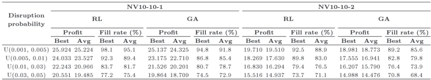
Table 4. Sensitivity analysis of dierent disruption probabilities.
NV10-10-1 NV10-10-2
Disruption
probability RL GA RL GA
Prot Fill rate (%) Prot Fill rate (%) Prot Fill rate (%) Prot Fill rate (%) Best Avg Best Avg Best Avg Best Avg Best Avg Best Avg Best Avg Best Avg U(0.001, 0.005) 25.924 25.224 98.1 95.1 25.137 24.325 94.8 91.8 19.710 19.510 92.5 88.9 18.981 18.773 89.2 85.6 U(0.005, 0.01) 24.033 23.527 92.3 89.4 23.175 22.710 86.8 85.4 18.269 17.630 89.8 83.0 17.555 16.941 82.8 79.8 U(0.01, 0.03) 22.243 20.966 83.7 81.7 21.526 20.201 80.7 78.7 16.830 16.294 79.4 76.5 16.207 15.790 76.4 73.9 U(0.03, 0.05) 20.551 19.485 77.2 75.4 19.864 18.709 74.5 72.9 15.516 14.937 73.7 71.1 14.988 14.476 70.8 68.4
Table 5. Dierent cases of sensitivity analysis.
Lower Low High Higher
10 50 150 250
U(0.0001, 0.0005) U(0.0005, 0.001) U(0.003, 0.005) U(0.005, 0.01)
! 10 25 50 60
Table 6. Sensitivity results of , , and !.
NV10-10-1 NV10-10-2
RL GA RL GA
Prot Fill rate (%) Prot Fill rate (%) Prot Fill rate (%) Prot Fill rate (%) Best Avg Best Avg Best Avg Best Avg Best Avg Best Avg Best Avg Best Avg Lower 23.105 22.852 98.9 95.7 22.342 22.156 95.9 92.0 22.619 22.346 93.5 89.7 21.920 21.510 89.8 86.6 Low 21.538 21.427 97.9 94.9 20.876 20.691 94.7 91.1 21.005 20.854 92.5 88.6 20.311 20.212 88.9 85.5 High 18.374 18.165 95.6 93.4 17.809 17.455 92.0 90.5 17.905 17.691 91.0 86.9 17.284 17.095 87.7 84.3 Higher 16.996 16.627 95.9 92.6 16.338 15.974 92.7 89.7 16.445 16.360 90.6 86.3 15.800 15.717 87.3 83.4 Lower 21.582 21.378 97.6 94.5 20.892 20.552 94.2 91.0 21.071 20.918 92.8 88.8 20.389 20.134 89.9 85.5
Low 20.896 20.629 97.5 94.7 20.266 19.880 93.9 90.9 20.436 20.233 92.4 88.6 19.691 19.566 89.2 85.7 High 19.082 18.875 95.9 93.6 18.468 18.163 92.7 90.0 18.754 18.441 91.1 87.0 18.106 17.744 87.5 83.8 Higher 18.509 18.183 96.7 93.5 17.861 17.528 93.3 89.9 18.000 17.714 90.7 86.8 17.451 17.019 87.6 83.5 ! Lower 22.033 21.898 97.7 95.0 21.338 21.153 94.0 91.5 - - - - - - -
-Low 21.055 20.922 97.5 95.0 20.355 20.210 94.3 91.5 - - - -High 18.947 18.608 95.8 93.0 18.232 17.911 92.3 90.1 - - - -Higher 17.871 17.704 96.2 93.5 17.222 17.016 92.7 90.6 - - -
-values for the mentioned cases. Results show the decreasing eect of the wider deviations on the values of the prot and ll rate.
In the remaining part of this section, the resulted risk behavior of the risk-sensitive retailer is discussed according to the best solution obtained.
Figure 5 shows the accumulated prot during 20 contract periods of the best solutions of two algorithms in NV10-10-1 problem.
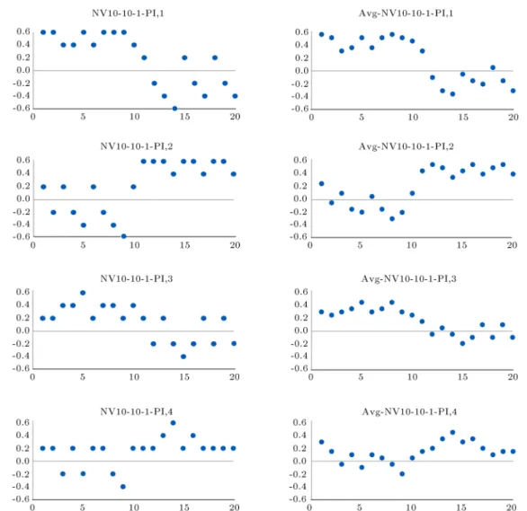
Based on the analyses presented in Tables 3, 4, and 6 and Figures 4 and 5, the eciency of the proposed SimOpt-RL algorithm is shown. Therefore, in the remaining part of this section, the detailed results of the RL algorithm in dierent cases of the NV10-10-1 are discussed. Based on the cases introduced in this section, the following NV10-10-1 problem in-stances (NV10-10-1-PI) are considered, as shown in Table 7.
Figure 6 shows the results of the best and average
Figure 5. Comparison of the best solutions of RL and GA SimOpt algorithm regarding accumulated rewards in NV10-10-1.
solutions of the SimOpt-RL for these four problem instances.
According to the results shown in Figure 6, it could be concluded that decisions related to the risk attitude of the risk-sensitive retailer have an important
Table 7. Dierent problem instances of NV10-10-1 problem.
NV10-10-1-PI,1 NV10-10-1-PI,2 NV10-10-1-PI,3 NV10-10-1-PI,4
Contract periods 1-10 Higher Higher Lower Lower Higher Lower Lower Higher Contract periods 11-20 Lower Lower Higher Higher Lower Higher Higher Lower
Figure 6. Risk attitude of the risk-sensitive retailer in the best (left) and average (right) solutions of the SimOpt-RL in dierent problem instances.
impact on the prot (reward) function. Additionally, more deviations of the demand and disruption intensity result in more risk-averse behavior. Furthermore, demand deviation has a greater eect on the risk averseness of the retailer rather than disruption in-tensity deviation. In the rst two cases with high demand deviations, the retailer shows an extremely risk-averse behavioral pattern in approximately 30% of the times, while, in the last two cases with lower demand deviations, the retailer is extremely risk averse in 5% of the times. Extreme risk-taking behavior is only obtained by the lower demand and disruption deviations. These results could help a decision-maker
in an uncertain environment (on both sides of the supply chain) to make a decision with an acceptable average reward.
6. Conclusions
The importance of decision-making in an uncertain supply chain has led researchers to develop intelligent approaches to solve complex problems in an ecient manner. The NV problem is a popular problem that has been extended in many dierent ways in the past years. However, in recent years, the NV problem with multiple unreliable suppliers is a type of problem
that has received much attention [1-3,12-14]. The complexity of the obtained problem has forced the researchers to adopt heuristic or intelligent approaches. The main idea of our model was derived initially from previously mentioned works. A conguration proposed by Merzifonluoglu [1] consists of one retailer and many suppliers that are subjected to disruptions. In this con-guration, retailers sign forward and option contracts before demand realization and can buy products from the spot market after the realization. These options are common in industries such as semiconductors, telecom-munications, and pharmaceuticals. In this paper, a new model was developed based on this conguration. In addition to demand uncertainty and supplier disrup-tions, a multi-period, multi-agent model with many-to-many relations between risk-sensitive retailers and capacitated suppliers was developed. Further, an RL method (as an optimization approach) was presented to solve it. Dierent simulation congurations (with dierent numbers of realization) were examined on dierent scales of the problem. Results showed an acceptable performance of the SimOpt algorithm in contrast with the non-stochastic algorithm. Moreover, results of the SimOpt-RL were compared with those of a SimOpt algorithm based on the genetic algorithm. Several sensitivity analyses were carried out regarding dierent parameters (including the number of contract periods, the number of time units in each contract period, standard deviations of demands, and disrup-tions). Moreover, details of the decisions were obtained based on a sample problem (NV10-10-1). For the future studies, considering multiple products in the problem would be an interesting idea and a more challenging design. In addition, considering negotiation process and transportation assumptions is another suggestion in order to extend the work presented in this paper. Nomenclature
NV Newsvendor
NVP Newsvendor Problem
NVPSD Newsvendor Problem with
Supplier Disruption
MNVPSD Multi-period Newsvendor
Problem with Supplier Disruption
ABMS Agent-Based Modeling and
Simulation
RL Reinforcement Learning
SimOpt Simulation Optimization
SimOpt-RL Simulation Optimization based on Reinforcement Learning
SimOpt-GA Simulation Optimization based on Genetic Algorithm SimOpt X Simulation Optimization
approach with 5, 10, 20, 50
replications in each simulation run, X 2 f1; 2; 3; 4g
NV10-10-1 A newsvendor problem with 10
suppliers and 10 retailers (i.e. 1 risk-sensitive and 9 risk-neutral retailers) in which retailers have an option to buy from the spot market
NV10-10-2 A newsvendor problem with 10
suppliers and 10 retailers (i.e. 1 risk-sensitive and 9 risk-neutral retailers) in which the spot market option is neglected
NV10-10-1 -PI, X
Dierent problem instances dened based on the NV10-10-1, X 2 f1; 2; 3; 4g
EVM Expected Value Method
References
1. Merzifonluoglu, Y. \Risk averse supply portfolio selec-tion with supply, demand and spot market volatility", Omega, 57, pp. 40-53 (2015).
2. Ray, P. and Jenamani, M. \sourcing under supply dis-ruption with capacity-constrained suppliers", Journal of Advances in Management Research, 10(2), pp. 192-205 (2013).
3. Ray, P. and Jenamani, M. \sourcing decision under disruption risk with supply and demand uncertainty: A newsvendor approach", Annals of Operations Re-search, 237(1), pp. 237-262 (2016).
4. Kim, G., Wu, K., and Huang, E. \Optimal inventory control in a multi-period newsvendor problem with non-stationary demand", Advanced Engineering Infor-matics, 29(1), pp. 139-145 (2015).
5. Chopra, S. and Meidl, P., Supply Chain Management: Strategy, Planning and Operation, Pearson, Sixth edi-tion, USA (2016).
6. Chiacchio, F., Pennisi, M., Russo, G., Motta, S., and Pappalardo, F. \Agent-based modeling of the immune system: NetLogo, a promising framework", BioMed Research International, 2, pp. 1-6 (2014).
7. Humann, J. and Madni, A.M. \Integrated agent-based modeling and optimization in complex systems analysis", Procedia Computer Science, 28, pp. 818-827 (2014).
8. Macal, C.M. \Everything you need to know about agent-based modelling and simulation", Journal of Simulation, 10, pp. 144-156 (2016).
9. Avci, M.G. and Selim, H. \A multi-objective, simulation-based optimization framework for supply
chains with premium freights", Expert Systems with Applications, 67, pp. 95-106 (2017).
10. Sutton, R.S. and Barto, A.G., Reinforcement Learning: An Introduction, MIT press, Cambridge (1998).
11. Gosavi, A. \Reinforcement learning for long-run aver-age cost", European Journal of Operational Research, 155, pp. 654-674 (2004).
12. Merzifonluoglu, Y. and Feng, Y. \Newsvendor prob-lem with multiple unreliable suppliers", International Journal of Production Research, 52(1), pp. 221-242 (2014).
13. Merzifonluoglu, Y. \Impact of risk aversion and backup supplier on sourcing decisions of a rm", International Journal of Production Research, 53(22), pp. 6937-6961 (2015).
14. Merzifonluoglu, Y. \Integrated demand and procure-ment portfolio manageprocure-ment with spot market volatility and option contracts", European Journal of Opera-tional Research, 258(1), pp. 181-192 (2017).
15. Bouakiz, M. and Sobel, M.J. \Inventory control with an exponential utility criterion", Operations Research, 40(3), pp. 603-608 (1992).
16. Wang, H.F., Chen, B.C., and Yan, H.M. \Optimal inventory decisions in a multi period newsvendor problem with partially observed Markovian supply capacities", European Journal of Operational Research, 202, pp. 502-517 (2010).
17. Densing, M. \Dispatch planning using newsvendor dual problems and occupation times: application to hydropower", European Journal of Operational Re-search, 228, pp. 321-330 (2013).
18. Jalali, H. and Nieuwenhuyse, I.V. \Simulation opti-mization in inventory replenishment: a classication", IIE Transactions, 47, pp. 1217-1235 (2015).
19. Nikolopoulou, A. and Ierapetritou, M.G. \Hybrid sim-ulation based optimization approach for supply chain management", Computers & Chemical Engineering, 47, pp. 183-193 (2012).
20. Kwon, O., Im, G.P., and Lee, K.C. \MACE-SCM: A multi-agent and case-based reasoning collaboration mechanism for supply chain management under sup-ply and demand uncertainties", Expert Systems with Applications, 33(3), pp. 690-705 (2007).
21. Chaharsooghi, S.K., Heydari, J., and Zegordi, S.H. \A reinforcement learning model for supply chain ordering management: An application to the beer game", Decision Support Systems, 45(4), pp. 949-959 (2008).
22. Sun, R. and Zhao, G. \Analyses about eciency of reinforcement learning to supply chain ordering management", IEEE 10th International Conference on Industrial Informatics, China (2012).
23. Dogan, I. and Guner, A.R. \A reinforcement learning approach to competitive ordering and pricing prob-lem", Expert Systems, 32(1), pp. 39-48 (2015).
24. Jiang, C. and Sheng, Z. \Case-based reinforcement learning for dynamic inventory control in a multi-agent supply-chain system", Expert Systems with Applica-tions, 36(3), pp. 6520-6526 (2009).
25. Kim, C.O., Kwon, I.-H., and Kwak, C. \Multi-agent based distributed inventory control model", Ex-pert Systems with Applications, 37(7), pp. 5186-5191 (2010).
26. Mortazavi, A., Khamseh, A.A., and Azimi, P. \De-signing of an intelligent self-adaptive model for sup-ply chain ordering management system", Engineering Applications of Articial Intelligence, 37, pp. 207-220 (2015).
27. Rabe, M. and Dross, F. \A reinforcement learning approach for a decision support system for logis-tics networks", Winter Simulation Conference, USA (2015).
28. Zhou, J., Purvis, M., and Muhammad, Y. \A com-bined modelling approach for multi-agent collaborative planning in global supply chains", 8th International Symposium on Computational Intelligence and Design, China (2015).
29. Thiele, J. and Marries, R. \NetLogo: introduction to the RNetLogo package", Journal of Statistical Soft-ware, 58, pp. 1-41 (2014).
30. Liu, R., Tao, Y., Hu, Q., and Xie, X. \Simulation-based optimisation approach for the stochastic two-echelon logistics problem", International Journal of Production Research, 55(1), pp. 187-201 (2017).
Biographies
Abdollah Aghaie is a Professor of Industrial En-gineering at K.N. Toosi University of Technology in Tehran, Iran. He received his BSc from Sharif University of Technology in Tehran, MSc from New South Wales University in Sydney, and PhD from Loughborough University in U.K. His main research interests lie in modeling and simulation, supply chain management, social networks, knowledge management, and risk management.
Mojtaba Hajian Heidary is a PhD student of Industrial Engineering at K.N. Toosi University of Technology, Department of Industrial Engineering, Tehran, Iran. His main research interests are supply chain management and computer simulation.