Abstract
Recent work has suggested that parts of the Appalachian Mountains were uplifted during the Neogene, based on stream knickpoint analysis (Gallen et al., 2013; Miller et al., 2013). Analysis of the symmetry of valleys has the potential to indicate tectonic activity by determining migration trends of channels. Tectonic quiescence promotes lateral migration of stream bends. This creates asymmetrical bend valleys with shallow point bars and steep cut banks. Uplift promotes downcutting over lateral migration, producing symmetrical stream valleys. Using LIDAR data and ArcMap software, I quantified the symmetry of stream valleys in the Blue Ridge Mountains of western North Carolina. I calculated the symmetry of valleys by dividing the right valley slope by the left valley slope to form ratios ranging from 0 to 1, with 1 indicative of a symmetrical valley. Where the right slope exceeded the left slope, I inverted the ratio to avoid numbers greater than 1. I measured slope ratios across the Broad, Cullasaja, French Broad, Linville, New, Pigeon, Toe, and Tuckasegee Rivers. To separate similar symmetry values between areas of gentle and steep topography, I multiplied the symmetry value by the average of the right and left slopes. The resultant values were then combined with a knickpoint propagation model to project areas of equilibrating streams and relict
Introduction
The morphology of rivers, particularly river profiles, exerts control over topography in landscapes undergoing erosion (Kirby and Whipple, 2012). Workers have implemented numerous methods to detect active landscapes undergoing response to uplift, many of which involve analyzing river profiles. Typical channels respond to increased uplift rates by steepening longitudinal profile gradients, which results in the creation and upstream propagation of knickpoints (Whipple and Tucker, 1999). Knickpoint analysis is commonly employed to locate equilibrating streams, and may also be used to estimate changes in relief (Gallen et al., 2013; Miller et al., 2013). Areas containing knickpoints may be located using the normalized steepness calculation !=!!"!!!"#$, which can
highlight channel slopes that exceed the expected steepness for their given drainage areas (Wobus et al., 2006).
Unlike the broad valleys of laterally migrating rivers, incised valleys often host steep, symmetrical walls that exhibit downcutting. Such downcutting is a result of ongoing equilibration to uplift, and areas with incised valleys often contain knickpoints
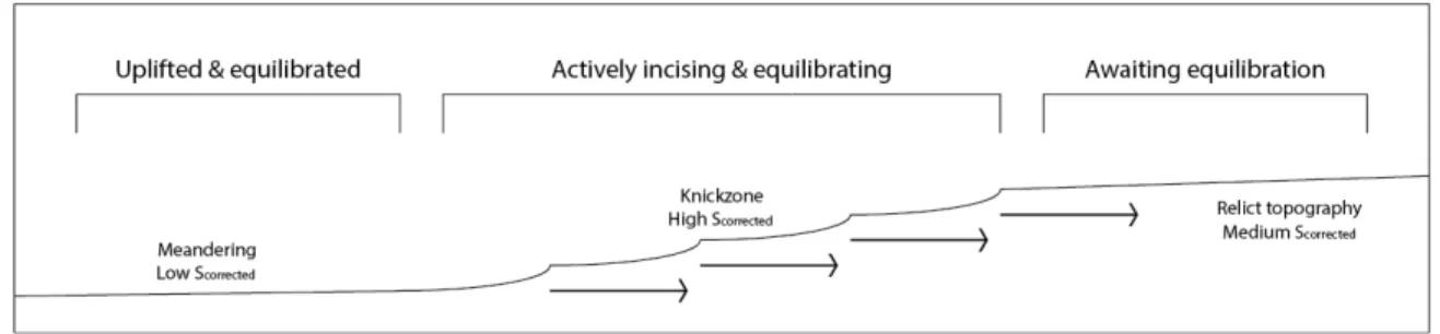
throughout their reaches. Downstream of the incised area, already equilibrated valleys gradually begin to meander and broaden. The longitudinal anatomy of an equilibrating stream is illustrated in Figure 1. The study used the calculated symmetry of valleys to digitally locate potential areas of incision. Valley symmetry was then applied to the aforementioned knickpoint propagation model to estimate locations that may be responding to Neogene uplift.
Study Area
The investigation focused on North Carolina’s Blue Ridge Mountains, as shown in Figure 2. Eight rivers evenly distributed across the field area were included in the study. Small streams were avoided, and instead I focused upon well-established channels. The French Broad River was chosen for its extent, which reaches from Transylvania County
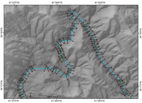
northward into Tennessee. The Cullasaja River had been previously investigated by Gallen et al. (2013) and was selected for its extensive documentation that greatly aided in interpretations. As it had already been hypothesized as an active landscape, I used its valley morphology sequences to project additional locations of potentially active
included in the distribution and scatter plot of corrected symmetry due to its potential fractures, but was nonetheless a channel of interest.
It should be noted that rivers flowing through the mountains of North Carolina are not isolated; to the contrary, they are often chosen as prime locations for homes and roads. The French Broad River flows through heavily populated areas, and the Pigeon River valley hosts an interstate near the North Carolina – Tennessee border. Another common occurrence is the construction of dams and lakes, which affect multiple rivers in the area (namely, the Pigeon and Tuckasegee Rivers). Anthropogenic interference has likely hindered the accuracy of the project’s data to some extent, as have natural features such as unaccounted for mass-wasting events. Future expansions of the study would ideally focus on low-population areas with minimal human development and slope failure.
Methods
the channel multiple times (a frequent occurrence in very low-radius meanders). I recorded elevations at each transect’s vertices and midpoint, and used them to calculate slopes for each side of the valley using the following equations:
m!"#$%= !!"#$%!!!"##$%
!"" & m!"#$ =
!!"#$!!!"##$%
!""
I determined the symmetry (S) of each transect by dividing the right slope by the left slope. In instances where the right slope exceeded the left slope and S>1, the ratio was inverted. The end result was a number between 0 and 1 that still reflected deviation from absolute symmetry, where S=1.
S=mm!"#$% !"#$ =
Z!"#$%−Z!"##$% 100
100
Z!"#$−Z!"##$% =
Z!"#$%−Z!"##$%
Z!"#$−Z!"##$%
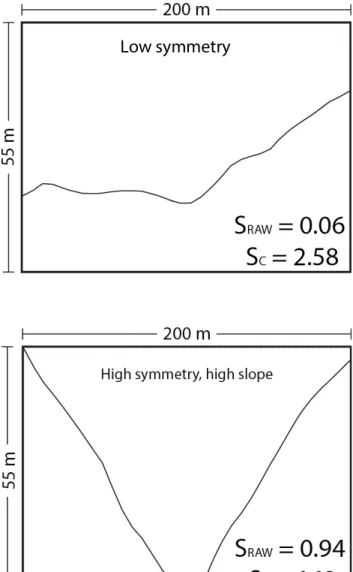
The resultant S-value calculated valley symmetry but was unable to distinguish between symmetrical valleys in broad floodplains and those in narrow, V-shaped valleys (Figure 4). To facilitate the detection of high-symmetry, high-slope areas, I multiplied the
symmetry value by the average of the two slopes. The formula resulted in high values for areas of potential incision, and low values for broad, flat floodplains. I designated these values as “corrected symmetry,” and used them for all interpretations and figures.
S! = Z!"#$%−Z!"##$% Z!"#$ −Z!"##$%
Z!"#$%+Z!"#!
2 −Z!"##$%
Results
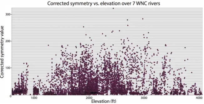
Corrected symmetry values exhibited wide variations and often changed dramatically along rivers (compare Figures 6 and 7 of the Linville River). Few rivers hosted high corrected symmetry values, as evidenced in Figure 8. The majority of valleys were asymmetrical and contained gentle slopes, which implies that incision is a comparatively rare event in the study area. I plotted corrected symmetry values against elevation and found no linear trend between the two. It should be noted that maximum corrected symmetry values are located at intermediate elevations, somewhere between 460-1040 meters (Figure 9). This could be attributed to the model of equilibrating streams linking equilibrated areas to relict topography, as discussed in Figure 1.
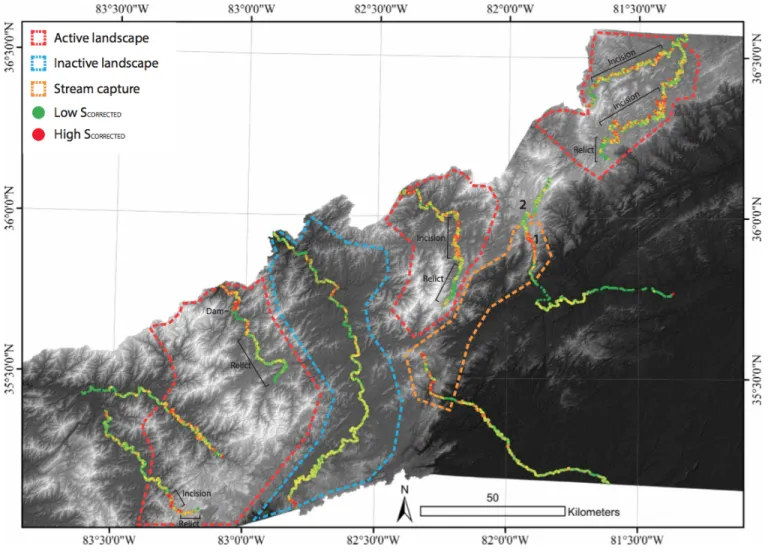
Extended areas of incision were uncommon occurrences, but nevertheless appeared in expected patterns. The Cullasaja River adhered closely to the model of equilibrating streams, as illustrated in Figure 10. At high elevations, relict topography appeared with low-to-medium corrected symmetry values. Such values indicate moderate incision with varying degrees of symmetry, which vary intermediately throughout the stretch of river. At intermediate elevations the river becomes markedly more incised, suggesting that the area is undergoing downcutting and equilibration. The DEM also shows that the
surrounding topography becomes considerably more rugged, which could be further illustrated with a map of local relief. Corrected symmetry past the area of incision drops below previous values, which indicates a greater level of lateral migration and
exhibited by the Cullasaja River was employed to decipher corrected symmetry patterns throughout the field area and indicate areas of active landscape (Figure 5).
Conclusions
Figure 1. I used the above model to characterize active landscapes. Streams flowing through uplifted areas undergo equilibration, which is often marked by knickpoints and high-energy flow. Such areas also host vertically incising streams, while already-equilibrated stream segments at lower elevations exhibit broad, asymmetrical valleys. Uplifted areas are higher elevations that have not yet been affected by upstream
knickpoint propagation host relict topography and low-to-moderate corrected symmetry.
Figure 4a. This cross-section exhibits low raw symmetry and moderate average slope. It appears to be laterally migrating, as evidenced by the steep cut bank and gently sloping point bar. The low raw symmetry and moderate average slope produce a low corrected symmetry value.
Figure 4b. This cross-section shows very high raw symmetry and high average slope. It appears to be vertically incising, with little to no lateral migration. The high raw symmetry and high average slope produce a high corrected symmetry value.
Figure 4c. This cross section exhibits high raw symmetry, which is
misleading given the broad flood plain in which the channel flows. The low average slope corrects for the high raw symmetry and results in a low corrected symmetry
! !
! !
! !
! !
Figure 8. The distribution of corrected symmetry values was heavily skewed, indicating that instances of highly symmetrical and steep-sloping valleys were uncommon. Instead, the majority of streams flow through broad valleys and experience lateral migration.
! !
! !
References Cited
Crosby, B.T., and Whipple, K.X., 2006, Knickpoint initiation and distribution within fluvial networks: 236 waterfalls in the Waipaoa River, North Island, New Zealand: Geomorphology, v. 82, no. 1–2, p. 16–38.
Ferreira, Mateus, 2014. Transect tool for ArcGIS 10.1 available online at http://gis4geomorphology.com/stream-transects-partial/
Gallen, S.F., Wegmann, K.W., Bohnenstiehl, D.R., 2013. Miocene rejuvenation of topographic relief in the southern Appalachians. GSA Today 23, 4–10.
Miller, S., Sak, P., Kirby, E., & Bierman, P. Neogene rejuvenation of central Appalachian topography: Evidence for differential rock uplift from stream profiles and erosion rates. Earth and Planetary Science Letters, , 1-12.
Ritter, D. F., Kochel, R. C., & Miller, J. R. (2011). Process geomorphology (5th ed.). Long Grove, Ill.: Waveland Press.
Whipple, K.X., Tucker, G.E., 1999. Dynamics of the stream-power river incision model: implications for height limits of mountain ranges, landscape response timescales, and research needs. J. Geophys. Res. 104, 17661–17674.
! !
Appendix : Creating maps of corrected symmetry
First download the tools and elevation models necessary to calculate the symmetry of
stream valleys. I used LIDAR files available from the North Carolina Department of
Transportation at https://connect.ncdot.gov/resources/gis/pages/cont-elev_v2.aspx. I also
employed a free transect tool available at
http://gis4geomorphology.com/stream-transects-partial. This tutorial will assume the user is employing the above transect tool.
Use DEM file to create fill, flow direction, and flow accumulation rasters. These layer
files will be used to calculate locations of streams, which will form the basis of the
analysis. The fill raster will eliminate sinks and imperfections, which could impede the
creation of stream paths. Depending on the quality of the DEM raster being used,
multiple fills may be required to adequately smooth the terrain and remove sinks. The
flow direction raster determines which directions water will flow, and will be used in
calculating the flow accumulation raster. The flow accumulation raster illustrates the
drainage area of any given point, which is useful for locating channels.
Now I will create the stream path to be analyzed. First, locate the headwaters of the
channel of interest. Once a starting location is pinpointed, create a shapefile by opening
the project’s folder and clicking File>>New>>Shapefile. Ensure that the shapefile has
the same projection as the basemap- if the two are different projections, compatibility
issues may arise. Once the shapefile is added, right-click the shapefile and navigate to
Editor>>Start editing. Use the tool to add a point where the channel path should start,
! !
Tools>>Distance>>Cost Path. Use the following parameters as inputs to create a stream
path raster:
-Input raster = shapefile
-Destination field = Id
-Cost distance raster = flow accumulation raster
-Cost backlink raster = flow direction raster
-Path type = EACH_CELL
The process of creating a cost path raster may take several minutes depending on the
channel length, DEM quality, and available processing power. Once the raster is done, it
must be converted to a polyline feature that is compatible with the tool. To create a
polyline, navigate to ArcToolbox>>Conversion Tools>>From Raster>>Raster to Polyline
and use the following parameters:
-Input raster = cost path raster
-Field = do not change
-Background value = ZERO
-Minimum dangle length = 0
-Simplify polylines = yes
Now that a stream path polyline is available, it is time to create transects for analyzing
! !
transects at vertices.” The approximate intervals method, while promising a more
consistent transect distribution, is prone to errors. Next, choose an appropriate length for
the transects. I used transects that extended 100 meters from the stream on both sides,
but varying topography may call for different transect parameters. Run the tool.
A fraction of the transects will be incomplete, and will not extend across both sides of the
channel. To erase the incomplete transects, find those with different lengths than the
complete transects and erase them by following the instructions below:
-Right click the transect layer and navigate to the attribute table
-Right-click the field heading for which you want to make a calculation and
click Calculate Geometry.
-Click the geometric property you want to calculate. In this case, it is length.
-Confirm the choice and append the calculations.
-Sort the lengths and note which lengths correspond to incomplete transects. Begin
editing the layer, and delete the incomplete transects. Save the edits, but do not yet stop
editing.
Once the incomplete transects have been eliminated, delete the start and end transects.
They can cause problems when separating the sides of the stream. There may also be
transects that cross the stream twice. They must be eliminated, or unwanted datapoints
will be created later in the process. To eliminate double-crossing transects, simply
! !
times. Stop editing and save. Problematic transects are common in particularly
low-radius meanders, but may also be found in straight areas thanks to the nature of the
transect tool. It is absolutely essential to remove all transects that cross the stream twice,
or future work will be for naught.
Now it is time to create the datapoints that will serve as the sample areas for the
symmetry values. The datapoints will be assigned elevations and used to calculate
symmetry. To plot the points, follow the instructions below. The first step generates the
transect endpoints (Z1 and Z3) and the second generates the transect midpoints (Z2).
-Run Data Management Tools>>Features>>Feature Vertices to Points
-Input features = transects
-Point type = BOTH ENDS
-Run Geoprocessing>>Intersect
-Input features = stream polyline, transects
-JoinAttributes = ALL
-Output type = POINT
The transect endpoints must be separated into right-side and left-side sets. To do so,
create a buffer that encompasses all transects on the right side. It will be used to select all
! !
-Run Analysis Tools>>Proximity>>Buffer
-Input features = polyline
-Distance
-Linear unit = distance greater than transect length
-Side type = right
-End type = flat
-Dissolve type = none
-Run Selection>>Select by Location
-Selection method = select features from
-Target layers = transect vertices
-Source layer = right side buffer
-Spatial selection method = are completely within the source layer feature
-Extract vertices for each side
-Right-click layer containing highlighted transect vertices>>data>>export data
-Output feature class = shapefile
To obtain vertices for the left side, go to the attribute table of all vertices and reverse
selection, then repeat the data export process. You should now have sets of right-side
and left-side points, the lengths of which must be the same. The lengths of the sets also
! !
probably due to an incomplete transect or a double-crossing transect. If all lengths
coincide, proceed to the next step.
I must convert the midpoint set to a file type that can accept elevation and location data.
The step below converts it from a multipart file type into a singlepart file type, similar to
the left-side and right-side datasets:
-Turn intersect point file from multipart file type into singlepart file type
-Use data management>>multipart to singlepart
-Input = intersects
I now have three point files which represent the endpoints and midpoints of the transects.
I just need to give them elevation data, and they will be ready for analysis. Once that's
done, I'll add XY (location) data to the midpoint set and use that information to plot the
calculated symmetry. The two following steps append elevation data to all three point
files and location data to the midpoint file.
-Run Spatial Analyst>>Extraction>>Extract Values to Points
-Input point features = point file
-Input raster = DEM
-Repeat for all three point files
! !
-Input features = midpoint set file
Now I need to associate the individual points with each other. Since points lie on the
same transect, I can use the join feature to apply the transect FID to each point. Later, I
will use the ID to associate all the points from different files. To append transect IDs:
-Right-click point layer>>Joins and Relates>>Join
-Join data from another layer based on spatial location
-Layer to join = transect polyline layer
-You are joining: lines to points
-Each point will be given all attributes of the line that is closest...
-Save as = rightjoin.shp ,leftjoin.shp , midjoin.shp
At this point, all work in ArcMap is complete. The files must be exported as databases,
also known as .dbf or dBASE tables, and analyzed in a spreadsheet program. Repeat the
process below for all three point files.
-Attribute table>>Table Options>>Export
-Export = All records
-Output table = y1.dbf , y2.dbf ,y3.dbf
! !
Open the files in the spreadsheet program of your choice. Microsoft Excel or OpenOffice
Calc will both perform the necessary calculations.
-Order y1,y2,y3 sheets by ascending FID_2.
-Copy y1, y2, and y3 RASTERVALUE (elevation) columns into a new working
spreadsheet and ensure that they are in adjacent columns.
-Create new column titled “raw” in the working spreadsheet with the equation
=ABS((y1-y2)/(y3-y2)). This will render the raw symmetry information. Some still exceed 1, which
is easily fixed.
-Create new column titled “fixed” in the working spreadsheet and use the IF() function to
ignore values less than 1 and invert values greater than 1. The final product should have
no values greater than 1.
-Create a new column in the working spreadsheet that subtracts the middle elevation (y2)
from the average surrounding elevation ((y1+y3)/2). Use the formula (y1+y3)/2-y2. This
is the “multiplier.” Multiply the “fixed” values by this number in a new column to obtain
the corrected symmetry.
-Open a final spreadsheet and paste XY data from mid-transect points into the first two
! !
column, paste the “fixed” values. In the fourth column, paste the “multiplier.” In the
fifth column, paste the corrected symmetry.
-Save the spreadsheet as a .dbf file.
-Open up ArcMap, then go to File>>Add Data>>Add XY Data
-Set the corrected symmetry column as the Z value, and adjust symbology to reflect