TECHNICAL UNIVERSITY OF CLUJ-NAPOCA
ACTA TECHNICA NAPOCENSIS
Series: Applied Mathematics, Mechanics and Engineering Vol. 62, Issue III, September, 2019
AN ALTERNATIVE METHOD TO PERFORM THE ELLIPSE
FITTING TO 2D DATA
Nicolae URSU-FISCHER
Abstract: The importance of published studies of circle or ellipse fitting, performed with different methods, algebraic or geometric, is obvious considering the great number of published scientific papers and of practical usefulness in CAD routines of discovered procedures. The work starts with a short presentation of the well known methods – the algebraic fitting and the geometric, one pointing on its advantages and drawbacks. The common fact of both methods is the use of Cartesian ellipse equation, written as conics general equation. One can remember that the ellipse may be defined as the geometrical locus of points satisfying some imposed condition. We try to use these properties in the frame of our proposed procedure of finding the ellipse that fits with high accuracy some scattered points in plane. Considering that ellipse points have the sum of distances to the two fixed points (the focuses) constant one may imagine the new method to perform the ellipse fit. As in the previous discovered methods, the least squares procedure to find the optimal solution is used. All the necessary aspects about this procedure are presented in the paper and also a lot of numerical examples, justifying the advantages of this new discovered method.
Key words: algebraic fitting, geometric fitting, ellipse properties, geometrical locus, numerical derivative, Newton iterative method
.
1. INTRODUCTION
The fitting of some planar curves to given points, with known coordinates, was intensively studied especially in the last 30-40 years due to development of different CAD routines used in image processing, pattern recognition and other scientific domains.
The straight lines, circles and ellipses were in the attention of many scientists and researchers, in the case of points located in plane.
The majority of these problems have been solved using the mathematical method of least squares that allow us to obtain optimal results. The problem of fitting points in the plane with specified curves isn’t new, more than a hundred years ago was appeared the Pearson’s paper [16], was published the first one on this subject.
Modern studies of fitting curves started with the works of I. Kåsa [12], V. Pratt [17], G. Taubin [22] a. o., two methods being used: the
algebraic fitting and the geometric fitting, named also the best fit.
The ellipse fitting was a major subject of interest for many scientists from different universities and companies, mentioning Sung Joon Ahn, Wolfgang Rauh [1], [2], Fred Bookstein [3], Andrew Fitzgibbon [6], Walter Gandler [8], Kenichi Kanatani [10], [11], Paul Rosin [19], [20], G. A. Watson [27], Y. Xie [27] and many others.
Another work belongs to this paper author’s who in [23] and [26] presented a new method of circle fitting, and in [25] a study that points on some advantages of algebraic fitting of ellipses.
When the ellipse fitting is performed the final results are the values of five parameters, that define the position of the ellipse in plane and its shape.
If one considers the general equation of ellipse
0 F y E 2 x D 2 y C y x B 2 x
the five parameters will appear after the dividing of equation with A or C (where
0
A≠ and C≠0).
Other possible cases are as follows:
- a, b (the lengths of major and semi-minor axes), xC and yC (the ellipse centre
coordinates) and the angle φ between
horizontal line (axis Ox) and the major axis,
- xF1, yF1 , xF2 , yF2 (the coordinates of the two ellipse foci) and a or b (one of semi-major or semi-minor axis length),
- xF1, yF1 (the coordinates of ellipse focus), a
and b (the lengths of major and semi-minor axes) and the angle φ between horizontal line and the major axis.
The difference between the algebraic and geometric fitting of ellipses consists in the definition of error distances. In the case of algebraic fitting the error distances is defined as a sum of deviations of implicit equation with respect to zero. In the second case one searches the ellipse whose position and shape is accomplishing the condition that the sum of squared orthogonal distances from points to the ellipse contour is minimal.
2. The ALGEBRAIC FITTING of an ELLIPSE
The following problem has to be solved:
having m points in plane with known
coordinates, the ellipse must be determined (in the general form) so that the sum is minimal,
=
+ +
+ + +
=
=
m
1 k
k k
2 k k k 2
k lg a
) F y E 2 x D 2 y C y x B 2 x (
) 2 ( )
F , E , D , C , B ( S
After calculating five partial derivatives with respect to the unknowns B, C, D, E and F and then equaling with zero, the simultaneous linear equations are obtained. The solutions will be the searched values of ellipse parameters. If the algebraic fitting is used, it is obvious
that the sum Salg has no geometric
interpretation, and sometimes instead of an ellipse we may obtain other curve, especially a hyperbola.
3. The GEOMETRIC FITTING of an ELLIPSE
Viewing figures 1 and 2 one may understand the essence of the geometric fitting method: the orthogonal distances between the given points and the ellipse contour are computed, followed by the sum of squared distances.
Fig. 1. The given points and the initial considered ellipse
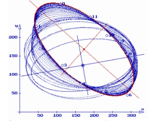
This sum Sgeom depends on five parameters, determining the searched ellipse. The five partial derivatives of Sgeom with respect to the same unknowns B, C, D, E and F equalized with zero determine a nonlinear system of equations, that may be solved with iterative Newton-Raphson method [5], [18], [24], at each step the obtained ellipse fitting better the given points, as we can notice viewing the successive obtained ellipses in figure 2.
Fig. 2. The successive obtained ellipses, the last one ensuring the minimal value of the sum of squared
distances
We assume the reader is familiar with the difficulties of solving simultaneous nonlinear equations.
4. The PROCEDURE of ELLIPSE FITTING BASED on the GEOMETRIC
LOCUS PROPERTIES
There are two possible ellipse definitions based on the geometric loci.
The first asserts that every ellipse point has the constant rate of two distances, first one between the point and a straight line named directrice and the second one between the point and the focus in the proximity of directrice, as shown in figure 3, where are presented an ellipse, the directrice and the two foci. The distance between the ellipse center and the
directrice is 2 2
2
0 ,c a b
c a
CD = = − , knowing the
following property const
a c D E
F E 1 = =
Fig. 3. The first ellipse definition using geometric loci.
As in previous cases, considering m given points in the Oxy plane that have to be fitted by an ellipse, each point have to satisfy the condition:
. const |
C y B x A |
B A ) y y ( ) x x (
k k
2 2 2 1 F k 2 1 F k
= +
+
+ −
+ −
(3)
where A, B and C are coefficients of the directrice equation and xF1 and yF1 are the coordinates of the focus located in the proximity of directrice.
The following expression
) 4 ( C
y B x A
) y y ( ) x x (
C y B x A
) y y ( ) x x ( )
B A ( S
2 2 F 2
F 1 m
1 k
m
k k k
2 F k 2 F k 2
2
+ +
− + − −
−
+ +
− + − +
=
−= =
λ λ
λ λ
λ
has to be minimized, searching adequate values for unknowns A, B, C, xF1 and yF2 .
This task is not possible to accomplish with the required accuracy because the derivatives of this expression and the derivatives necessary to be performed to establish the Jacobian matrix can be computed only using numerical methods, that usually involve large errors, because we must add and subtract many terms with near identical values.
The well known property (the sum of distances between the points on the ellipse and the two foci is constant and equal twice to the semi-major axis) may be used in the procedure of fitting some points with an ellipse.
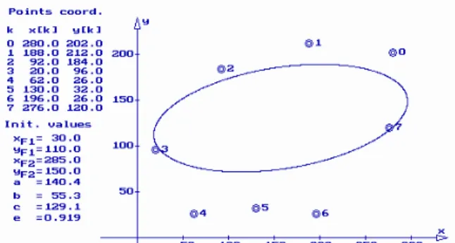
An ellipse that will fit is shown in figure 4. Its five elements that must be determined: the foci coordinates (four unknown) and the semi-major axis (one unknown).
Fig. 4. The second ellipse definition using geometric loci.
If this ellipse definition is considered for a single point in plane, we have the following expression
≠ = −
− − + − +
+ − + − =
error 0
ellipse on
int po 0 a 2
) y y ( ) x x (
) y y ( ) x x ( d
2 2 F 2 2 F
2 1 F 2 1 F
noticing that a deviation is possible when the point does not belong to the ellipse.
The task will consist in the reduction of the sum of squares of these deviations, using an iterative procedure.
2 2 k 2 F 2 k 2 F m 1 k 2 k 1 F 2 k 1 F a 2 ) y y ( ) x x ( ) y y ( ) x x ( S − − + − + − + − + =
=and the values of five parameters
z1=xF1, z2=yF1, z3=xF2, z4=yF2, z5=a
will be determined for obtain the minimal value of S.
Using the notation above, the written the sum becomes 2 5 2 k 4 2 k 3 m 1 k 2 k 2 2 k 1 z 2 ) y z ( ) x z ( ) y z ( ) x z ( S − − + − + − + − + =
= (5)
The method of least squares will be used. The partial derivatives are
0 ) y z ( ) x z ( x z z 2 ) y z ( ) x z ( ) y z ( ) x z ( 2 z S 2 k 2 2 k 1 k 1 5 2 k 4 2 k 3 m 1 k 2 k 2 2 k 1 1 = − + − − − − + − + + − + − = ∂ ∂
= 0 ) y z ( ) x z ( y z z 2 ) y z ( ) x z ( ) y z ( ) x z ( 2 z S 2 k 2 2 k 1 k 2 5 2 k 4 2 k 3 m 1 k 2 k 2 2 k 1 2 = − + − − − − + − + − + − + = ∂ ∂
= 0 ) y z ( ) x z ( x z z 2 ) y z ( ) x z ( ) y z ( ) x z ( 2 z S 2 k 4 2 k 3 k 3 5 2 k 4 2 k 3 m 1 k 2 k 2 2 k 1 3 = − + − − − − + − + − + − + = ∂ ∂
= 0 ) y z ( ) x z ( y z z 2 ) y z ( ) x z ( ) y z ( ) x z ( 2 z S 2 k 4 2 k 3 k 4 5 2 k 4 2 k 3 m 1 k 2 k 2 2 k 1 4 = − + − − − − + − + − + − + = ∂ ∂
= 0 z 2 ) y z ( ) x z ( ) y z ( ) x z ( 4 z S 5 2 k 4 2 k 3 m 1 k 2 k 2 2 k 1 5 = − − + − + − + − + − = ∂ ∂
=and equaling them with zero, the system of five nonlinear equations is obtained
= = = = = 0 ) z , z , z , z , z ( f 0 ) z , z , z , z , z ( f 0 ) z , z , z , z , z ( f 0 ) z , z , z , z , z ( f 0 ) z , z , z , z , z ( f 5 4 3 2 1 5 5 4 3 2 1 4 5 4 3 2 1 3 5 4 3 2 1 2 5 4 3 2 1 1 (6)
and we have to know the initial considered values for the five unknowns. One may write them in symbolic form
t ) 0 ( 5 ) 0 ( 4 ) 0 ( 3 ) 0 ( 2 ) 0 ( 1 ) 0 ( ] z z z z z [ Z , 0 ) Z (
F = = (7)
the vector Z being t
5 4 3 2
1 z z z z ]
z [
Z= .
The system (6) will be solved with Newton’s iterative method, according to the following relations
( )
. . . , 3 , 2 , 1 , 0 i , Z Z Z ) 8 ( , ) Z ( F Z Z J ) i ( ) i ( ) 1 i ( ) i ( ) i ( ) i ( = ∆ + = − = ∆ +where J is the Jacobi’s matrix
) 5 x 5 ( 5 5 1 5 5 1 1 1 z f . . . z f . . . . . . . . . z f . . . z f ) Z ( J ∂ ∂ ∂ ∂ ∂ ∂ ∂ ∂
= (9)
The partial derivatives (the Jacobi’s matrix elements) are numerically computed using the formula [18], [24],
h 12 ) h 2 x ( g ) h x ( g 8 ) h x ( g 8 ) h 2 x ( g x d g
d ≈ − − − + + − +
the expression of one partial derivative, e. g.
j k z
f ∂
∂ being
j 5 j j 1 k 5 j j 1 k 5 j j 1 k 5 j j 1 k j 5 4 3 2 1 k h 12 ) z , . . . , h 2 z , . . . , z ( f ) z , . . . , h z , .. . , z ( f 8 ) z , . . . , h z , . . . , z ( f 8 ) z , . . . , h 2 z , . . . , z ( f z ) z , z , z , z , z ( f + − − + + + − − − − ≈ ≈ ∂ ∂
5. NUMERICAL EXAMPLES
Using the written C program, many results were obtained, which prove the correctness of the method, and also the high precisions of the fitting.
For each case, the initial solution ellipse is presented, followed by a second figure
containing the successive ellipses
corresponding to the performed iterations, the final obtained ellipse, also the values of the objective function which diminishes to a minimal value.
Fig. 5. First example. The given points in the plane and the initial considered ellipse
Fig. 6 First example. The intermediate ellipses and final obtained ellipse. The descending objective function values are as follows: 12437.3 25740.5 7294.4
6118.4 10198.2 2378.7 974.8 675.1 674.5
674.5 …
Observing figures 5 and 7 one may notice that the coordinates of the eight points are the same, the initial considered ellipses are different, and using the presented method one finds the same final results.
Fig. 7. Second example. The given points in the plane and the initial considered ellipse
Fig. 8. Second example. The intermediate ellipses and final resulted ellipse. The successively obtained objective
function values are as follows: 11281.9 1844.1
6064.9 917.4 685.5 674.6 674.5 674.5…
The cases of fitting with twelve and sixteen points and eleven points with an arc of ellipse are shown in the following figures.
As in previous figures, one can see that the obtained ellipses perform a good fitting.
Fig. 10. Third example. The intermediate ellipses and final obtained ellipse. The descending objective function
values are as follows: 36585.9 15862.5 2734.3
12378.4 1412.5 879.6 646.9 634.0 633.3
633.3…
Fig. 11. Fourth example. The given points in the plane and the initial considered ellipse
Fig. 12. Fourth example. The intermediate ellipses and final obtained ellipse. The descending objective function
values are as follows: 18641.7 4018.4 2386.5
1953.2 11208.1 1074.0 563.6 555.7
555.7…
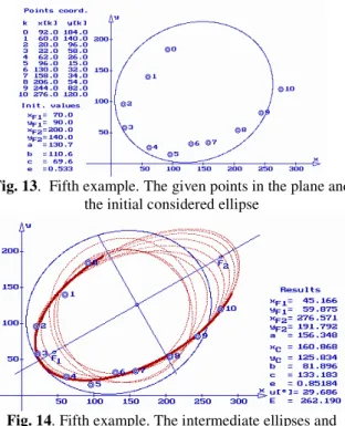
Fig. 13. Fifth example. The given points in the plane and the initial considered ellipse
Fig. 14. Fifth example. The intermediate ellipses and final obtained arc of ellipse. The descending objective function values are as follows: 15062.2 21669.8
15371.8 20200.6 3210.6 626.8 3659.2
292.3 268.1 262.7 262.1
6. CONCLUSIONS and FURTHER WORK
The new discovered method may be considered as a good alternative to the existing methods, the algebraic and geometric fitting with their different variants.
This new method may be seen as a successful combination of the previous cited methods: as in algebraic fitting the expression containing some deviations are minimized, and as in geometric fitting (the so-called best fitting) the iterative procedure is used, so that the objective function is minimized.
The difference is in the construction of the objective function: in the case of algebraic fitting, the deviations are obtained after the introduction of points coordinates in the general equation of conics (of ellipse), while in the case of geometric fitting one minimizes the sum of squared distances between points and ellipse’s contour. In this current method question is to minimize the sum of squared deviations of the ellipse definition, as geometric locus.
Which method is the best one?
examples, varying the number of points, their arrangement in plane, using different numbers of iterations.
The author, disposing the all necessary own created software for mooted methods hopes that will give a documented answer in a future papers.
7. REFERENCES
[1] Ahn, S. J., Rauh, W., Recknagel, M., Geometric fitting of line, plane, circle, sphere and ellipse, ABW-Workshop 3D-Bildverarbeitung an der Technischen Akademie Esslingen, 25-26 I 1999, 8 pp. [2] Ahn, S. J., Rauh, W., Warneke, H.-J.,
Least-squares orthogonal distances fitting of circle, ellipse, hyperbola and parabola, Pattern Recognition, 2001, Vol. 34, No. 12, pp. 2283-2303
[3] Bookstein, F. L., Fitting conic sections to scattered data, Computer Graphics and Image Processing, 1979, vol. 9, pp. 56-71
[4] Chen, S. a. o., A hybrid method for ellipse detection in industrial images, Pattern Recognition, 2017, Vol. 68, pp. 82-98 [5] Engeln-Müllges, G., Uhlig, F., Numerical
Algorithms with C, New York, Springer, 1996, 596 pp.
[6] Fitzgibbon, A., Pilu, M., Fisher, R. B., Direct least square fitting of ellipses, IEEE Transactions on Pattern Analysis and Machine Intelligence, 1999, Vol. 21, No. 5, pp. 476-480
[7] Fornaciari, Michele, Prati, Andrea, Cucchioara, Rita, A fast and effective ellipse detector for embedded vision applications. Pattern Recognition, 2014, Vol. 47, No. 11, pp. 3693-3708
[8] Gander, W., Golub, G. H., Strebel, R., Least-squares fitting of circles and ellipses, BIT 1994, Vol. 34, pp. 558-578 [9] Glavonjić, M., Circles and ellipses fitting to measured data, FME Transactions, 2007, Vol. 35, pp. 165-72
[10] Kanatani, K., Ellipse fitting with hyperaccuracy, IEICE Trans. Inform. Syst., 2006, E89-D, pp. 2653–2660. [11] Kanatani, K., Sugaya, Y., Compact
algorithm for strictly ML ellipse
fitting, Proceedings of 19th International Conference in Pattern Recognition, Tampa, FL., U.S., 2008 [12] Kåsa, I., A circle fitting procedure and its
error analysis, IEEE Transactions on Instrumentation and Measurement, 1976, Vol. 25, pp. 8-14
[13] Libuda, L., Grothues, I., Kraiss, K.-F., Ellipse detection in digital image data using geometric features, in Advances in Computer Graphics and Computer Vision, Springer, 2007, pp. 229-239 [14] Murgulescu, Elena a. o., Analytical and
Differential Geometry, sec. ed. (in Romanian), Editura Didactică şi Pedagogică, Bucureşti, 1965, 772 pp. [15] Ouellet, J.-N., Hébert, P., Precise ellipse
estimation without contour point extraction, Machine Vision and Applications, 2009, Vol. 21(1), pp. 59-67
[16] Pearson, K., On lines and planes of closest fit to systems of points in space, The Philosophical Magazine, 1901, Ser. 6, Vol. 2, No. 11, pp. 559-572 [17] Pratt, V., Direct least-squares fitting of
algebraic surfaces, Computer Graphics, 1987, Vol. 21, pp. 145–152 [18] Press, W. H. a. o., Numerical Recipes in C++. The Art of Scientific Computing, Cambridge University Press, 2003, 1002 pp., ISBN 0-521-75033-4
[19] Rosin, P. I., A note on the least square fitting of ellipses, Pattern Recognition Letters, 1993, Vol. 14, pp. 799-808 [20] Rosin, P. I., Analyzing error of fit functions
for ellipses, British Machine Vision Conference, Pattern Recognition Letters, 1996, Vol. 17, No. 14, pp. 1461-1470
[21] Stricker, M., A new approach for robust ellipse fitting, Int. Conf. Automation, Robotics and Computer Vision, 1994, pp. 940-945
[22] Taubin, G., Estimation of planar curves, surfaces and nonplanar space curves defined by implicit equations, with applications to edge and range image segmentation, IEEE Transactions on
Intelligence, 1991, Vol. 13, No. 11, pp. 1115–1138
[23] Ursu-Fischer, N., Ursu, M., A new and efficient method to perform the circle fitting, Acta Technica
Napocensis, Series: Applied
Mathematics and Mechanics, 2004, No. 47, Vol. III, pp. 21-30, ISSN 1221-5872
[24] Ursu-Fischer, N., Ursu, M.,Numerical Methods in Engineering, (in Romanian), Casa Cărţii de Ştiinţă, Cluj-Napoca, 2019, 836 pp., ISBN 978-606-17-1450-6
[25] Ursu-Fischer, N., Considerations about algebraic fitting of an ellipse to scattered 2D data, Acta Technica
Napocensis, Series: Applied
Mathematics, Mechanics and
Engineering, Vol. 62, Issue II, 2019, ISSN 1221-5872
[26] Ursu-Fischer, N., Popescu, Diana Ioana, Moholea, Iuliana Fabiola, The two stages circle fitting method, Acta Technica Napocensis, Series: Applied
Mathematics, Mechanics and
Engineering, Vol. 62, Issue II, 2019, ISSN 1221-5872
[27] Watson, G. A., Least squares fitting of circles and ellipses to measured data, BIT, 1999, Vol. 39, No. 1, pp. 176-191 [28] Xie, Y., Ji, Q., A new efficient ellipse detection method, Pattern Recognition, 2002, pp. 957-960
O METODĂ ALTERNATIVĂ PENTRU A REALIZA APROXIMAREA CU ELIPSE A UNOR
PUNCTE DIN PLAN
Rezumat: Se poate observa importanţa studiilor privind aproximarea unor puncte din plan cu cercuri sau elipse şi prin faptul că literatura tehnică este foarte bogată în acest domeniu, fiind tratată atât aproximarea algebrică cât şi cea geometrică, cu utilizări în softurile de proiectare. Sunt prezentate pe scurt cele două metode de aproximare, cu precizarea avantajelor şi a dezavantajelor acestora, ambele metode utilizând ecuaţia carteziană a conicelor. Deoarece elipsa se poate defini în două feluri ca un loc geometric, în lucrare se folosesc aceste proprietăţi pentru a realiza aproximarea punctelor cu o elipsă, asigurând precizia rezultatelor, comparativ cu cele două metode cunoscute, elementul comun fiind folosirea aceleiaşi metode a celor mai mici pătrate. Toate aspectele necesare pentru utilizarea metodei sunt prezentate şi multe exemple care justifică avantajele acestei noi metode descoperite.
Nicolae URSU-FISCHER, Prof. dr. eng. math., Dr H. C., Technical University of Cluj-Napoca, Faculty of Machine Building, Department of Mechanical Systems Engineering, 103-105
Muncii Avenue, 400641 Cluj-Napoca, Phone: +40-264-401656, e-mail: