Econ Journal Watch
Scholarly Comments on Academic Economics
Volume 9, Issue 1, January 2012
COMMENTS
WATCHPAD
EJW-MERCATUS SYMPOSIUM
EJW-MERCATUS SYMPOSIUM U.S. SOVEREIGN DEBT CRISIS:
TIPPING-POINT SCENARIOSAND CRASH DYNAMICS
Editor's Notes 1-2
The Unemployment Impact of the 2008 Extension of Unemployment Insurance: As High as Robert Barro Suggested?
Steven D. Mullins 3-20
Introduction to Symposium on U.S. Sovereign Debt Crisis: Tipping-Point Scenarios and Crash Dynamics
Tyler Cowen 21-23
Some Possible Consequences of a U.S. Government Default
Jeffrey Rogers Hummel 24-40
The Bond Market Wins
Garett Jones 41-50
How a Default Might Play Out
Courting an Avoidable Financial Crisis
Joseph J. Minarik 60-70
How and Why a U.S. Sovereign Debt Crisis Could Occur
Editor’s Notes:
Acknowledgments 2010-11
I am grateful to the co-editors Bruce Benson, Fred Foldvary, George Selgin, and Larry White and the managing editor Jason Briggeman for all their fine work, and to readers for their interest and feedback.
We are grateful to Kevin D. Rollins for his friendship and frequent in-a-pinch consultation, to John Stephens for fine-tuning the superb website and document-production system that he created, and to Brett Barkley and Ryan Daza for ongoing occasional service to the journal.
For friendship and vital sponsorship, we are grateful to the American Institute for Economic Research, which officially sponsored the journal from December 2009 through August 2011.
We thank all those who have made donations to our project, and especially the Earhart Foundation, the Charles G. Koch Foundation, Joseph McLaughlin, Gerry Ohrstrom, and Lou Carabini for their faithful support. And we send a special thanks to Walter E. Williams for generous assistance.
We are grateful to the Atlas Economic Research Foundation for their friendship and in-kind support in housing EJW within their organization, especially Romulo Lopez and Brad Lips.
We thank the Mercatus Center at George Mason University for co-organizing and sponsoring the debt crisis symposium appearing in the present issue (January 2012), especially Tyler Cowen, who co-edited the symposium, and Rob Raffety.
We thank the following individuals for helping provide intellectual accountability to EJW:
Referees during 2010-11 Alberto Abadie Harvard University Lloyd Cohen George Mason University Tyler Cowen George Mason University Edward A. Dyl University of Arizona William B. Elliot University of Texas, El Paso
ECON JOURNAL WATCH 9(1)
Peter Gordon University of Southern California Thomas Hazlett George Mason University Robert Higgs The Independent Review
Ben Jacobsen Massey University Garett Jones George Mason University Richard Jong-A-Pin University of Groningen
Arnold Kling Mercatus Center at George Mason University George Leef John William Pope Foundation
Thomas C. Leonard Princeton University Robin Lindsey University of British Columbia Brian Lucey Trinity College, Dublin Bruce McCullough Drexel University Gregory Rehmke Economic Thinking Dani Rodrik Harvard University Alvin E. Roth Harvard University Philip A. Rothman East Carolina University James S. Taylor College of New Jersey Kurt Schuler U.S. Department of Treasury Jane Shaw John William Pope Foundation Alexander Tabarrok George Mason University David L. Weimer University of Wisconsin Robert Whaples Wake Forest University
Replying Authors published 2010-11 Gauti B. Eggertsson Federal Reserve Bank of New York Haifang Huang University of Alberta
Yao Tang Bowdoin College
Other individuals who published comments on EJW material in EJW during 2010-11 C. Fred Bergsten Institute for International Economics Jeffry Frieden Harvard University
The Unemployment Impact of the 2008
Extension of Unemployment Insurance:
As High as Robert Barro Suggested?
Steven D. Mullins
1LINKTO ABSTRACT
My calculations suggest the jobless rate could be as low as 6.8%, instead of 9.5%, if jobless benefits hadn’t been extended to 99 weeks.
—Robert J. Barro,Wall Street Journalop-ed, August 30, 2010
The U.S. unemployment rate averaged 4.6 percent in the two years prior to the economy entering the 2008-09 recession and it more than doubled to 9.5 percent by the summer of 2010 when Robert Barro (2010) estimated how much of that increase was attributable to changes in unemployment insurance (UI) policy. His analysis suggested the recession was not nearly as severe as unemployment statistics suggested because more than half of the increase in the unemployment rate since the recession began was caused by an extension of UI. Barro believes the administration should reconsider extensions of UI benefits.
The unemployment insurance program is a perfect example of government policy that confronts the classic tradeoff between economic efficiency and equality (Okun 1975). The motivation behind the creation of the UI in 1935 was clearly a sense of compassion—to provide temporary help to those suffering income losses during a widespread economic downturn. But this compassion comes at some cost. Inefficiency can result as a consequence of subsidizing the very condition against which UI seeks to protect individuals. Economists have long accepted the theory and evidence that UI benefits are likely to cause extended durations of
Discuss this article at Journaltalk: http://journaltalk.net/articles/5750
ECON JOURNAL WATCH 9(1)
unemployment (Katz and Meyer 1990; Chetty 2008), and some have recommended that the resulting inefficiency is large enough to consider reducing the extent of UI benefits (Barro) or eliminating the current UI program altogether and replacing it with individually pre-funded savings accounts (Feldstein and Altman 1998).
The current recession, with its combination of historically long durations of unemployment (Farber 2011) and unprecedented extensions of UI benefits (U.S. Department of Labor 2011), has generated renewed interest in this policy debate. Proposals to scale back UI benefits are strengthened if recent extensions in the duration of UI benefits are found to have caused large and inefficient increases in the unemployment rate. On the other hand, if these extensions caused only modest increases in unemployment during a deep recession such as 2008-2009, a policy of limiting the extension of benefits may punish those individuals disproportionately suffering from the economic downturn while generating little gain in economic efficiency. Is Barro correct? Has UI caused large, unnecessary increases in unemployment during the Great Recession? What do the most recent data tell us about this important policy question?
Bhashkar Mazumder Estimates the Impact
A number of economists have recently attempted to measure the impact of the Emergency Unemployment Compensation program—created in the summer of 2008—on the national economy’s unemployment rate (U). Most of these studies have first estimated the impact of extended benefits on the average duration of unemployment and then used that estimate to calculate how much such an increase in the duration of unemployment would raise U, ceteris paribus. Bhashkar Mazumder (2011) provided an example of this methodology in a recent article published by the Federal Reserve Bank of Chicago.
Mazumder contrasted the maximum number of weeks of unemployment insurance available during the current recession (99 weeks as of February 2011) with that of the 1982 recession when maximum coverage extended to only 55 weeks. The observed unemployment rate may overstate weakness in the labor market if the unemployed, instead of taking existing job offers, have lengthened the duration of their job search as a consequence of their ability to collect UI benefits for extended periods. Since policymakers rely heavily on unemployment statistics when formulating policy, Mazumder fears that such an increase in the unemployment rate could lead to inappropriate macroeconomic policy decisions (2011, 1).
Mazumder’s method of estimating how much the extension of UI has raised U is based on the steady-state unemployment rate theory that defines the
omy’s equilibrium unemployment rate in terms of the rate of job separation (s, the fraction of the employed who are periodically separated from their jobs) and the rate of job finding (f, the fraction of the unemployed who find employment during the same period). In steady-state equilibrium U must equals/(s+f), and if the recent extension of the maximum duration of UI has lengthened the average duration of unemployment (and thereby reducedf), then extended UI has increased the economy’s steady-state unemployment rate. An estimate of the magnitude of the decline in the job finding rate caused by extended UI can be used to estimate the resulting increase in U, ceteris paribus.
Mazumder obtained an initial value offby assuming that the economy was in a steady state during the six months prior to the July 2008 extension of UI. The unemployment rate averaged 5.1% during that period and the average duration of unemployment was 17 weeks. A seventeen-week average duration of unem-ployment implies a probability of finding a job in any given week of 1/17 or about 0.06, and since the average month has 4.33 weeks, he estimated the initial steady-date monthly rate of job finding to be 0.253. This combined with U = 0.051 implies a job separation rate of 0.0136. These are the base values for f and s he used to estimate how much steady-state U has been increased as a consequence of extended UI (ibid., 2).
The next step in his analysis was to obtain an estimate of how the national average duration of unemployment has been affected by the UI benefit extensions. Mazumder used the finding by Card and Levine (2000) that in a New Jersey extended UI experiment, a one-week increase in the maximum number of weeks of UI benefit eligibility raised the duration of unemployment by 0.1 week. This estimate was applied to the increase in the number of weeks the average eligible unemployed worker could receive UI as of spring 2011, allowing Mazumder to conclude that the average duration of unemployment increased from 17 to almost 20 weeks as a consequence of extended benefits, thus lowering the rate of job finding from 0.253 to 0.22 and raising the steady state unemployment rate by 0.8 percentage points (Mazumder, 2).
As a test of robustness, Mazumder provided alternative estimates by considering other measures of the impact of a week of extended UI eligibility on the duration of unemployment. If an added week of UI benefit eligibility were to increase the duration of unemployment by 0.16 weeks, as estimated by Katz and Meyer (1990), instead of 0.1, then Mazumder’s estimate of the resulting increase in U would be 1.2 points rather than 0.8. He also considered alternative values for the UI take-up rate, or the proportion of the eligible unemployed who do receive benefits. During this recent recession, the take-up rate rose from a pre-recession rate of 0.4 to 0.7. If half of this increase in the take-up rate were assumed to be due to the severity of the current recession and the other half due to the extension
of UI, his estimate of the resulting increase in U would change from 0.8 to 1.1 points. (Mazumder, 3) When he combined the Katz and Meyer larger estimate of the impact of an added week of UI on the duration of U with the higher take-up rate, his estimate of the resulting increase in the unemployment rate was 1.7 points (Mazumder, 4). It is worthy to note that Mazumder’s estimates are much smaller than that obtained by Barro but are consistent with other recent studies Mazumder reviewed that used both similar and alternative methodologies (ibid., 1-2).
Robert Barro Estimates the Impact
A much more damning estimate of the impact of extended UI on the unemployment rate was provided by Robert Barro (2010) in an op-ed entitled, “The Folly of Subsidizing Unemployment” published in the Wall Street Journal. Barro suggested that the June 2010 unemployment rate of 9.5% would have been 2.7 percentage points lower had it not been for the expansion of UI benefit eligibility.
Barro’s methodology is straightforward. He begins, like Mazumder, by noting a stark contrast between unemployment durations in the current recession with those of 1982 when the peak mean duration of unemployment was 21.2 weeks and 24.5% of the unemployed were experiencing joblessness for longer than 26 weeks. In contrast, the duration of unemployment in October of 2009 averaged 27.2 weeks, with 36% of the unemployed out of work for more than 26 weeks. Barro notes that since the end of WWII, the duration of unemployment has averaged less than 21 weeks and the long-term jobless made up less than 25% of the unemployed. Why are the numbers for the current recession so much higher than those in the historical record? “[T]he dramatic expansion of unemployment-insurance eligibility to 99 weeks is almost surely the culprit,” says Barro.
Barro calculates the possible impact of extended unemployment duration on the unemployment rate by first assuming no change in the size of the labor force. He also assumes that the long-term share of the unemployed would have been 24.5% (its July 1983 level) instead of 46.2% (the June 2010 level) had it not been for the expansion of UI. Given these assumptions, 4.2 million persons who would have otherwise been long-term unemployed would instead have taken a job and the unemployment rate would have been 6.8% instead of 9.5%. Barro goes on to conclude that President Obama should blame his economic advisors for not “arguing that a reckless expansion of unemployment-insurance coverage to 99 weeks was unwise economically and politically.”
While Barro admits that his estimate of the impact of extended UI on long-term unemployment and the unemployment rate is “rough,” it is worth noting that
his conclusions are based on two critical assumptions. The first involves the impact of UI on the size of the labor force. In his hypothetical absence of the expansion of UI coverage to 99 weeks “the labor force still equaled the observed value (153.7 million).” Under this assumption, U falls with the elimination of extended UI coverage because 4.2 million long-term jobless persons now take jobs they oth-erwise would have turned down.
Barro does not consider the possibility of an alternative mechanism whereby the elimination of extended UI benefits lowers U because jobless workers who would have otherwise continued their job search (and be counted as unemployed) while collecting extended benefits instead leave the labor force as discouraged workers. In this scenario, reducing UI benefits does lower U officially, but does not in fact increase the absolute number of employed persons.
Barro’s interpretation of the impact of UI is focused exclusively on the first of these two mechanisms, and it is an interpretation that strengthens his position that extending UI benefits was inefficient because it reduces employment by over 4 million persons. If, on the other hand, extended UI raises U because it encourages the jobless to stay in the labor force, then the policy’s economic impact is primarily one of an income transfer to the long-term unemployed that creates no real job losses. Recent analysis of the unemployed in Austria and a review of the existing literature covering other counties (Card et al. 2007) contradict Barro’s interpretation, as, when their unemployment benefits expire, the majority of the unemployed leave the labor force rather than take a job. A recent working paper using data from the Current Population Survey (Rothstein 2011) came to similar conclusions. The impacts of extended UI benefits on unemployment exit, reemployment, labor force exit hazard rates, and on the unemployment rate were estimated. Unemployment insurance extensions were found to have had a larger impact on labor force exit than on reemployment. The December 2010 unem-ployment rate was estimated to be only 0.3 to 0.6 percentage points higher as a consequence (ibid., 3-4).
In addition to his assumption that extended UI benefits reduce employment rather than change job seekers into discouraged workers, Barro also assumed that the severity of the recent recession could not be responsible for extended durations of unemployment.
The administration has argued that the more generous unemployment-insurance program could not have had much impact on the unemployment rate because the recession is so severe that jobs are unavailable for many people. This perspective is odd on its face because, even at the worst of the downturn, the U.S. labor market featured a tremendous amount of turnover in the form of large numbers of persons
hired and separated every month. […] A program that reduced incentives for people to search for and accept jobs could surely matter a lot here. (Barro 2010)
This argument—that the severity of the Great Recession cannot explain the current long average duration of unemployment—brings us to the focus of the present investigation. In a severe recession where UI benefits have been extended by unprecedented lengths, how can we determine how much of the observed increase in the unemployment rate is due to the impact of extended UI as opposed to the downturn’s real impact on job separation and potential job offers?
Recent analysis at the National Bureau of Economic Research used Displaced Workers Survey data to conclude that the 2008-09 recession did experience unusually high job separation rates compared to previous recessions, including that of 1982 (Farber 2011). While the NBER research made no attempt to estimate the impact of the increase in job separation on the unemployment rate, it strongly suggests that any attempt to measure the impact of UI changes must take into account the separate impact of the severity of the recession. The next section of the paper attempts to do just that. Two detrending methods are applied to annual real GDP and annual unemployment rate data in an attempt to quantify the separate influences of the severity of the recession and the extension of UI benefits on changes in the unemployment rate. The first detrending method—a variation of Okun’s Law—explains annual changes in the unemployment rate based on deviations in the growth rate of real GDP. The second method uses the Hodrick and Prescott filter to remove the trend from annual real GDP and unemployment rates to identify their business cycle components. The resulting deviation of real GDP from the HP-filter trend is used to explain cyclical deviations in the unemployment rate. Variables measuring the duration of extended UI benefits are then included in both models to measure the impact of extended UI on the unemployment rate after controlling for the severity of the recession.
Theory and Evidence
Okun’s Law is a rule of thumb describing the historically strong statistical relationship between changes in the unemployment rate and the growth rate of real GDP. Arthur Okun (1962) used quarterly data for the 1947-1960 period to estimate the “first differences”2version of the relationship
2. Okun also defined a “gap” version of the relationship between unemployment and real output by
change in the unemployment rate = a + b*growth rate of real GNP
The focus of Okun’s work was to identify a time series for potential GNP (1962, 2), but what came to be known as Okun’s Law was his statistical documentation of the unemployment-output growth rate relationship (Knotek 2007). That relationship is used in this section to compare observed changes in the unemployment rate during the recent recession with increases that would be predicted based on the historical relationship between GDP growth and unemployment. Regression analysis is used to estimate the impact that the extension of UI has had on the unemployment rate after controlling for the state of the macroeconomy as measured by the annual growth rate of real GDP.
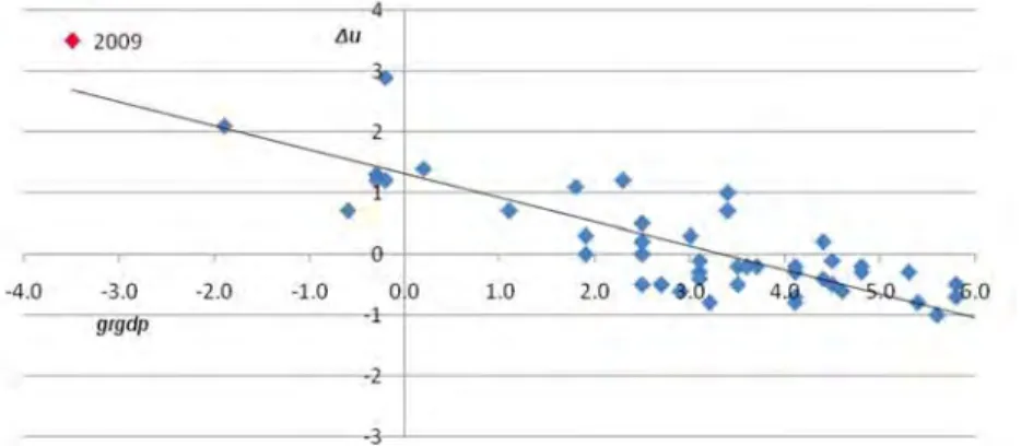
I used annual observations on the growth rate of real GDP (grgdp) (U.S. Bureau of Economic Analysis 2011) and the annual change in the unemployment rate for all civilian workers (Δu) (U.S. Bureau of Labor Statistics 2010) for the 1960-2010 period to obtain an OLS estimate of the “first differences” version of Okun’s Law, Δu= α + β*grgdp. The regression results are shown in equation 1 with the T ratios in parentheses. The R-squared for the estimated equation was .749.
Equation 1: Δu= 1.313 − 0.392*grgdp
(10.4) (−11.98)
The intercept term in Equation 1 provides an estimate of how much the unemployment rate would change in a year of no GDP growth, and the slope coefficient estimates the impact of a one percentage point increase in the GDP growth rate on the annual change in the unemployment rate. Both coefficients are highly significant and are consistent with those obtained by Okun’s original work with quarterly data and more recent work using annual data (Knotek 2007, 80-81).
The estimated regression equation implies that a year of zero GDP growth would cause the unemployment rate to rise a little over 1.3 points and a one percentage point increase in the output growth rate would be associated with an unemployment rate that would be almost 0.4 points lower than otherwise. These estimates are very close to the 1.2 and −0.35 estimates obtained by Knotek (2007) using annual data from the 1949-2006 period, and both sets of estimates suggest that the growth rate of real GDP that is consistent with a steady unemployment rate is about 3.4 percent.3
R-squared measures the proportion of the variation in annual changes in U that can be explained by variation in real GDP growth over the last 50 years. Since almost three-quarters of observed changes in U can be explained by fluctuations in
3. Since Δu= α + β*grgdp, the output growth rate that keeps U constant = −α/β. My estimate of this growth
GDP growth rates, it is clear that this strong cyclical variation in the unemployment rate must be taken into account in any attempt to measure how much of the current relatively high unemployment rate is due to the way job seekers have responded to an extension of UI benefits.
These regression results can be used to control for the impact of the business cycle on unemployment in coming to a rough estimate of the potential impact of extended UI, ceteris paribus. Figure 1 shows the scatter plot of the 50 annual observations4 and the resulting regression line. Any point on the
downward-sloping regression line in Figure 1 shows the annual change in the unemployment rate that one would expect to observe given a growth rate in output.
Figure 1. Δu= f(grgdp) 1961-2010 annual data
The point labeled 2009 in the upper left corner of the scatter diagram shows the unemployment rate change-GDP growth combination for 2009—the worse year of the recession—when real GDP fell by 3.5 percent. Such a decline in GDP would be expected to raise U by 2.7 points above the prior year’s level. However, the actual increase in unemployment from 2008 was 3.5 points. This 0.8 point excess of the observed increase in U over what one would expect given the mag-nitude of the decline in real GDP could be due to the significant increase in the maximum duration of UI from 13 weeks up to 53 weeks that took place in 2009 (U.S. Department of Labor 2011). This rough estimate of the increase in U that could be due to extended UI is at the bottom of the 0.8 to 1.2 point range found by Mazumder and others but it is less than one-third of the 2.7 point increase suggested by Barro (2010).
4. One year’s observation is lost as the unemployment rate variable is the change in U between consecutive
An alternative measure of the severity of the 2008-09 recession and its impact on the unemployment rate was obtained by applying the Hodrick-Prescott filter (Hodrick and Prescott 1997) to the GDP (Backus and Kehoe 1992) and unem-ployment rate data (Mocan 1999) to obtain their HP-filtered trends.5The cyclical
components of GDP and U were then calculated by subtracting the annual observed values from trend. The cyclical component of unemployment (ugap) was regressed on GDP’s deviation from trend (gdpgap) expressed as a percentage of its trend value. The regression results are shown in Equation 2 with the T ratios in parentheses. The R-squared for the estimated equation was .61.
Equation 2:ugap= −0.003 − 0.508*gdpgap
(−.03) (−8.84)
The slope coefficient on gdpgap provides an estimate of how much the unemployment rate deviates from trend for each one percentage point that output deviates from trend. The statistically insignificant intercept term is consistent with the expectation that unemployment will not deviate from its natural level if real GDP does not deviate from trend.
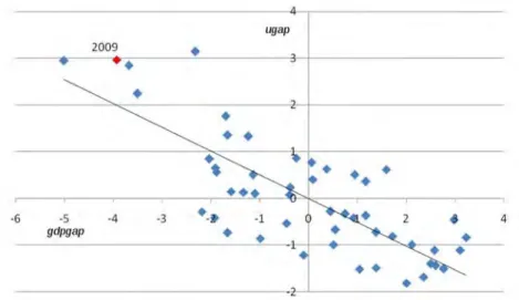
Figure 2 shows the scatter plot for the 1960-2010 annual ugap and gdpgap
observations along with the linear function representing the estimated regression equation. The data point for 2009 is identified, and its deviation from the estimated regression line suggests that the unemployment rate was higher than would be expected given the size of the output gap in than year. Cyclical unemployment is estimated to be 2.0 percentage points when 2009 real GDP is 3.9 points below trend, but the observed gap between the actual unemployment rate and trend was 3 points. This one point excess of the observedugapover what would be expected provides another rough estimate of how much higher unemployment could be a consequence of extended UI. This estimate is also consistent with those found by Mazumder but much less than the 2.7 point increase suggested by Barro.
5. The trends in U and GDP identified by the HP-filter are heavily dependent upon the weight applied to the long-run growth component in the data series. This weight, denoted in the literature as lambda, varies with the frequency of observations. Following Mocan’s work on cyclical unemployment and Bacus’ work on GDP, lambda was set equal to 1600 for the unemployment series and 100 for the GDP series. The debate over appropriate values for this weight is beyond the scope of this paper. See Ravn and Uhlig (2002)
Figure 2.ugap= f(gdpgap) 1960-2010 annual data
A critical limitation of these simple regression models is that there are a number of factors—in addition to the extension of UI—not included in the model specified by Equations 1 and 2 that could have an impact on the unemployment rate. Consequently, the models were estimated again this time adding an additional explanatory variable in an attempt to measure more precisely the impact of the extension of UI benefits on the unemployment rate while controlling for GDP.
Data obtained from the U.S. Department of Labor documenting the effective date of special UI benefit extensions and the length of those extensions was used to construct a variable (xui) measuring the number of additional weeks of unemployment benefits that were available to covered workers during each year over the 1960-2010 period (U.S. Department Of Labor 2011). During some years, extended UI benefits were not available over the entire year, in which case the number of extended weeks of benefits was calculated by multiplying the maximum number of weeks that benefits were payable by the fraction of the year they were available.6
The simple inclusion of the annual change inxui (Δxui) in Equation 1 or
xui in Equation 2 as additional explanatory variables is likely to produce biased
6. Thexuivariable measures the number of weeks of extended unemployment benefits that were available over the year. In years when no extended benefits were availablexuiwas set to 0. During the two years following the 9-11 attacks, for example, UI was extended by 26 weeks beginning in March of 2002 and those extensions were continued until the end of 2003 at which point in time they were phased out. The 2002 value ofxuiwas set equal to 10/12*26 = 21.67 since 26 weeks of benefits were only available for 10 months of that year. The 2003 value forxuiwas set equal to 26 because 26 weeks of extended benefits were
estimates of the impact of changing durations of UI benefits on the unemployment rate because annual changes in xui are sure to have both exogenous and endogenous components. OLS regression is expected to provide unbiased estimates of the impact of extended UI on the unemployment rate under the assumption thatxuiis exogenous and the direction of causation runs only from changes in weeks of extended UI benefits to changes in the unemployment rate. A correct specification of the model must take into account the endogenous behavior of the duration of unemployment benefits because legislation extending UI benefits is clearly influenced by the state of the economy and the actual unemployment rate, although with a consistent lag (Coven and Stone 2008).
Two versions of each of the models defined by Equations 1 and 2 are specified with the addition of an extended UI independent variable in ways that avoid this likely bias. The first version of this specification—Okun1 and HP1—include Δxuiandxuias additional independent variables respectively, but also include the lagged value of the dependent unemployment variable as a third independent variable in order to control for the impact of previous labor market conditions that could inflate the estimate of the impact of UI on U. The resulting specifications of the two models, which include both a UI and a lagged dependent variable on the right hand side, are:
Okun1: Δu= α + β*grgdp+ γ*Δxui+ δ*lagΔu
HP1:ugap= α + β*gdpgap+ γ*xui+ δ*lag ugap
A second version of the two models adds a UI variable that is constructed to remove the endogenous component of variations in UI policy so that the new variable captures only exogenous variation in the extent of UI benefits. This variable was obtained by regressingxui(weeks of extended UI eligibility) on lagged values of the GDP gap and U gap variables and saving the residuals as a new variable,xuishock. This new variable should better capture variation in the extent of UI benefits that are due to changes in the national political landscape over time.7
This new variable is a ‘generated regressor,’ and Pagan (1984) demonstrated that OLS regression models containing explanatory variables derived from predicted and residual values from prior regressions suffer from a version of the errors-in-variables problem. Consequently, the standard errors and resulting t ratios should be used with caution.8
The addition of xuishock and Δxuishock—the annual change in
xuishock—results in the following specifications of the two models.
7. As a test of this expectation,xuishockwas regressed on three dummy variables representing Democratic Party control of the Presidency, the House and the Senate. Democratic control over the Senate was found
Okun2: Δu= α + β*grgdp+ γ*Δxuishock
HP2:ugap= α + β*gdpgap+ γ*xuishock
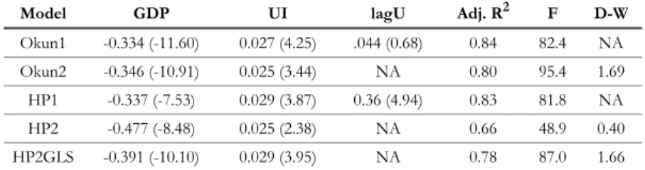
Of particular interest for this research is the sign and significance of γ, the slope coefficient on the variables measuring the weeks of extended UI eligibility. In the two Okun versions of the model, the γ coefficient denotes how much the unemployment rate would change in a given year for every one additional week that UI benefits are extended, ceteris paribus. The γ term in the two HP versions express a similar relationship, only in terms of unemployment’s deviation from trend for every week of extended UI. Each of the models was estimated with OLS regression and the results are presented in Table 1 below.
TABLE 1. Summary Regression Results (t stats) Okun Model Dependent Variable = Change in Unemployment Rate
HP Model Dependent Variable = Unemployment Rate Deviation from HP Trend Model GDP UI lagU Adj. R2 F D-W Okun1 -0.334 (-11.60) 0.027 (4.25) .044 (0.68) 0.84 82.4 NA Okun2 -0.346 (-10.91) 0.025 (3.44) NA 0.80 95.4 1.69 HP1 -0.337 (-7.53) 0.029 (3.87) 0.36 (4.94) 0.83 81.8 NA HP2 -0.477 (-8.48) 0.025 (2.38) NA 0.66 48.9 0.40 HP2GLS -0.391 (-10.10) 0.029 (3.95) NA 0.78 87.0 1.66
The estimated impact of extended UI benefit durations is very consistent in all four models, and slope coefficient estimates on the GDP and UI variables are all of the expected signs and are statistically significant at the alpha=.011 level or better. The estimates of γ obtained from the Okun specification of the model suggest that each one week extension of UI benefits raises the unemployment rate by 0.025 to .027 points, ceteris paribus. The HP specifications are quite consistent as well, with each additional week of extended UI estimated to raise unemployment’s deviation from trend by .025 to .029 points.
Since time series regression analysis is typically prone to serial correlation resulting in untrustworthy standard errors and t-ratios, the residuals were examined and the Durbin-Watson test statistic for autocorrelation was calculated for the Okun2 and HP2 models. The Durbin-Watson dis not reported for the Okun1 and HP1 models because it is not a valid test for autocorrelation when the model contains the lagged dependent variable as a regressor (Durbin 1970), so an
8. There are additional technical issues associated with the use of generated regressors that go beyond the scope of this paper. My thanks go to a referee for bringing them to my attention. Interested readers should
alternative test was used for those models.9 The Okun versions of the model
demonstrated no evidence of serial correlation—most likely due to the first-differencing of the data in those models—but this was not the case for the models using the HP filtered data. Durbin’s alternative test confirmed the presence of autocorrelation in the HP1 model and examination of the residuals from the HP2 regression combined with a d statistic much lower than the critical value for dl
confirmed the presence of first-order autocorrelation in that model as well (Gujarati 2006; Studenmund 2006). In order to correct for serial correlation, HP2 was re-estimated using generalized least squares with the following specification.
HP2GLS:
ugapt− ρ*ugapt−1= α + β*(gdpgapt− ρ*gdpgapt−1) + γ*(xuishockt− ρ*xuishockt−1)
Rho (ρ) was estimated to be .80 and the resulting GLS regression results are provided in the last row of Table 1.10The residuals from this regression showed
no sign of first-order autocorrelation, anddincreased to 1.66, which exceedsdu,
the upper bound of the indeterminate range ford. The resulting estimates of the impact of the GDP gap and extended weeks of UI on the unemployment rate are still significant and of the expected signs.
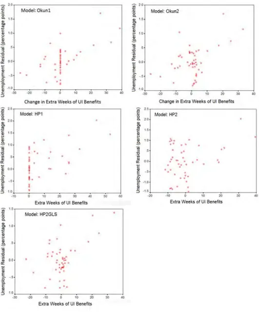
A visual indication of the relationship between extended UI benefits and unemployment is provided by the partial residual plots in Figure 3 (Larsen and McCleary 1972). Each of the five plots—one for every model specification—is formed asres+ γ*uiwhereresare the regression residuals from the model and γ is the regression coefficient onui, the relevant variable from each model.
These regressions attempt to measure the impact of extended UI on the unemployment rate holding GDP constant. If it were the case that extended benefits reduced GDP while they raised unemployment, my estimate of the impact of UI on unemployment would be biased downward. But a body of research suggests that this scenario is unlikely, as the majority of the unemployed whose UI benefits are exhausted leave the labor force instead of going back to work (Card et al. 2007; Rothstein 2011). Those individuals whose employment is not influenced by extra UI are certainly picked up in my regressions.
9. The residuals from the Okun1 and HP1 OLS regressions were regressed on all regressors in each model plus the lag of the residuals. The t ratio for the coefficient on the lagged residual was then used to test for the presence of serial correlation.
10. An estimate of ρ was obtained by regressing the residuals from the HP2 regression on their lagged
Figure 3. Partial residual plots for the UI variable
How Do These Results Compare to Barro’s
Estimate of the Impact of Extended UI?
The regression results described in the previous section were used to
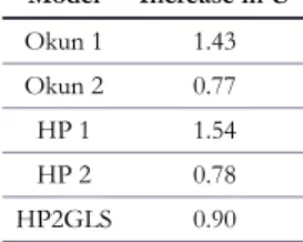
of the extension of UI benefits, ceteris paribus. Table 2 shows the results of these calculations. The regression coefficient on the UI variable in each of the five specifications of the model was multiplied by the relevant independent UI variable to estimate how much the unemployment rate was increased as a consequence of the increases in the duration of UI benefits that occurred since the Emergency Unemployment Compensation program was created in the summer of 2008. The estimates derived from the two Okun models are percentage point increases in the unemployment rate in 2010, while the HP model estimates are the percentage point increases in the excess of the observed unemployment rate over the trend unemployment rate. These estimates are larger than those provided by Rothstein (2011) but are very close to the 0.8-1.7 point range obtained by Mazumder (2011, 2). They are, however, lower than the 2.7 point estimate provided by Barro (2010).
TABLE 2. Estimated Impact on 2010 Unemployment Rate of
Extended UI Model Increase in U Okun 1 1.43 Okun 2 0.77 HP 1 1.54 HP 2 0.78 HP2GLS 0.90
Summary and Conclusions
The models developed in the previous section estimate that the unemployment rate would have been between 0.77 and 1.54 points lower in 2010 had it not been for the unprecedented increases in the duration of UI benefits that occurred since the Emergency Unemployment Compensation program was created in the summer of 2008. These results are contrasted with those provided by Barro (2010), who assumed that all of the observed increase in long-term unemployment during this recession was due to extended UI, and that if it were not for those extensions the unemployment rate would have been 6.8 percent in the summer of 2010 instead of 9.5. Another estimate (Mazumder 2011) based on steady-state unemployment theory found that the unemployment rate would have been in the 7.8 to 8.7 percent range in the absence of extended UI benefit durations. The present paper controls for the severity of the recession and finds that the 2010
unemployment rate would have been between 8.0 and 8.8 percent if it were not for extended UI benefits.
While my research indicates that Barro’s assessment of the impact of UI on unemployment may be exaggerated, one important point to glean from all of these estimates is that policymakers have good reasons to use caution when considering the unemployment rate as a guide to macroeconomic policy, especially during periods when an extension of UI benefits has pushed the unemployment rate above levels that would have prevailed otherwise.
Appendices: Data and Regression Output Files
GDP and U detrended with HP FilterThis Excel file contains real GDP and the unemployment rate for the 1960-2010 period. Deviations in real GDP from trend (as a % of trend GDP) and deviations in U from its trend are calculated using the Hodrick-Prescott Filter.
SPSS file with dependent and independent variables for all regressionsThis file contains all of the dependent and independent variables used in the Okun and HP models as well as the transformed data for the GLS estimate of the HP2 model. The residuals from all models are also saved here and used to create the partial residual plots.
These files contain the SPSS output for each of the five regression models.
SPSS Output for Okun 1 Model SPSS Output for Okun 2 Model SPSS Output for HP 1 Model SPSS Output for HP 2 Model SPSS Output for HP 2 GLS Model
References
Backus, David K. and Patrick J. Kehoe. 1992. International Evidence on the Historical Properties of Business Cycles. American Economic Review 82: 864-888.
Barro, Robert. 2010. The Folly of Subsidizing Unemployment.Wall Street Journal, August 30.Link
Card, David, Rah Chetty, and Andrea Weber. 2007. The Spike at Benefit Exhaustion: Leaving the Unemloyment System or Starting a New Job?
American Economic Review97(2): 113-118.
Card, David, and Phillip B. Levine. 2000. Extended Benefits and the Duration of UI Spells: Evidence from the New Jersey Extended Benefit Program.
Journal of Public Economics78: 107-138.
Chetty, Rah. 2008. Moral Hazard versus Liquidity and Optimal Unemployment Insurance.Journal of Political Economy116(2): 173-234.
Coven, Martha and Chad Stone. 2008. The Unemployment Rate Is Already High Enough to Warrant Extended Benefits.CBPP Working Paper. Center on Budget and Policy Priorities (Washington, D.C.).
Durbin, James. 1970. Testing for Serial Correlation in Least Squares Regressions When Some of the Regressors Are Lagged Dependent Variables.
Econometrica38(3): 410-421.
Farber, Henry S. 2011. Job Loss in the Great Recession: Historical Perspective from the Displaced Workers Survey, 1984-2010. NBER Working Paper
17040. National Bureau of Economic Research (Cambridge, Mass,).
Feldstein, Martin and Daniel Altman. 1998. Unemployment Insurance Savings Accounts. NBER Working Paper 6860. National Bureau of Economic Research (Cambridge, Mass,).
Gujarati, Damodar N. 2006.Essentials of Econometrics. New York: McGraw-Hill/ Irwin.
Hodrick, Robert and Edward C. Prescott. 1997. Postwar U.S. Business Cycles: An Empirical Investigation.Journal of Money, Credit and Banking29(1): 1-16.
Katz, Lawrence F. and Bruce D. Meyer. 1990. The Impact of the Potential Duration of Unemployment Benefits on the Duration of Unemployment.
Journal of Public Economics41(1): 45-72.
Knotek, Edward S. II. 2007. How Useful Is Okun’s Law?Federal Reserve Bank of Kansas City Economic Review(Fourth Quarter): 73-103.
Larsen, Wayne A. and Susan J. McCleary. 1972. The Use of Partial Residual Plots in Regression Analysis.Technometrics14(3): 781-790.
Mazumder, Bhashkar. 2011. How Did Unemployment Insurance Extensions Affect the Unemployment Rate in 2008-10?Chicago Fed Letter(285): 1-4.
Mocan, H. Naci. 1999. Structural Unemployment, Cyclical Unemployment, and Income Inequality.Review of Economics and Statistics81(1): 122-134.
Okun, Arthur M. 1975.Equality and Efficiency, The Big Tradeoff. Washington D.C.: Brookings Institute.
Steven Mullinsreceived his Ph.D. in economics from
Oklahoma State University in 1983. He is currently Professor of Economics in the Breech School of Business Administration at Drury University in Springfield, Missouri, where he teaches a variety of economics courses including macroeconomics and econometrics. His research interests include macroeconomic influences on U.S. poverty and the impact of tax reform on the distribution of after-tax income. His firm, Mullins
Econometrics, provides consulting services in a wide variety of legal cases such as workplace injury, wrongful termination, and patent disputes. As an aviation
enthusiast he builds and flies experimental aircraft in his spare time. You can contact him at [email protected].
Statistics Section of the American Statistical Association. Cowles Foundation, Yale University (New Haven, Conn.).
Oxely, Les and Michael McAleer. 1993. Econometric Issues in Macroeconomic Models with Generated Regressors.Journal of Economic Surveys7(1): 1-40.
Pagan, Adrian R. 1984. Econometric Issues in the Analysis of Regressions with Generated Regressors.International Economic Review25(1): 221-247.
Ravn, Morten O. and Harald Uhlig. 2002. On Adjusting the Hodrick-Prescott Filter for the Frequency of Observations. Review of Economics and Statistics
84(2): 371-376.
Rothstein, Jesse. 2011. Unemployment Insurance and Job Search in the Great Recession. Working paper.Link
Studenmund, A. H. 2006.Using Econometrics. Boston: Pearson/Addison Wesley.
U.S. Bureau of Economic Analysis. 2011.National Economic Accounts.Link
U.S. Bureau of Labor Statistics. 2011. Labor Force Statistics from the Current Population Survey.Link
U.S. Department of Labor. 2011.All Special Extended Benefits Programs.Link
About the Author
Go to Archive of Comments section Go to January 2012 issue
Discuss this article at Journaltalk: http://journaltalk.net/articles/5750
EJW-MERCATUS SYMPOSIUM U.S. SOVEREIGN DEBT CRISIS:
TIPPING-POINT SCENARIOSAND CRASH DYNAMICS
Introduction to Symposium on
U.S. Sovereign Debt Crisis:
Tipping-Point Scenarios
and Crash Dynamics
Tyler Cowen
1LINKTO ABSTRACT
We now live in an age of financial crises. My reading is that, unbeknownst at the time, the 1990s were a kind of warm-up act, featuring the Mexico financial crisis, the Asian financial crisis, and the troubles at Long-Term Capital Management. The years 2007-2009 brought a full-scale financial crisis to the United States, only a year or two after talk of “The Great Moderation” had become the conventional macroeconomic wisdom. Suddenly the United States was on the verge of a financial meltdown.
In 2011 the major crisis was in the Eurozone, where Greece, Italy, Spain, Portugal, and Ireland deal with the risk of default. The survival of the Eurozone is now seriously doubted. It is also commonly believed that the troubles of the periphery nations might lead to contagion effects that would severely damage France, Belgium, Finland, and other nations. Our times are now truly scary.
2011 was also notable for the near-default of the United States, based on a budget gridlock in a dysfunctional Congress, and for America’s loss of its traditional AAA credit rating. We are no longer as invulnerable as we once seemed. When it comes to a sovereign debt crisis, it is no longer possible to say “it can’t happen here.” Right now we are borrowing about forty cents of every Discuss this article at Journaltalk:
http://journaltalk.net/articles/5751
dollar the federal government spends, and the imbalance has no end in sight. The American electorate has dug in against both major tax increases and major spending cuts. Super-low borrowing rates have made it all the more tempting to maintain and indeed extend budget deficits. Keynesian economics promises that more government spending will stimulate the economy and create jobs.
More and more economists and budget commentators believe we are in for a rude awakening, and I don’t mean thirty or forty years down the road. I mean within the next ten to twenty years or maybe sooner. Yes, U.S. bond rates are remarkably low, but they were low for a lot of the Eurozone just a few years ago. It is possible that the low rates reflect the precariousness of the situation, and the lack of alternative outlets for invested funds, rather than any rosy picture of America’s fiscal future. Today, an attitude of fiscal complacency would be very risky, especially since the United States government has not settled on any credible plan to stop running budget deficits, even in the longer term.
And that is why EJW and the Mercatus Center at George Mason University have undertaken this symposium: To produce and disseminate a better under-standing of what a sovereign debt crisis in the United States would look like and what might bring it about.
The sorry truth is that recent crises were developments for which the world was quite unprepared. To a large extent we have suffered from a failure of imagination. Academics have been remiss in formulating and thinking through a suitable range of possibilities.
So we bring you these essays, in the hope that it’s not too late for them to make a difference. The authors were invited to speculate on possible tipping points and associated triggers, and on crash dynamics—what happens in the crisis. The authors were encouraged to imagine possible futures, not merely as financial analysts but as political economists. We are grateful to the contributors, Jeffrey Rogers Hummel, Garett Jones, Arnold Kling, Joseph Minarik, and Peter Wallison, for their fine work. We believe the essays can help everyone going forward.
Tyler Cowenis the Holbert C. Harris Professor of Economics at George Mason University and General Director of the Mercatus Center. His latest book isThe Great Stagnation: How America Ate All the Low-Hanging Fruit of Modern History, Got Sick, and Will (Eventually) Feel Better.
About the Author
Go to archive of Watchpad section Go to January 2012 issue Go to Mercatus Center symposium presentation page
Discuss this article at Journaltalk:
http://journaltalk.net/articles/5751
EJW-MERCATUS SYMPOSIUM U.S. SOVEREIGN DEBT CRISIS:
TIPPING-POINT SCENARIOSAND CRASH DYNAMICS
Some Possible Consequences of a
U.S. Government Default
Jeffrey Rogers Hummel
1LINKTO ABSTRACT
Few now doubt that the U.S. government is rushing headlong toward a major fiscal crisis. Promised future outlays, mainly for Social Security, Medicare, and Medicaid, far exceed projected future revenue. The size of the fiscal gap is very sensitive to both demographic changes and economic fluctuations.
The latest estimate of Laurence J. Kotlikoff (2011) puts the gap’s present value at the bone-crushing level of $211 trillion. A more modest estimate from Jagadeesh Gokhale and Kent A. Smetters (2006, 203) estimates the gap as of 2010 at $79.4 trillion. The Congressional Budget Office’s (CBO’s) most recent long-term outlook (2011, 80) has federal expenditures in its Alternative Fiscal Scenario—not counting interest on the accumulating national debt—rising by 2085 to nearly 35 percent of GDP whereas revenues will still be below 20 percent of GDP, a shortfall of almost 15 percent. Marc Joffe (2011), a former employee of Moody’s Analytics, projects that by 2040 the national debt will have already reached more than 180 percent of GDP and that interest alone will swallow nearly 40 percent of federal revenue.
These projections admittedly assume no drastic entitlement or tax changes in the future. I have argued elsewhere (Hummel 2007, 2009, 2010; Henderson and Hummel forthcoming) that (a) federal tax revenue will never consistently rise much Discuss this article at Journaltalk:
http://journaltalk.net/articles/5752
ECON JOURNAL WATCH 9(1) January 2012: 24-40
above 20 percent of GDP (and certainly not above the 25 percent that federal taxes never quite reached during World War II), (b) politicians have little incentive to come up with the requisite expenditure cuts in time, and (c) monetary expansion and its accompanying inflation will no more be able to close the fiscal gap than would an excise tax on chewing gum. Here I explore the consequences, given those three likely constraints, of the only possible alternative: a very substantial default by the U.S. government on Treasury securities. Once a tipping point is reached, such a default will probably unwind swiftly, leaving American politicians with no other options. Whether the default will result in a restructuring that only reduces the U.S. government’s debt burden or in something approaching a more complete repudiation is impossible to foretell. Either way, the short-run consequences for the economy will be painful. But the long-run consequences, both economic and political, could be beneficial, and the more complete the repudiation, the greater the benefits.
The Cascade into Default
The financial structure of the U.S. government has two nominal firewalls. The first, between Treasury debt and unfunded liabilities, is provided by the trust funds of Social Security, Medicare, and other, smaller federal insurance programs. These permit the illusion that the shaky fiscal status of social insurance has no direct effect on the government’s formal debt. But according to the latest intermediateprojections of the Trustees, the Hospital Insurance (HI-Medicare Part A) trust fund will be out of money in 2024, and the Social Security (OASDI) trust funds will run out in 2036. Thepessimisticprojections have Hospital Insurance empty by 2017 and Social Security by 2030.2
Whenever the trust funds are exhausted, payroll taxes will be insufficient and general revenues will have to finance these programs. Although other parts of Medicare and all of Medicaid already dip into general revenues, when HI and OASDI need to do so, the first firewall will vanish. Anticipation of this event is a potential tipping point, stripping away any illusion that the Treasury’s ability to service its more formal debt is somehow independent of the unfunded liabilities of Social Security and Medicare. If investors react by requiring a risk premium on Treasury securities, the cost of rolling over the national debt will immediately rise. As of September 2011, 15 percent of the Treasuries held by the general public
2. Boards of Trustees of the Federal Hospital Insurance and Federal Supplementary Medical Insurance Trust Funds (2011, 38, 71) and Board of Trustees of the Federal Old-Age and Survivors Insurance and
(including the Fed), or nearly $1.5 trillion, were Treasury bills, which mature in less than one year (Bureau of the Public Debt 2011). A self-reinforcing cycle, in which the rising risk premium exacerbates the federal government’s financial straits, would further raise the premium. Events would then move very fast, much like the collapse of the Soviet Union in 1990-1991.
The second financial firewall is between U.S. currency and government debt. The Federal Reservecouldunleash the Zimbabwe option. My expectation is that, faced with the alternatives of seeing both the dollar and the debt become nearly worthless or defaulting on the debt while saving the dollar, the U.S. government will choose the latter. Russia in 1998 is just one recent example of a government choosing partial debt repudiation over a collapse of its fiat currency (Chiodo and Owyang 2002).
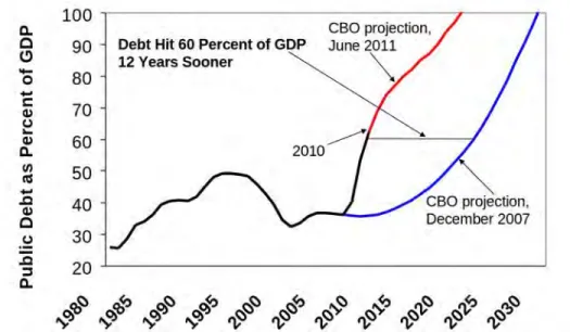
Other events of course might serve as tipping points. In their extensive studies of past financial crises, Carmen M. Reinhart and Kenneth S. Rogoff (2009, 2010) have suggested that a government debt equal to 100 percent of GDP has passed a dangerous threshold. Both the CBO, in its Alternative Fiscal Scenario, and Marc Joffe project that the U.S. will breach this threshold soon after 2020. Paul Krugman (2010a, 2010b) disputes the significance of the 100-percent threshold. The U.S. national debt reached over 100 percent of GDP during the Second World War, and the United Kingdom was able to successfully manage and reduce a World War II-government debt that had climbed all the way to 250 percent of GDP.
Perhaps a more meaningful indicator is interest on government debt as percent of total revenue. This ratio varies not only with the debt’s size but with changes in government revenue and interest rates. Doug Elmendorf (2009, slide 11), director of the CBO, provides some sobering calculations. The report’s Alternative Fiscal Scenario estimated that if federal revenues remained in the neighborhood of 20 percent of GDP for the next 75 years, while federal expenditures net of interest rose to 35 percent of GDP (roughly similar to the 2011 CBO estimate), adding interest payments from the accumulating national debt would drive total federal expenditures up to 75 percent of GDP by 2083, and that would entail interest amounting to a fantastic 40 percent of GDP. Obviously government finances will have reached an explosive tipping point long before that level is ever reached.
Short-Run Consequences of Default
mainly the Social Security and Medicare trust funds. So the conventionally cited figure is the $10,127,031 million held by the public (including the Federal Reserve System), 67 percent of GDP (see Table 1 for comparable numbers as of second quarter of 2011). Even economists debate which is the more relevant number. Yet if one is concerned about the looming fiscal gap, then one needs to add not just the trust funds but the remainder of the fiscal shortfall, yielding as mentioned above a total variously estimated between $79 trillion and $211 trillion. For analyzing the short and long-run consequences of a Treasury default, how to count the trust funds diminishes in importance. By the time a fiscal crisis occurs, the trust funds will already have been depleted, whereas the amount held by the public will have increased. We can therefore concentrate on who among the “public” holds the debt, under the probable assumption that the relative proportions will not alter too much as the debt grows (see Tables 2 and 3).
The Federal Reserve, which is anomalously considered part of the public in official reports, holds about $1.6 trillion in Treasury securities as of September 2011, or almost 17 percent of the publicly held debt (Financial Management Service 2011). That percentage is not much higher than it was before the enormous increase in the Fed’s balance sheet brought on by the recent financial crisis. It could grow substantially if the Fed monetizes more Treasury debt, unless the Fed sterilizes its purchases by selling off its nearly $1 trillion worth of mortgage-backed securities and assorted miscellaneous assets. But to the extent that the Fed is now paying interest on bank reserves (and at a rate that exceeds the return on short-term Treasuries), this portion partly represents indirect holdings of private commercial banks and other depositories.
About 45 percent of the publicly held U.S. Treasuries is owned abroad, more than three-quarters of that by foreign governments and their central banks (Bertaut and Tryon 2007; Hamilton and Wu forthcoming; Reitz 2011). China is the largest foreign investor in U.S. Treasuries, with its holdings (both government and any nominally private) combining to $1.137 trillion as of August 2011, or about a quarter of foreign holdings (Department of the Treasury/Federal Reserve Board 2011).
expenses (including any interest on reserves), as well as finance other government expenditures. More disturbing is the prospect that the Fed might then put new money into circulation by purchasing other private securities, making it an even bigger player in private financial activities and the allocation of savings than it has already become as a result of the financial crisis.
If a total repudiation took place today, initial direct losses to the U.S. private sector would total about $4 trillion, significantly less than any estimate of the U.S. government’s enormous fiscal gap, even less than the $10 trillion fall in the value of the U.S. stock market between 2007 and 2008, and about equal to the fall in the value of U.S. real estate between 2007 and 2009 (Federal Reserve Board of Governors 2011, 94, 106). Outside of the household sector, with its unknown amount of hedge and trust fund holdings, the largest total dollar losses would fall on mutual funds, state and local governments and their retirement funds, and private pension plans. Looking at the overall portfolios within these sectors, the heaviest hit would be money market funds, whose holdings of Treasuries constitute 13 percent of their total assets. Other mutual and closed-end funds hold only a little more than 3 percent of their portfolios in Treasuries. But for private pension funds, the proportion is 8 percent, and for state and local government retirement funds, 6 percent. Commercial banks are still the economy’s most important financial intermediaries, holding $10 trillion in total assets. Treasury securities are only 1.7 percent of that total (although government agency and GSE-guaranteed securities constitute a whopping 13.0 percent).
Admittedly such a crude reckoning ignores an array of secondary effects. Treasuries serve as collateral for other loans in a complex and interconnected financial structure in which savings often passes through two, three, or more layers of intermediation. Default will reverberate throughout credit markets, imposing losses on financial institutions with little direct exposure to government debt. The short-run economic consequences could be very severe and possibly trigger unfortunate political interventions. It is easy to conjure up apocalyptic scenarios of the sort that stampeded Congress into adopting the infamous TARP and that are now terrifying European governments. But the realism of such scenarios is open to question.
offsetting liability that will likewise decline. And that brings us to the potentially desirable long-run consequences.
Long-Run Consequences of Default
The most important long-runpoliticalbenefit of a Treasury default would be that it would make it more difficult for the U.S. government to borrow money. In other words, a default is a balanced-budget amendment with teeth, as David D. Friedman once put it. Sadly, that characterization is not strictly correct. Many defaulting governments have proved able to go back into the loan markets soon thereafter, although often at higher interest rates. Still, a default would help to encourage both greater fiscal responsibility and lower total expenditures on the part of the U.S. government.
A Treasury default would also bring long-run economic benefits. Loan transactions have two parties, the lender (or creditor) who forgoes the current use of money in exchange for a financial asset, and the borrower (or debtor) who gains the current use of money in exchange for a financial liability. All debt, whether private or public, therefore has both an asset side and a liability side. A sudden and unanticipated repudiation of a private debt, so long as no one expects it to be repeated or extended to other debts in the future, has only a distribution effect: The debtor gains by the exact same amount that the creditor loses, with no net wealth effect.
So where is the offsetting liability created by government debt? Although superficially it appears that government itself bears the liability, this impression misses the underlying economic reality. The liability ultimately rests on taxpayers, because their taxes will be almost the entire source of revenue to pay interest and, less frequently, the principal on the government debt. For nearly every financial asset created by government borrowing, therefore, a corresponding tax liability exists. Even if the debt is perpetually funded and never repaid, the discounted present value of this stream of future taxes roughly equals the total value of the debt.
the total value of both privately issued assets, such as shares of stock and corporate bonds, and expected future wage income.
If Ricardian Equivalence does not hold, and people do not perfectly anticipate their future tax liabilities, then they erroneously believe that Treasury securities represent net wealth. Suffering from what is sometimes called “bond illusion” or “fiscal illusion,” they think they are wealthier than they actually are. Whether this illusion has desirable or undesirable economic consequences is one of the many questions involved in economic controversies over business cycles, fiscal policy, and economic growth. Regardless of the answers to these questions, repudiation of the national debt will bring people’s perception of their net wealth into better alignment with reality. They will still enjoy a reduction in future taxes despite never having realized that they would have had to pay them.
Repudiation of Treasury securities held abroad will entail a long-run net gain for Americans. Constituting a transfer to a wealthy U.S. from the rest of the world, this distribution effect may appear unfair. But it has the advantage of ending the coerced support paid to foreign governments, particularly China, by U.S. taxpayers. Indeed, we should keep in mind that the frequent and much-touted bailouts of governments to help them avoid or palliate sovereign defaults, such as of Mexico in 1994, usually end up benefiting creditors, who have willingly taken on the risk of loaning money to governments, at the expense of taxpayers in the “bailed out” country. Such will probably be the consequence of the ongoing fiscal crisis in Greece; and it repeats a pattern that dates back at least as far as the notorious U.S. military interventions into Latin America early in the twentieth century (Langley 1989).
Repudiation of the domestically held national debt would bring no change in net wealth, should Americans perfectly anticipate their future tax liabilities. Moreover, the existence of offsetting tax liabilities serves to mitigate the domestic distribution effects of repudiation. Since nearly everyone pays taxes or owns assets whose value is reduced by taxation, even many who hold government debt will gain overall. They will find over the long run that, as their government securities are wiped out, their other assets rise in value. Even if people do not perfectly anticipate future tax liabilities, they clearly anticipate a part of them, so there should be some compensating rise in the value of private assets.
that a non-trivial number of the government’s creditors will be helped more than they are harmed in the long run.
Those anticipating benefits from Social Security, Medicare, and Medicaid will be harmed most, because a Treasury default would almost certainly involve a concomitant collapse of those programs. Reliance upon these government promises constitutes a particularly egregious form of fiscal illusion. Here we have to be careful about estimates of the fiscal shortfall. Not all of it, particularly the part resulting from Medicaid, involves taxes earmarked for implicit promises to particular individuals. Moreover, Social Security and Medicare both create two different types of gaps: (a) the “open-group” obligation (or actuarial deficit), based on all future participants in the program, and (b) the “closed-group” obligation (or unfunded liability), based on only participants who currently have paid something in. The latter, which represents the present value of honoring all existing promises while otherwise shutting down the program, is usually larger.
The “closed-group” obligation is also a better proxy for losses inflicted by elimination of these benefits. The Social Security Trustees have kept their estimates of the liability fairly constant in their last four annual reports.3 The Medicare
Trustees, in contrast, drastically reduced their estimates after passage of Obama’s Patient Protection and Affordable Care Act of March 2010.4 Even the CBO’s
Alternative Fiscal Scenario evinces skepticism about the act’s claimed ability to reduce expenditures (CBO 2011). Yet the Treasury’s Financial Report of the United States Governmentreduced the 75-year closed-group shortfall for both Social Security and Medicare (Parts A, B, and D) from $52 trillion in 2009 to $43 trillion in 2010 (Financial Management Service 2010, 21). Whatever the correct number, the best way to alleviate future suffering is to repeatedly and emphatically warn the American people that these programs will go under. The more accurately people anticipate this inevitable outcome, the better prepared they will be.
As the inevitability of a U.S. default becomes increasingly apparent, more and more people will try to unload their government securities before others catch on. So some offsetting rise in the value of other assets should commence before default occurs. Exactly where individuals and institutions try to invest instead will affect both the short run and the long run. One possibility is assets dominated in foreign currencies, contributing to some depreciation of the dollar. But the three primary alternatives for most Americans will be a shift into (a) real assets, including commodities such as gold, as well as real estate, consumer durables, and physical
3. Board of Trustees of the Federal Old-Age and Survivors Insurance and Federal Disability Insurance Trust Funds (2011).
4. Boards of Trustees of the Federal Hospital Insurance and Federal Supplementary Medical Insurance
capital goods; (b) dollar-denominated financial instruments other than Treasuries and those that represent claims to Treasuries; or (c) dollars themselves, meaning Federal Reserve base money. If the shift is primarily into (a), it could further fuel inflation, but if the Fed successfully decouples its fiat money from Treasuries, as I expect, then we could instead see a major shift into (c), which if severe enough, could be deflationary.
Deflation raises the specter of default triggering a financial crisis similar to that beginning in 2007. But the duration and severity of any resulting depression would depend on what other government policies are imposed in response. Perhaps the most chilling prospect: the U.S. government repudiates its debt and simultaneously raises taxes, thus confiscating taxpayer gains. Yet how would politicians get away with doing so when they are unable to raise taxes high enough to prevent default in the first place? We can only speculate about what interventions might follow a Treasury default. Nonetheless, the national debt, by its nature, obligates the government to make future payments. That obligation can ultimately be honored only through taxation or monetary expansion. Repudiation, by eliminating that obligation, may be the most desirable among feasible alternatives.
Historical Case Study
Historical case studies can be a rich source of anecdotal evidence. I will explore only one striking case, from the early history of the United States. It dramatically contradicts the common presupposition that sovereign defaults are necessarily dire. Indeed, it substantiates my argument that default can usher in such desirable results as decreasing government intervention and expanding prosperity. The case involves the default of state governments in the 1840s.
After the War of 1812, New York State began construction of a canal connecting the Hudson River with the Great Lakes. The Erie Canal, completed in 1825, was one of those rare instances where a socialist enterprise actually made a good profit; it encouraged other states to emulate New York. An orgy of canal building resulted. Usually, state governments owned and operated these new canals. In those few instances where the canals were privately owned, the states contributed the largest share of the financing. By 1840, the canal boom had blessed the United States with 3,326 miles of canals at an expense of $125 million, a large sum in those days. Virtually all the new canals were a waste of resources and did not deliver the hoped-for monetary returns. Instead the heavy state investments, when added to budget growth stimulated by the War of 1812, led to massive borrowing (Ransom 1964; Taylor 1951).