Lecture 2: Supervised vs. unsupervised
learning, bias-variance tradeoff
Reading: Chapter 2
Stats 202: Data Mining and Analysis
Lester Mackey September 23, 2015
(Slide credits: Sergio Bacallado)
Announcements
I Homework 1 is online
I Submit solutions to Gradescope by 1:30pm (PT) next Weds.
I Remember our course policy: Late homework is not accepted,
but you can submit partial solutions, and we will drop the lowest homework score
I We’ve created a pinned post on Piazza to help you find Kaggle competition teammates
I I’d like to get into the habit of repeating your questions (please remind me if I forget!)
Supervised vs. unsupervised learning
Inunsupervised learningwe seek to understand the relationships between observations or variables in a data matrix:
Variables or features Datap oints, examples, o r observations
I Quantitative variables: weight, height, number of children, ... I Qualitative (categorical) variables: college major, profession,
gender, ...
Supervised vs. unsupervised learning
Inunsupervised learningwe seek to understand the relationships between observations or variables in a data matrix.
Standardunsupervised learning goalsinclude:
I Finding lower-dimensional representations of the data for improved visualization, interpretation, or compression.
Dimensionality reduction: PCA, ICA, isomap, locally linear embeddings, etc.
I Finding meaningful groupings of the data. Clustering.
Unsupervised learning is also known in Statistics asexploratory data analysis.
Supervised vs. unsupervised learning
Insupervised learning, there areinput variables andoutput variables:Variables, features, or predictors
Datap oints, examples, o r observations
Input variables Output variable If quantitative, we say this is a regression
problem
If qualitative / cate-gorical, we say this is a
classification problem
Supervised vs. unsupervised learning
Insupervised learning, there areinput variables andoutput variables.IfX is the vector of inputs for a particular sample, a quantitative output variableY is typically modeled as
Y =f(X) + ε
|{z}
Random error
I f fixed and unknown, captures the systematic information that
X provides aboutY
I εrepresents the unpredictable “noise” in the problem Supervised learning methodsseek to learn the relationship betweenX andY (e.g., by estimating the functionf) using a set oftrainingexamples.
Supervised vs. unsupervised learning
Y =f(X) + ε
|{z}
Random error
Why learn the relationship betweenX andY?
I Prediction: Useful when the input variable is readily available, but the output variable is not.
Example: Predict stock prices next month using data from last year.
I Inference: A model forf can help us understand the structure of the data — which variables influence the output, and which don’t? What is the relationship between each variable and the output, e.g., linear, non-linear?
Examples: Infer which genes are associated with the incidence of heart disease.
Parametric and nonparametric methods:
Most supervised learning methods fall into one of two classes:I Parametric methods assume thatf has a fixed functional form with a fixed number of parameters, for example, a linear form:
f(X) =X1β1+· · ·+Xpβp
with parametersβ1, . . . , βp. Estimating f then reduces to
estimating orfitting the parameters.
I Non-parametric methods do not assume fixed functional form with a fixed number of parameters but often still limit how “wiggly” or “rough” the function f can be.
Parametric vs. nonparametric prediction
Years of Education Senior ity Income Years of Education Senior ity Income Figures 2.4 and 2.5Parametric methods are fundamentally limited in their fit quality. Non-parametric methods keep improving as we add more data to fit. Parametric methods are often simpler to interpret and are less prone to overfitting to noise in the data.
Evaluating supervised learning methods
Training data: (x1, y1),(x2, y2). . .(xn, yn)Prediction function estimate: fˆ.
Question: How do we know if fˆis a good estimate?
Intuitive answer: fˆis good if it predicts well
I if(x0, y0)is a new datapoint (not used in training), then ˆ
f(x0) andy0 should be close
I Popular measure of closeness is squared error (y0−fˆ(x0))2
(but other measures of prediction error are also used) Given many test datapoints{(x0
i, y0i);i= 1, . . . , m} (not used in
training), common and reasonable to use average test prediction error, e.g.,test mean squared error (MSE)
1 m m X i=1 (y0i−fˆ(x0i))2
as a measure of the prediction quality offˆ
Our goal in supervised learning is to minimize theprediction error. For regression, this is typically the populationMean Squared Error:
M SE( ˆf) =E(y0−fˆ(x0))2
where the expectation is overfˆand independent test point(x0, y0).
Unfortunately, this quantity cannot be computed, because we don’t know the distribution of(x0, y0). We can compute a sample
average using thetraining data; this is known as the training MSE:
M SEtraining( ˆf) = 1 n n X i=1 (yi−fˆ(xi))2. 10 / 24
Evaluating supervised learning methods
Training data: (x1, y1),(x2, y2). . .(xn, yn)
Prediction function estimate: fˆ.
Question: What if you don’t have extra test data lying around?
Tempting solution: Use training error, e.g., training MSE
1 n n X i=1 (yi−fˆ(xi))2.
as your measure of prediction quality instead.
Problem: Small training error does not imply small test error!
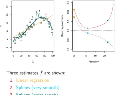
Figure 2.9. 0 20 40 60 80 100 2 4 6 8 10 12 X Y 2 5 10 20 0.0 0.5 1.0 1.5 2.0 2.5 Flexibility
Mean Squared Error
Three estimates fˆare shown:
1. Linear regression.
2. Splines (very smooth).
3. Splines (quite rough).
Red line: Test MSE.
Gray line: Training MSE.
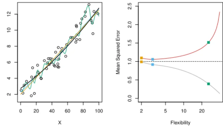
Figure 2.10 0 20 40 60 80 100 2 4 6 8 10 12 X Y 2 5 10 20 0.0 0.5 1.0 1.5 2.0 2.5 Flexibility
Mean Squared Error
The functionf is now almost linear.
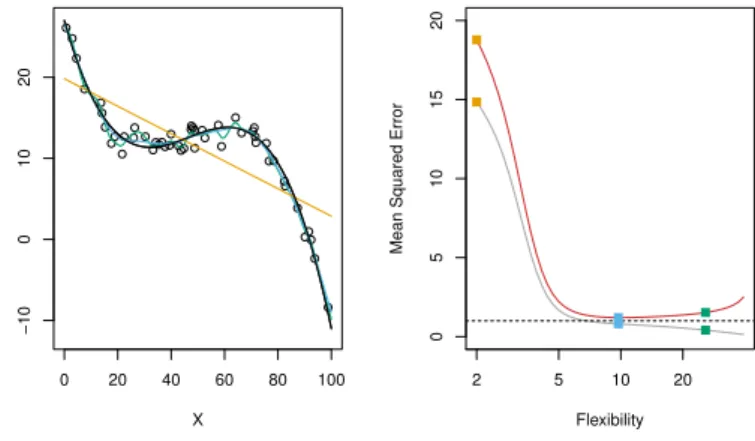
Figure 2.11 0 20 40 60 80 100 −10 0 10 20 X Y 2 5 10 20 0 5 10 15 20 Flexibility
Mean Squared Error
When the noiseεhas small variance, the third method does well. 14 / 24
The bias variance decomposition
Letx0 be afixed test point,y0 =f(x0) +ε0, and fˆbe estimated
fromn training samples(x1, y1). . .(xn, yn).
LetE denote the expectation over y0 and the training outputs (y1, . . . , yn). Then, the expected mean squared error(MSE) at
x0 decomposes into three interpretable terms:
E(y0−fˆ(x0))2 =Var( ˆf(x0)) + [Bias( ˆf(x0))]2+Var(ε0).
E(y0−fˆ(x0))2 =Var( ˆf(x0)) + [Bias( ˆf(x0))]2+Var(ε0). Irreducible error
E(y0−fˆ(x0))2 =Var( ˆf(x0)) + [Bias( ˆf(x0))]2+Var(ε0). The variance of fˆ(x0): E[ ˆf(x0)−E( ˆf(x0))]2 This measures how much the estimate offˆatx0
changes when we sample new training data.
E(y0−fˆ(x0))2 =Var( ˆf(x0)) + [Bias( ˆf(x0))]2+Var(ε0). The squared bias offˆ(x0): [E( ˆf(x0))−f(x0)]2
This measures the deviation of the average prediction fˆ(x0) from the truthf(x0).
Take-aways from bias variance decomposition
E(y0−fˆ(x0))2 =Var( ˆf(x0)) + [Bias( ˆf(x0))]2+Var(ε0).
I The expected MSE is never smaller than the irreducible error I Both small bias and small variance are needed for small
expected MSE
I Easy to find zero variance procedures with high bias (predict a constant value) and very low bias procedures with high
variance (choose fˆpassing through every training point) I In practice, best expected MSE achieved by incurring some
bias to decrease variance and vice-versa: this is the bias-variance trade-off
Rule of thumb
More flexible methods⇒Higher variance andLower bias. I Example: Linear fit may not change substantially with
training data but high bias if true f very non-linear
Squigglyf, high noise Linearf, high noise Squigglyf, low noise 2 5 10 20 0.0 0.5 1.0 1.5 2.0 2.5 Flexibility 2 5 10 20 0.0 0.5 1.0 1.5 2.0 2.5 Flexibility 2 5 10 20 0 5 10 15 20 Flexibility MSE Bias Var Figure 2.12 18 / 24
Classification problems
In a classification setting, the output takes values in a discrete set. For example, if we are predicting the brand of a car based on a number of car attributes, then the functionf takes values in the set{Ford, Toyota, Mercedes-Benz, . . .}.
We will adopt some additional notation:
P(X, Y) : joint distribution of (X, Y),
P(Y |X) : conditional distribution of X given Y, ˆ
yi:prediction of yi givenxi.
Loss function for classification
There are many ways to measure the error of a classification prediction. One of the most common is the 0-1 loss:
1(y06= ˆy0).
As with squared error, we can compute average test prediction error (calledtest error rateunder 0-1 loss) using previously unseen test data{(x0i, yi0);i= 1, . . . , m} : 1 m m X i=1 1(yi0 6= ˆyi0).
Similarly, we can compute the (often optimistic)training error rate 1 n n X i=1 1(yi6= ˆyi). 20 / 24
Bayes classifier
o o o o o o o o o o o o o o o o o o o o o o oo o o o o o o o o o o o o o o o o o o o o o o o o o o o o o oo o o o o o o o o o o o o o o o o o o o o o o o o o o o o o o o o o o o o o o o o o o o o o o o o o o o o o o o o o o o o o o o o o o o o o o o o o o o o o o o o o o o o o o o o o o o o o o oo o o o o o o o o o o o o o o o o o o o o o o o o o o o o o o o o o o o o o o o o o o o o o o o o o X1 X2 Figure 2.13In practice, we never know the joint probability P. However, we can assume that it exists. TheBayes classifierassigns:
ˆ
yi =argmaxj P(Y =j|X =xi)
It can be shown that this is the best classifier under the 0-1 loss.
K
-nearest neighbors
To assign a color to the input×, we look at its K= 3 nearest neighbors. We predict the color of the majority of the neighbors.
o o o o o o o o o o o o o o o o o o o o o o o o Figure 2.14 22 / 24