Analysis Guide
Version 2.0 for Microsoft Windows XP
0112-0170
September 2008
document is strictly prohibited, except as MDS Analytical Technologies may authorize in writing. Equipment that may be described in this document is protected under one or more patents filed in the United States, Canada, and other countries. Additional patents are pending.
Software that may be described in this document is furnished under a license agreement. It is against the law to copy, modify, or distribute the software on any medium, except as specifically allowed in the license agreement. Furthermore, the license agreement may prohibit the software from being disassembled, reverse engineered, or decompiled for any purpose.
Portions of this document may make reference to other manufacturers’ products, which may contain parts whose names are registered as trademarks and/or function as trademarks. Any such usage is intended only to designate those manufacturers' products as supplied by MDS Analytical Technologies for incorporation into its equipment and does not imply any right and/or license to use or permit others to use such product names as trademarks.
All products and company names mentioned herein may be the trademarks of their respective owners.
MDS Analytical Technologies makes no warranties or representations as to the fitness of this equipment for any particular purpose and assumes no responsibility or contingent liability, including indirect or consequential damages, for any use to which the purchaser may put the equipment described herein, or for any adverse circumstances arising therefrom.
For Research Use Only. Not for use in diagnostic procedures.
ISO
9 0 0 1
REGISTERED COMPANY
Equipment built by MDS Analytical Technologies, a business unit of MDS Inc. 1311 Orleans Drive, Sunnyvale, California, 94089 USA.
MDS Analytical Technologies is ISO 9001 registered.
© 2008 Edition MDS Analytical Technologies, a business unit of MDS Inc.
US C
METAXPRESS, METAMORPH, and IMAGEXPRESS are registered trademarks of MDS Analytical Technologies.
IMAGEXPRESSULTRA, IMAGEXPRESSMICRO, ACUITYXPRESS, ADAPTIVE ACQUISITION,
Chapter 1 Introduction . . . 5
Documentation Conventions . . . .6
Obtaining Support . . . .6
Chapter 2 Defining Analysis Criteria . . . 9
Chapter 3 Analysis Workflow . . . 11
Determining Analysis Settings . . . .11
Application Module Conventions . . . .12
Setting Application Module Parameters . . . .13
Chapter 4 Determining Settings for Analysis . . . 15
Settings in the Review Plate Data Dialog Box . . . .15
Chapter 5 Preparing For Analysis . . . 37
Automated Analysis . . . .37
Manual Analysis . . . .37
Using the Review Plate Data dialog box for Analysis . . . .37
Using the Plate Data Utilities Dialog Box for Manual Analysis. . . . .43
Chapter 6 Choosing Application Modules . . . 47
Determining what needs to be measured . . . .47
Chapter 7 Setting Up Application Modules . . . 51
MetaXpress® Application Module Configuration . . . .51
Running the Transfluor™ Application Module . . . .65
Viewing Analysis Results . . . .70
Transferring Data to an Excel Spreadsheet . . . .71
Cell-by-cell Multiplexing with Application modules in the MetaXpress® Software . . . .73
Chapter 8 Performing Automated Analysis . . . 75
General Procedure for Automated Analysis . . . .76
Chapter 9 Managing Plate Data . . . 83
Exporting Images. . . .90
Deleting Plates. . . .91
Deleting Images. . . .92
Deleting Measurements. . . .92
Chapter 10 Viewing and Understanding Analysis Results . . . 95
Extracting Results after Running your Analysis . . . .95
The MetaXpress® software workflow is divided into two major parts —
acquisition and analysis. The acquisition workflow involves configuring settings, acquiring images, and storing plate data in a database. The analysis workflow discussed in this manual consists of processing,
enhancing, and analyzing acquired plate data. Analysis can be performed using the following methods:
• AutoRun — Automatically start application modules or custom journals to run on plates as soon as they are acquired. This can be done over a network using dedicated analysis machines or locally.
• Manual — Manually run application modules or custom journals on plates already stored in your MDCStore™ database and/or File
server.
• Batch Analysis — Manually add analysis jobs on plates stored in your MDCStore database and/or File server to the AutoRun queue.
The following topics are discussed in this guide:
• Identifying and using Online Help, PDF Documentation, Web-based Documentation, and Support resources.
• Determining the image quality requirements for your experiments
• Viewing your images
• Viewing different wavelengths in one image or multiple images
• Changing the display options of an image
• Using MetaXpress Application Module procedures to: Define application module settings
Note: You can also use the AcuityXpress cellular informatics software to further analyze your data.
Note: For more information about the MetaXpress acquisition workflow, refer to the “Acquisition guide” for your hardware platform.
Review plate data
Store plate data into your database Export data to Excel/text file
• Importing images into the database
Documentation Conventions
Before you begin using the MetaXpress® system, familiarize yourself with
the stylistic conventions used in this manual:
Obtaining Support
Part of effective communication with MDS Analytical Technologies is determining the channels of support for the MetaXpress® application.
MDC provides a wide range of support materials that should be your first step when troubleshooting problems. Please complete the following steps in order when attempting to resolve any MetaXpress issues:
1. Consult the Documentation — Check the manuals that shipped with the system, as well as the online help available within the MetaXpress® application. Press F1 to access the online help for an
active dialog box. In the Help window, click See Also to view and choose from a list of related topics.
Table 1-1 Document Conventions
Bold type Indicates a chapter or section heading, or is used for emphasis Courier
font Indicates the name of a file or folder, the output of command, or text that you must type Italic type Indicates the name of a command or field, or text from a field,
2. Explore the MetaXpress Literature website for application notes — http://www.moleculardevices.com/product_literature/family_links. php?prodid=114.
3. Explore the Molecular Devices Support website — The support site, located at
http://www.moleculardevices.com/pages/support.html has links to technical notes, software upgrades and other resources. If you do not find the answers you are seeking, follow the links to the Technical Support Request Form.
4. Internet Support — Fill out the Technical Support Request Form at http://www.moleculardevices.com/cgi-bin/support_request.cgi to send an e-mail to a pool of technical support representatives. 5. Call Customer Service — Contact Customer Service at
(800)-635-5577 (U.S. only) or +1 408-747-1700. Please have the system ID number, system serial number, software version number and the system owner’s name available when you call.
Additional support resources include the following: Nikon web-based microscopy course —
http://www.microscopyu.com The Molecular Probes handbook—
http://www.probes.invitrogen.com offers advice on fluorescent probes and help determining if there are better stains
available for your analysis.
The following sites offer filter information: http://www.chroma.com
http://www.semrock.com http://www.omegafilters.com
When preparing to analyze plates, consider the following plate characteristics:
• Plate Specifications – How many wells on the plate?
Plate size is a determining factor in the number of images included in the experiment. Experiments containing large numbers of images will need more time to be analyzed than ones from smaller experiments. Factors like this might influence the options and settings that you choose for your analysis.
• Wells – Were images acquired from all wells?
Your plate might contain images for all wells, but because of the requirements of your experiment, you might not want to analyze all wells on all plates.
• Sites – How many sites were acquired for each well?
The number of sites acquired for each well can influence how to analyze the data and organize your analyzed data for review. Since the number of sites value applies to all wells from which you are acquiring data, the quantity of data collected is multiplied by the number of sites visited in each well.
• Wavelengths – How many wavelengths and which specific wavelengths were acquired?
Similar to sites, the number of wavelengths acquired contributes to the amount of data acquired from each well. Some application modules require a minimum number of wavelengths to be
acquired in order to produce meaningful data, while other
modules will produce good results with only a single wavelength.
• Images – What is the total number of images acquired on the plate?
The total number of images that you acquire is influenced not only by the number of wells that you acquire, but also the number of time points, the number of wavelengths for each time point, and the number of sites in each well. Therefore, the potential exists for creating very large data sets. Keep in mind that the amount of time available to process your data can become an important
• Settings – What unique analysis settings do you need to make? Each available application module is linked to a settings file that you can access from the application module dialog box. After you store your settings, you can recall and reuse these settings at any time. Saving and reusing your settings enables you to streamline your experiment workflow and ensure a high level of consistency and accuracy.
• View Characteristics – What viewing characteristics do you want? The viewing characteristics that you choose on the Review Plate Data Display tab enable you to enhance the appearance of up to three wavelengths. You can view these wavelengths in separate image windows or you can click Color Composite to combine the images into a single overlay, composite image. You can also choose to display the well number on the image as well as the value that is shown for each well or site on the table.
• Expected Results – What are the anticipated results of your experiment?
The results that you expect to obtain from your experiment can be one of the best guides in helping to properly design your
experiment. By “working backward” from your anticipated results, you can ensure that you correctly identify all of the steps needed to design a successful experiment.
• Data Log Measurement Selections – Which measurements are the most appropriate to select for logging?
Most MetaXpress® application modules create two different types
of logs: a Summary log and a Data log. Summary log
measurements are measurements that apply to the entire image and include a number of default measurements that apply to every image. Data log measurements are also referred to as cell-by-cell measurements. These measurements are logged for each
individual cell in the image that has been identified by the software. Some application modules have High Throughput (HT) versions. Because of the increased throughput, these modules log only summary measurements and not cell-by-cell measurements.
Analyzing image data with the MetaXpress® software involves using
several dialog boxes and toolbars in sequence to create a workflow. Most of these dialog boxes are located in the Screening and Apps menus. This chapter provides an overview of how to use these tools to configure analysis and explains the common conventions used by the MetaXpress application modules.
MetaXpress application modules are software modules designed to automate analysis procedures such as segmentation and cell scoring. Application modules, along with user-defined journals and manual analysis, make up the methods available to create an effective workflow. For more information, see Chapter 6.
Note that after you design a workflow, you can further automate the process by creating custom MetaXpress tool bars and task bars. For more information on custom MetaXpress tool bars and task bars, refer to the
“Acquisition Guide” for your hardware platform.
Determining Analysis Settings
Complete the following procedure to determine the best settings to analyze your plate image data:
1. In the Review Plate Data dialog box, locate and select the plate of interest. For information on the Review Plate Data dialog box, see
Using the Review Plate Data dialog box for Analysis on page 37. 2. Set viewing characteristics to improve the visibility of information. 3. Determine the analysis process to use – prepared application
modules or custom journals.
4. Determine the settings needed. For specific instructions on performing manual analysis for the purpose of running a trial analysis, see Chapter 7.
Note: This procedure is a broad overview and assumes you know how to open images from the Review Plate Data dialog box. For instructions on using the Review Plate Data dialog box, see Chapter 5.
Examine and evaluate the initial results.
Adjust settings to correct for inaccurate results. Repeat process until good results are obtained.
Prepare to run automated analysis. For information, see
Chapter 8.
Application Module Conventions
Most MetaXpress® application modules share similar configuration steps,
such as selecting images to process or determining an object’s width. An understanding of these similar steps helps when learning to use different application modules. The following capabilities and conventions are shared across most of the MetaXpress application modules:
• Principles of Segmentation — Image segmentation is the process of spatially partitioning an image into meaningful objects.
Generally for fluorescent imaging, objects are bright and are segmented from a darker background. Additionally, segmentation may include the automatic splitting of touching cells or objects to give a more accurate count.
• Adaptive Background Correction™ (ABC) process — The system
automatically corrects uneven image backgrounds throughout the image by adapting to local content. This allows for more robust segmentation and image analysis repeatability. The ABC process is used solely for defining object boundaries and is not used to modify reported intensity measurements. Intensity measurements such as Average Intensity and Integrated Intensity come directly from the original pixel data unless otherwise indicated.
• Size Parameters — The modules all require that the user supply an approximate size or range of sizes for the desired object
detection. These values help to fine-tune automated algorithms that analyze objects according to the biology of the application. Appropriate values can be determined using the software’s
Note: Some modules, such as Translocation-Enhanced, indicate that an overall constant background intensity value can be uniformly
subtracted from all pixel intensities during measurement. However, this uniform subtraction is completely independent of the ABC
interactive Region Tools applied directly to the image being analyzed.
• Intensity Parameters — The modules all require that the user supply an Intensity above the local background detection parameter. This parameter specifies the minimum intensity level needed to detect the presence of a fluorescent stain and can be used to adjust the sensitivity of the detection. Since the ABC system adjusts for uneven background, these values are taken locally for each object detected, relative to local background levels, rather than on a global absolute basis.
Setting Application Module Parameters
Before you can use a MetaXpress® application module effectively, you
must make settings in the application module dialog box based on the properties of the image or images that you are analyzing.
Depending on the dialog box, most of the modules have three to five major areas that contain controls. The following settings are used in most or all of the MetaXpress application module dialog boxes:
Stained area — This drop-down list box enables you to apply your measurement to only the nucleus, only the cytoplasm, or both.
Approximate minimum width — This measurement specifies the smallest object that you want to detect.
Approximate maximum width — This measurement specifies the largest object that you want to detect.
Intensity above local background — This value is used to adjust the sensitivity of detection to effectively delineate objects from the background. Since even background values within an image are common, the software automatically accounts for unevenness using the ABC system and compares intensities relative to local background rather than a single global value.
Note: For information on configuring application modules, see
Settings for analysis are made in the following dialog boxes:
• Review Plate Data dialog box
• Application module dialog boxes
Settings made in the Review Plate Data dialog box define the overall characteristics of your analysis. These settings are used to adjust the view of existing data and to select data for analysis. They do not affect image analysis or other measurements and cannot be saved and reused.
Settings made in application module dialog boxes define setting
characteristics specific to the selected application module. These settings can be saved and reused.
Application module dialog boxes can be accessed either through the Review Plate Data dialog box, or directly through the Apps menu. When you begin to make your settings, determine whether you will be
modifying an existing group of settings or creating completely new settings.
Settings in the Review Plate Data Dialog Box
You can configure settings in the Review Plate Data dialog box only after you have selected a plate for analysis. For more information, see
Preparing For Analysis on page 37 for selecting and loading a plate from your database.
Settings on the Review Plate Data dialog box are primarily made on the four tabbed areas of the dialog box. Since settings made in the Review Plate Data dialog box are simply for looking at the data, they cannot be stored in a setting file to be used again in the future.
From the Run Analysis tab of the Review Plate Data dialog box, you can select and access individual application module dialog boxes. Settings for application module dialog boxes can be saved to a settings file that is specifically used by that application module and can be saved and recalled for future use.
The following section lists and describes each of the available dialog box options on the main dialog area and the four tabs of the Review Plate Data dialog box. You should become familiar with these settings and their
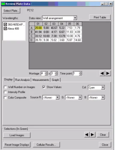
Figure 4-1 Review Plate Data dialog box – Analyzed plate open
Select Plate: Opens the Plate Dialog box. Use this dialog box to select Plate Data Sets of stored microwell plates from the database for viewing. To perform other operations, such as deleting plates or individual images, use the Plate Data Utilities dialog box.
Data view: Selects and indicates the well arrangement as shown in the Microplate Selection Grid and the Image Montage window.
Well arrangement: Organizes your viewable images in the Image Montage window in the layout in which the wells are presented in the microplate.
Well vs measurement: Compares wells against the available measurements.
Print: Prints the data in the table on the selected windows printer. Wavelengths: Determines whether or not images from available wavelength will be displayed.
Sites: Selects one or all the sites in each selected well in your experiment. Available sites are indicated by a dash. Click on any available site to view only that site for all selected wells in the thumbnail view. Click All Sites to view all sites for all selected wells. If you run an Analysis on wells with sites, the values displayed in the table refer to the selected sites or, if All Sites is selected, the average for the total number of sites in the well.
All Sites: Specifies that all sites for all wells are to be included in each thumbnail image, and that each image in the thumbnail will be
represented as an individual image in the image selection grid for the Montage. However, the number of sites shown in both the thumbnails in the Montage and in the image viewer also depends on the Montage dimensions that you specify. When this box is checked, the sites in the well are included in the Montage dimensions. For example, if each well has four sites, and the Montage dimension is 1X1, only the upper left site in well A01 is shown; if you change the dimension to 2X1, the two upper sites are shown. Only when the dimension is set to 4X4 are all four sites in A01 shown. If this box is not checked, only a single, selected site is shown in the Montage, and each selection box in the image selection grid represents all sites for each well. Therefore, when not checked, when you select a different site in the Sites box, both the thumbnail in the montage and the image in the image window will be updated.
Microwell Plate Selection Grid: Indicates the wells containing image data, the images included in the Montage, and the images selected for display.
Montage: Specifies the dimension in image thumbnails of the Image Montage window.
Note: Image Montage windows are labeled as HTS- followed by the name of the stain or wavelength that you assigned to the wavelength. For example, HTS-DAPI or HTS-FITC.
Time Point: Specifies the number of timepoints that you want to display and/or include in the image montage.
Selections (In Green): Controls the selection and loading of images that you selected in the table. Select images by right-clicking on an image selection box, or by right-clicking on the associated image in the thumbnail view.
Load Image(s): Loads the images you selected in the table into a stack for each wavelength, or a single stack if Color Composite View is selected. Each of the three available data views, Well Arrangement, Time vs well, and Measurement vs Well, can be selected and used to generate an image stack, providing three different types of image stack results.
Arrow Buttons: Changes the displayed selected image to the previous or next selection (Selections [In Green]).
Clear: Clears all Selections from the table.
Reset Image Displays: Resets the view settings in all image displays. Cellular Results: Opens the Cellular Results dialog box. Use this dialog box to view and browse available analysis measurements. These
measurements are configured in the Configure Settings>Configure Data Log (Cells) dialog box.
Close : Closes the Review Plate Data (DB) dialog box. Reviewing Plate Data
To view and analyze images from a plate acquisition, complete the following procedure:
1. From the Screening menu, click Review Plate Data. 2. In the Review Plate Data dialog box, click Select Plate.
The Plate dialog box opens, and the Review Screen Data dialog box temporarily closes.
Note: The results shown are those from the analysis selected on the Measurements tab.
3. Expand the plates folder in the top pane of the dialog box to view folders containing plates saved in the database.
4. Double-click a folder to view its contents in the lower pane. 5. Select the plate containing the data to view and click OK.
The Plate dialog box closes, and the Review Screen Data dialog box reopens.
6. In the Wavelengths field, clear the checkboxes for each wavelength to initially inhibit the display of images for each wavelength.
7. In the Data view drop-down list, select the type of view that you want to use:
Well arrangement — Arranges your viewable images in the montage in the order in which the wells are presented in the microwell plate.
Time vs Well — Compares timepoints against wells or well selections.
Measurement vs Well — Compares wells against the available measurements.
8. Using the table features, define the wells that you want to view. You can view “thumbnails” in a montage of images and select the size of the thumbnail images. You can select images from the Montage and view each image separately in an image window. You can select images from anywhere in the table, and load the images into a stack.
To define the images that you want to include in the thumbnail view, type or select an area of number of wells in the Montage boxes.
Click Apply to implement the number of Wells and Timepoint settings that you made.
Click either the left or right arrow to move thumbnail selector left or right in the table.
OR
Click anywhere on the table to place the first selection box at that location.
To load images into a stack, right click on the squares for the images that you want to include in the stack, then click Load Image(s) in the Selections [In Green] section.
Click either the left or right arrow in the Selections [In Green] section to open a full image view and/or to change the view to the next or previous selected image. The image currently displayed in the image view is indicated by yellow highlight. Click on an image in the montage to see full resolution of the
displayed image. You can make measurements on the images as they are displayed.
Click Clear to remove all Selections [In Green] from the table. 9. Click the Display tab to set display options applicable to the
analysis you will run.
10.Click the Run Analysis tab to specify settings for running your selected analysis.
11.Click the Measurements tab to specify measurement criteria for your selected analysis, as required.
12.Click the Graph tab to configure a graph for the data.
13.Click Reset Image Displays to reset any open image displays to the default values.
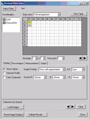
14.Click Close to close the Review Plate Data dialog box. Display Tab Settings
The settings on the Display tab do not affect your analysis results. These setting are used to improve the visual appearance of the images on your plate, and to add additional information to the display, such as the well number and certain analysis values. It also enables you to generate an intensity profile to help you determine the areas of the image that have the highest intensity.
Note: The Measurements tab is used to view images for which an appropriate analysis has already been run. Each measurement included in the application module log file can be viewed interactively. Use the Well Selection option to choose the wells that you want to view.
Figure 4-2 Review Plate Data dialog box – Display tab
Show Values: Displays average Analysis values on the table and in the upper right corner of each image in the montage if Show well information is selected under Image Overlay. For each site, the values shown both on the table grid and the montage display are the average of all the values for all defined objects in the site. To see individual values for identified objects, click Cellular Results. The Cellular Results dialog box will open and display a table of values for all objects in the selected well or site.
Image Overlay: Overlays information onto thumbnails in the Image Montage and onto individual images for each selected wavelength. The following selections are available:
No overlay display — No data is overlaid on the image. Show well information — The data for the measurement
selected on the Measurements tab is overlaid on the image. Show cell segmentation — The segmentation image
generated by the application (if available) is overlaid on the image.
Col: Selects text color to apply to well numbers and values displayed in the image.
Intensity Profile: Transforms the image into a three-dimensional intensity profile graph, using the colors assigned to the image and assigning the highest intensities to the highest peaks in the graph.
Color Composite: Creates a single color composite of two or three wavelengths based on the colors (R/G/B) that you assign to the wavelengths in the Source boxes.
Source (R, G, B): Assigns one or more of the primary colors to one or more of the wavelengths that you are using in your experiment.
Scale 16-bit Images: Enables you to apply scaling to 16-bit images either automatically or manually when color composites of intensity profile images are created. If source images are displayed, then their scaling can be set through the scale image dialog.
Range: Assigns the upper limit of the 16-bit scaling range when using manual scaling for 16-bit images. This box is inactive when Auto Scale is checked.
To configure the display settings for the Review Plate Data dialog box
1. In the Image Overlay drop-down list, select one of the following selections:
No overlay display — No data is overlaid on the image. Show well information — The data for the measurement
selected on the Measurements tab is overlaid on the image. Show cell segmentation — The segmentation image
generated by the application (if available) is overlaid on the image.
Note: This enables the Scale 16-bit Image fields that are described under Scale 16-bit Images in the following paragraphs.
Note: It is recommended that you do not activate Color Composite before you have configured your settings as it prevents images from updating while you are making your configuration settings.
2. In the Col drop-down list, select a text color for the Well Number and/or the measurement values overlaid on the image.
3. Select the Intensity Profile check box to transform the image displayed into a three-dimensional intensity profile graph.
4. Select the Color Composite check box to combine images for two or three wavelengths into a single image using the color
assignments in the Source R/G/B drop-down lists.
5. If the Intensity Profile and/or Color Composite check box is selected, select the Auto Scale check box to turn on auto scaling for 16-bit images, or clear to turn off auto scaling and manually specify the scaling range.
6. If the Intensity Profile and/or Color Composite check box is selected, and Auto Scaling is off, select the appropriate scaling range in the Range drop-down list.
Run Analysis Tab Settings
The settings on the Run Analysis tab are used to choose the application module or journal that you want to run, select the setting file to be used during the analysis, and to run the analysis on either the entire plate, the selections that you made previously in the well selection grid area, or the currently selected site.
This tab also enables you to open the Edit List of Settings dialog box for a specific application module or journal and choose the setting file that you want to use, modify an existing setting, create a new setting file, or delete a setting file.
Analysis: Selects and indicates the name of the analysis that you are running. This can be either a prepared analysis, such as Neurite Outgrowth, or analyses created from journals.
Settings: Selects and indicates the settings name from the available settings associated with the analysis that you are using. Use the Configure Settings button on this tab to make different settings available for use with your selected Analysis.
Edit List: Opens the Edit List of Settings for <Neurite Outgrowth> dialog box. The Edit list of Settings for dialog box is used to edit settings applied to application modules included in the MetaMorph® software, such as
Neurite Outgrowth. Analyses that you create from journals must have all possible settings stored in the database at the time the journal is created and stored in the database C:\Assay folder.
Description: Displays one of the following types of descriptions. For application modules that are MetaMorph Drop-ins, such as Neurite Outgrowth, this area displays the same description as the Meta Imaging Series Administrator Configure Drop-in dialog box displays for the module. For analyses defined by journals, it displays the description information typed into the Analysis Description area when the analysis was added to the database.
Log into the database: Opens the database login dialog box if you are not logged in when you run the analysis.
Base Result Folder: Enables you to select the location within the database where the results data from the application module is stored. Configure Settings: Opens the Configure settings for <Neurite Outgrowth> dialog box or the associated dialog box for the selected application module. This option is only available for application modules. Analyses created from journals must be configured in the originating journal.
Run Setup for Analysis: Runs the setup journal for the selected analysis if it exists. The setup journal must be in the same folder as the main analysis and must be named in the format: EXAMPLEJOURNAL_SETUP.JNL.
Note: This option is only available if the selected analysis is created from a journal and not a prepared analysis like Neurite Outgrowth.
Run Analysis for All Positions: Runs the analysis for all wells that are indicated to contain a sample. Wells containing valid samples are indicated by a dash in the grid location for the well.
Run Analysis for Selections: Runs the analysis for all selected wells. Right-click on a well to select it. Selected wells are indicated by a green rectangle.
Run Analysis for Site: Runs the analysis for just the selected and displayed image site.
To run an application module or an analysis created from a journal
1. In the Review Plate Data dialog box, click the Run Analysis tab. The Run Analysis tab moves to the front.
2. In the Analysis drop-down list, select the analysis that you want to run, or use the prefilled selection.
3. If you are using the default settings of a MetaXpress® application
module, such as Neurite Outgrowth, or a custom analysis derived from a journal, go to Step 10.
4. In the Settings drop-down list, select the setting that you want to apply to the analysis, if more than one selection is available. 5. If you need to modify the configuration of an application module
such as Neurite Outgrowth, click Configure Settings. The dialog box for the application module opens.
6. If you need to add another setting to an existing application module, click Edit List.
7. In the Edit List of Settings for <Neurite Outgrowth>, click New Settings.
8. In the New Settings for <Neurite Outgrowth> dialog box, type a name in the Name field, then click OK.
The Configure Settings for Neurite Outgrowth dialog box opens. This is a special version of the Neurite Outgrowth dialog box
Note: The following procedure uses the Neurite Outgrowth application module as an example of how to use this tab.
specifically for defining new settings for your Neurite Outgrowth application module.
9. Use the help information for Neurite Outgrowth to make the appropriate settings changes, then click Close.
10.Select the Log into the database check box to log the measurement data from your analysis into the database.
11.If you are running a custom analysis derived from a journal and have created a setup journal for it, click Run Setup for Analysis to run the setup journal.
12.To select a database location for your analysis data, select Base folder for results.
13.In the Measurements Sets dialog box, select the Measurements Sets folder and click OK.
All measurement data from your analysis will be stored as a subfolder under this folder.
Note: To access Help associated with a specific dialog box, press the F1 key when the dialog box is active. When the Help window opens, click See Also to view and select from a list of procedures and dialog box options.
Note: This step is necessary only the first time you run the analysis.
Note: Measurement sets and subfolders can be moved and renamed from within the AcuityXpress software as needed.
14.If you are running the analysis for all wells and all defined sites in the database, click Run Analysis for All Positions.
15.To run your analysis for only the selected wells, click Run Analysis for Selections.
16.To run your analysis for a specific site, select the site, and then click Run Analysis for Site.
Measurements Tab Settings
The Measurements tab enables you to select and view a previously run analysis and choose a single measurement from the analysis to view within the montage window and the well selection grid area. It also enables you to select wells for viewing based on a variable value range that you specify in Select Wells Based On Variable Range. Values can be logged in a typical log file, such as an Excel Spreadsheet or a text file.
Figure 4-4 Review Plate Data dialog box – Measurements tab
The Review Plate Data (DB) Measurements Tab enables you to query the database for specific measurements that fall within your specified limiting range.
Analysis: Selects the completed analysis that contains the measurements to extract.
Measurement: Selects a single measurement to use for querying
measurement data stored in the screening database. Click the down arrow to open the list of available measurements. The list of measurements can vary for each image or for each experiment’s group of images. The selected measurement will be displayed in the data table when Well
Arrangement or Time vs Well is selected. The selected measurement will also be displayed in the show values on the montage when appropriate. Display Format: Specifies the number of decimal places to be included in the result data. The display format selection can vary depending on the type of measurement selected.
Select Wells Based on Variable Range: Specifies the range within which you want to run the query for the measurement that you selected.
Value is: Selects and specifies the query qualifier. Qualifiers are equals (=), greater than (>), less than (<), between, outside, or like.
Select: Runs the specified query and selects all wells or sites that fall within the query requirements.
Configure Log: Configures the open log file. Opens the Configure Log dialog box. Select Column and Row labels, and /or Plate info, or neither. Open Log/Log Data: Opens the Open Data Log dialog box. Choose to log measurements to either a Dynamic Data Exchange (DDE), a text file, or both. After you have opened the log file, this button becomes Log Data. The data in the table of this dialog box is logged to the destination(s) that you selected.
To specify well selection based on specified measurements query criteria
1. In the Review Plate Data dialog box, click the Measurements tab. The measurements tab moves to the front.
Note: The data in your table is logged locally to your selected destinations and not to the MDCStore database.
2. In the Analysis drop-down list, select the analysis that contains the measurements to query.
3. In the Measurement drop-down list, select the name of the measurement that you want to use to query your images in the database.
4. In the Display Format drop-down list, select the number of decimal places that you want to display in the grid.
5. In the Value is drop-down lists, select the variable range limit specifier and the numerical value(s) of the range.
6. Click Open Log to open either a Dynamic Data Exchange or a text log file, then click OK.
7. Click Configure Log to select either Column and Row labels, Plate info, or both, and then click OK.
8. Click Select to query the image database using your selected measurement and variable range limits.
The selected wells or sites will be highlighted in green. 9. Click Log Data or press F9 to log your query data. Graph Tab Settings
The Graph tab enables you to create a graph for a single Application Module analysis or a single Journal analysis. You can specify that the graph view include the entire plate, that it consist of multiple graphs of displayed wells, or that it is for a single, selected well. Make your well choices in the Montage window, then choose the graph type and measurements.
Note: Additional options for visualizing your image analysis data are available in the AcuityXpress software.
Figure 4-5 Review Plate Data dialog box – Graph tab
Analysis: Selects the completed analysis that contains the data to graph Graph View: Determines the source of the data plotted in the graph. Valid options include the following:
Plate: Graphs the summary well measurement for all the wells in the plate. Select this option to view the data for an entire plate.
Multiple graphs of displayed wells: Displays separate graphs for each well displayed in the montage. If you change the appearance of the graph using the Graph Settings dialog box, each mini-graph is updated.
Single Well: Graphs all values of a measurement within a well.
Graph Type: Determines the type of data and how it is displayed for the graph. The choices available depend on what is selected in the Graph View field. The following options are available for each Graph View option:
Plate
Histogram— Displays a bar chart, in the format of
Measurement (Area, Correlation, Coefficient, etc.) vs. Count. Measurements vs Well Column — Displays a graph with one
trace for each column of the plate, in the format of
Measurement (Area, Correlation Coefficient, etc.) vs. Column. You can view the data as one trace with error bars by clicking the Down Arrow button directly below the left side of the graph and selecting Show Mean with Error Bars from the drop-down menu.
Measurements vs Well Row — Displays a graph with one trace for each row of the plate, in the format of Measurement (Area, Correlation Coefficient, etc.) vs. Row. You can view the data as one trace with error bars by clicking the Down Arrow button directly below the left side of the graph and selecting Show Mean with Error Bars from the drop-down menu.
Measurements vs Well Number — Displays a graph with one trace for each well number in the format of Measurement (Area, Correlation Coefficient, etc.) vs. well number. The well number is calculated as follows:
Well number = Current Column + (Current Row * Number of Columns)
Scatter Plot— Displays a scatter plot graph containing two measurement variables for the plate.
Multiple Graphs of displayed wells:
Time— Displays multiple graphs of the selected wells in the format of Measurement (Area, Correlation Coefficient, etc.) vs. time point number. If the selected measurement is not
recorded at specific time points, but applies to all data, the trace will be flat. If the value is only recorded at some time points, only those time points will be used in the graph. Single Measurement—Displays a bar graph for each of the well
in the montage view. If the Data View field is set to Measurement vs Well or Well Arrangement, then the
measurement shown is taken from the time point indicated in the Time Point field. If the Data View field is set to Time vs Well, then the graph shows the measurement for each time point that is shown in the montage.
Measurement Pair—Displays a bar graph for each of the selected wells that contains data for two Measurement selections.
Single Well:
Time— Displays a graph with one trace for each cell, in the format of Measurement (Area, Correlation Coefficient, etc.) vs. Time Point.
Histogram— Displays a bar graph of the counts of values sorted into bins.
Scatter Plot— Displays a scatter plot graph containing two measurement variables (Area, Correlation Coefficient, etc.) for each cell in the well.
Measurement: Selects the measurement to be graphed. The options available are extracted from the active experiment and include all numerical data measurements configured in the application module or analysis. The y-axis is autoscaled to contain the measurement data selected in this field.
Measurement2: Selects the second measurement option when available. The range of this data is used to scale the x-axis in both scatter plots and measurement pair graphs.
Number of Bins: Selects the number of bins use when creating the histogram. This option is only available when Histogram is selected from the Graph Type field.
Auto Scale: Automatically scales the bins based on the range of data from the selected Measurement. This option is only available when Histogram is selected from the Graph Type field.
Scale Min/Max: Manually selects the minimum and maximum range for histogram based on the data in the Measurement field. This option is only available when Histogram is selected from the Graph Type field and Auto Scale is not checked.
Set Display to Default: Sets the display parameters for the current graph to its default. There are separate graph defaults for each combination of Graph View and Graph Type.
Show Graph: Opens the graph using the current settings. If a graph is already open and the settings are changed, Show Graph will update the open graph.
To display screen data on a graph
1. In the Review Plate Data dialog box, click the Graph tab. The Graph tab moves to the front.
2. Select the data from the Analysis drop-down list.
3. In the Graph view section, select the source location for the data. 4. Select a graph type from the Graph type drop-down list.
5. Select the measurement(s) from the Measurement and Measurement2 (if applicable) drop-down list(s).
6. If Histograms is selected in the Graph type drop-down list, select the number of bins to display in the resulting histogram in the Number of bins list.
7. Select the Auto Scale check box to automatically scale the bin(s) based on the range of data from the selected Measurement.
8. Click Show Graph to open the graph based on the current settings
.
9. To configure the graph settings, double-click inside the graph or click the arrow on the bottom left corner of the graph and click Graph Settings. For examples of graphs, see Graph Examples on page 33.
10.To set the display parameters to the default view, click Set Display to Default in the Review Plate Data dialog box.
There are separate graph defaults for each combination of Graph View and Graph Type. For examples of graphs, see Graph
Examples on page 33. Graph Examples
The following graphs are examples of the types of graphs that you can
Note: The options available for each graph type vary depending on the Graph View setting.
Note: This option is only available when Histogram is selected from the Graph type drop-down list.
Note: If the data on the graph is not displaying properly, click and drag one of the corners of the graph window to resize it.
Figure 4-6 Histogram – Number of Cells (Count) versus the Percent of Cells of Significant Growth
Figure 4-7 Measurement versus Well Column – Percent of Cells of Significant Growth versus Column
Figure 4-8 Measurement versus Well Row – Percent of Cells of Significant Growth versus Row number
Figure 4-9 Measurement versus Well Number – Percent of Cells of Significant Growth versus the Well Number
Figure 4-10 Scatter Plot – Total Cell Body Area versus the Percent of Cells of Significant Growth
There are two methods available to analyze acquired data — automated and manual. This chapter provides an overview of each, then explains how to use the Review Plate Data dialog box to manually open data for review. For information on the complete procedures, see Chapter 7, and
Chapter 8.
Automated Analysis
The first opportunity to run a selected analysis on a plate is in conjunction with the acquisition of your plate image data. If analysis of the plate has been scheduled, automated analysis will begin after the acquisition of the last well. For information on how to initiate automated analysis, see
Chapter 8. With automated analysis, a single application module or journal set can be used to complete your analysis. Image data is retrieved from the MDCStore™ database and analyzed; the analysis results are
subsequently stored back in the MDCStore database.
Manual Analysis
In most circumstances, in spite of the automated capabilities, you still should run manual preliminary tests on one or more wells to set the necessary dialog box options and settings needed to obtain valid results. After you determine effective settings for your experiment, you can store the settings for future use.
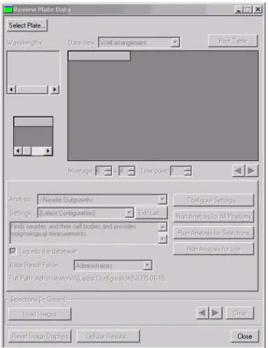
To begin manual analysis of images already stored in your database, open the Review Plate Data dialog box from the Screening menu. The Review Plate Data dialog box enables you to configure settings for preparing for and conducting manual image analysis. You can open this dialog box without having any plates open.
Using the Review Plate Data dialog box for Analysis
1. From the Screening menu, click Review Plate Data.When you open the Review Plate Data dialog box without any plates open, it will appear as shown in Figure 5-1.
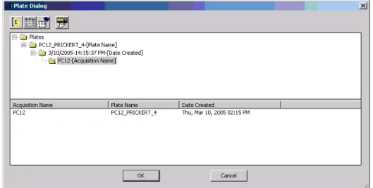
2. Click Select Plate to open the Plate dialog box and select one or more plates to analyze.
Figure 5-2 Plate Dialog with a plate selected
3. In the Plates folder, locate the plate that you want to analyze, and double-click the plate name.
The name of the plate and its associated attributes appear on the lower part of the Plate Dialog window.
4. Select the plate in the lower part of the Plate Dialog window and click OK.
The results of your query open in the Review Plate Data dialog box.
Figure 5-3 Review Plate Data dialog box with plate loaded for analysis
Plate Dialog Box Options
The buttons on the top of the Plate dialog enable you to configure how the plate data is displayed:
Figure 5-4 Plate Dialog options
Configure Plate Query
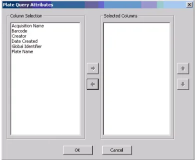
The first button is the Configure Plate Query button. This button opens the Plate Query Attributes dialog box shown in Figure 5-5.
Figure 5-5 Plate Query Attributes window
This dialog box lists available query attributes in the Column Selection field.
Note: If you place the cursor momentarily on a button, a tool-tip opens describing or naming the button.
To create a query
1. Highlight the attributes to include in your query, and click the right-facing arrow.
The attributes will be moved to the Selected Columns filed. 2. Use the up and down arrows to arrange the query sort order.
For example, if you want the primary sort to be based on all available users, place Creator at the top of your Selected Columns list. Then if you want to find all plates created on a specific date for each user, place Date Created next on the list. Finally, if you want to find all plates assigned to a specific acquisition name, place Acquisition Name as the last entry in your query list.
Initiating a Query
To initiate the query, click the Retrieve Data button or double-click the plate name in the query list. The name of the plate appears in the plate area:
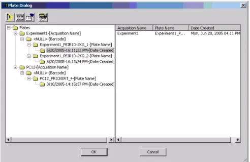
Changing from Horizontal to Vertical Arrangement
The default arrangement for the Query Select and Query Result in the Plate Dialog window is horizontal. To change from a horizontal to a vertical configuration, right-click inside either window area and click Vertical Arrangement.
Figure 5-7 Plate Dialog menu
Figure 5-8 Plate Dialog showing query retrieval results in the vertical arrangement
Using the Plate Data Utilities Dialog Box for Manual
Analysis
Use the Plate Data Utilities dialog box to run analysis on more then one plate at a time.
Figure 5-9 Plate Data Utilities dialog box
2. Click Run Analysis.
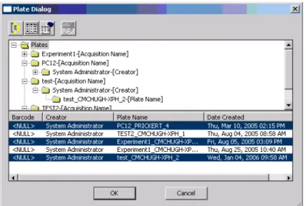
3. In the Plates Data dialog box, you can initiate analysis on multiple plates. Use the Query tools or manually select a node so several plates open in the bottom window. Press Ctrl, and click to select multiple plates.
Figure 5-10 Plate Dialog with multiple plates selected
Figure 5-11 Run Analysis on Plates dialog box
5. In the Run Analysis on Plates dialog box, select the analysis, settings, and the results folder for the selected plates. 6. Select one of the following from the Run method section:
Run now on this computer — Runs all selected analyses on the computer being used.
Add to auto run list — Adds the selected analyses to the Auto Run queue.
7. Click OK to start the analysis for the selected plates.
Note: For information on performing analysis, see Chapter 5, and
Molecular Devices offers optional MetaXpress® application modules that
automate common analysis tasks such as segmentation and cell counting. These tasks can be run from the Review Plate Data dialog box, opened as a stand alone dialog box, or used within a custom journal. These tasks can also be scheduled to run automatically in conjunction with the plate acquisition process.
This chapter describes several common analysis tasks and recommends application modules that help automate the tasks. Many of the modules share common conventions and settings. An understanding of the
general principles of using application modules enables you to use any of these modules by referring to the associated online help or this
document.
Determining what needs to be measured
Consider what needs to be measured by your assay. Your assay might encompass activation of a receptor, apoptosis, and proliferation and so on, but to obtain meaningful numerical data from screening, you need to describe a phenotype that can be measured by the imaging system. Imaging systems do well at determining intensity, area, number of objects, or any combination of these measurements. To effectively translate your assay into useful measurements, evaluate the requirements of your assay in the simplest possible terms. For example, when counting cells, the brightest spots are usually of the greatest interest. Of these, only certain sizes and shapes might be of interest, since the other shapes might be dead cells or debris in the culture. This is just one basic example; other typical assays are described in the following paragraphs. Protein Localization/Translocation
Protein localization is typically a measurement of co-localization. The protein of interest is labeled or bound to by a labeled antibody and used with other probes specific to cell types, organelles, or cytoskeletal
structures. The question then becomes how much area or intensity of my
Note: For a list of currently available application modules, see
use the Translocation module, Translocation-Enhanced module, Multi Wavelength Translocation, or the Nuclear Translocation HT module. Cell Proliferation
Cell proliferation is typically a process of counting the cells or nuclei in an image. The Count Nuclei module or Cell Proliferation HT module is best suited for this task.
Cell Viability/Apoptosis
Cell viability is typically a counting of objects having specific
characteristics – the cells are rounded up (shape/area), the cells label or do not label with a specific probe (intensity and count), or specific proteins localize to a sub cellular compartment (intensity and count); for example the mitochondria. Use Live/Dead for a two wavelength assay or use Cell Health for a three color assay, such as DAPI, Annexin, or PI. Receptor Internalization and other Punctuate Staining
Receptor internalization is usually measured by a probe moving to coated pits or vesicles, such as in the Transfluor™ assay for GPCR activation. To
count and otherwise measure the labeled pits or vesicles, or other punctuate staining, use the Granularity, Transfluor, or Transfluor HT module.
Angiogenesis
Angiogenesis is typically an area measurement. Either the length of tubules is measured or the creation of holes in a cell monolayer is measured. Use the Angiogenesis module for this type of measurement. Cell Physiology (Calcium/pH)
Cell physiological measurements are almost always measurements of intensity. Typically a probe is used that changes its fluorescence intensity using one or two wavelengths under different physiological conditions. Two examples of this are Fluo-3 which increases its fluorescence upon with increasing calcium or Fura-2 in which the fluorescence with 340 nm excitation decreases and 380 nm excitation increases with increasing calcium. Use the Cell Scoring or the Multi Wavelength Cell Scoring module for this.
Kinase activity assays
normalized to the number of cells expressing the kinase – a counting measurement. It is recommended that you use either the Cell Scoring module or the Multi Wavelength Cell scoring module for this
measurement. Neurite outgrowth
Neurite outgrowth looks at changes in shape and lengths. The outgrowth lengths, number of outgrowths, branching, and other parameters are counted. It is recommended that you use the Neurite Outgrowth module for this measurement.
Cell Cycle
Cell Cycle assays typically involves the classification and counting and of cells in specified stages of the cell cycle and analyzing the distribution of cells within these classes in response to compounds. Use the Cell Cycle module for detailed classification using one to three wavelengths — from a single nuclear stain to combinations including optional mitosis-specific and/or apoptosis-specific stains. Use the Mitotic Index module for a simple two-wavelength application with a nuclear stain and a
mitosis-specific stain to measure the percent of cells that are mitotic. For specific analysis of spindle formation and the disruption of centrosome separation, use the Monopole Detection module.
This chapter provides examples of setting up manual analysis using the optional MetaXpress® application modules. The first section provides
generic instructions that can be used for most application modules. The second section contains a procedure specific to the Transfluor™
application module. The following topics are discussed in this chapter:
• MetaXpress® Application Module Configuration
Configuring an Application Module Testing and Saving Settings
Running an Application Module
Selecting an Image from the Montage View
• Running the Transfluor™ Application Module
Configuring the Transfluor Module Running the Transfluor Assay
• Viewing Analysis Results in the Cellular Results Table
• Transferring Data to an Excel Spreadsheet
• Cell-by-cell multiplexing with application modules in the MetaXpress 2.0 software
MetaXpress
®Application Module Configuration
This section describes some common procedures that can be applied to
Note: The application modules discussed in this document can be purchased as Drop-ins to your existing MetaXpress installation. Contact your MDS Analytical Technologies representative for more information.
Note: The sample image in this chapter was calibrated using the Calibrate Distances command located in the Measure menu. For best results, source images in all application modules should be calibrated in microns. If more than one image is used as a source image, both images must have identical distance calibrations.
similar configuration steps, such as selecting images to process or determining an object’s width. An understanding of these similar steps helps when learning to use different application modules.
Manually Configuring an Application Module
The following procedures explain how to configure an application module from the Review Plate Data dialog box:
Open the appropriate images from the Review Plate Data dialog box.
Select the application module and choose the source image(s) and result image.
Determine measurements.
To open the image(s) to process with the application module 1. From the Screening menu, click Review Plate Data. 2. In the Review Plate Data dialog box, click Select Plate.
3. Select the plate containing the images to analyze from the Plate list and click OK.
Figure 7-1 Review Plate Data dialog box
4. To view the montage window for an individual wavelength, perform one of the following:
Note: For information on opening plates from the Plate dialog box, see Chapter 5.
Note: The montage windows for each wavelength do not open automatically even if the wavelength boxes are checked.
Clear and then select the wavelength(s) that you want to view Change a montage dimension to a different value
Click a montage position arrow Click Reset Image Displays
5. Select a site or well to display a montage window for each selected wavelength.
6. Click a thumbnail image in the montage window to open the full size image(s) for the site or well. For information on opening images from a montage window, see Selecting an Image from the Montage View on page 63.
7. Once you have the images that you want to analyze open, keep the Review Plate Data dialog box open and continue to the next procedure.
To select source and result images
1. In the Review Plate Data dialog box, click the Run Analysis tab. 2. Select an application module from the Analysis drop-down list.
3. Click Configure Settings.
Figure 7-2 Configure Settings for Count Nuclei dialog box
Note: This procedure uses the Count Nuclei application module as an example.
Each application module needs at least one Source image to process. Some modules need more than one source image. Examples of Source image names in various application modules include:
Count Nuclei: Source image Angiogenesis: Source image
Translocation: Compartment image and Translocation Probe image
Neurite Outgrowth: Neurite image and Nuclear Image
4. Click Source image and select one of the images you opened in the previous procedure.
5. To create a separate result image, select Display result image. 6. Open the image selector for Display result image and if needed
change it one of the following:
Overwrite — Overwrites the selected image or creates a new image if one does not exist. This is the recommended
selection.
Add to — Adds a plane to a stack.
New — Creates a new image every time the assay is run.
Note: The appropriate type of source image(s) vary depending on the application module used. Refer to the online help for the module you are using for more information about source images.
Note: There are two ways to view the results of each application module: Displaying a result image or using an image overlay. Selecting Display result image will open or overwrite (see Step 6) a new image depicting what was measured. Using image overlay creates an overlay on the main image. You can toggle the image overlay on or off with the Show/Hide overlay button on the side of your image window.
Note: To display a result image, the Display result image check box must be selected and an image must be selected.
7. Click on the image name (typically indicated with [Source]).
8. Select Specified and give the image an appropriate name, such as Result.
9. Continue to the next procedure to configure the settings. To determine measurements
Most application modules require you to specify a number of size and contrast measurements before processing the image(s). These
measurements often include the following:
Minimum, average, and/or maximum width of an object Area of an object
Intensity above background of an image
Complete the following procedure to determine the width of objects using the Region tools Line tool:
1. If the Region toolbar is not open, click Region Tools from the Region menu.
Figure 7-3 Region Toolbar with Line Tool selected
2. Select the Line tool as shown in Figure 7-3.
3. Place the cursor on the image and locate the object that you want to measure.
4. Move the cursor to one of the edges and click.
A tool-tip appears showing the current X and Y values of the pointer, as well as the length.
5. Move the cursor to the opposite edge of the object and note the Length value.
In the following example the value is 20 pixels (or 6.71 µm). This number represents the cell width in pixels. If the image is
Figure 7-4 Sample Region Width Measurement
6. Type or select the value in microns in the Approximate max width field of the Configure Settings dialog box. Figure 7-5 shows the new Approximate max width value.
Figure 7-5 Changing the Approximate max width value
7. Click Clear Regions from the Regions menu to remove the region lines, or right-click on the region and click Delete Region.
To measure the width of an object using the caliper tool
You can also use the Caliper tool to measure the width of an object. The caliper function is a drop-in and may need to be loaded into the software. If the command is not present in the Measure menu, please see your System Administrator to have this drop-in loaded.
2. In the Calipers dialog box, select the image to measure from the Image selector.
The calipers appear on the selected image, as shown in Figure 7-6.
Figure 7-6 Calipers Sample Image and dialog box
3. To move the calipers, click the cross-bar so that it appears as a blinking line, and then drag the cross-bar to the desired location. 4. Click one of the caliper edge lines so that appears as a blinking
line, and then drag the line to the desired distance. The other caliper line will remain anchored.
5. Double-click the caliper cross-bar so that “nodes” appear at each end. With your cursor, drag one of nodes away from the other to the desired distance.
The size of the line is displayed in the image and in the Caliper dialog box.
6. Enter the value in the Approximate max width field of the application module dialog box.
To determine the width of an object using the Show Region Statistics dialog box
A third way to determine the width of an object is by using the Show Region Statistics dialog box. This also displays the area of the selected object.
1. If the Region toolbar is not open, click Region Tools from the Region menu.
Figure 7-7 Region Toolbar with Trace Region tool selected
2. Select the Trace Region tool as shown in Figure 7-7.
3. Place the cursor on the image, click and hold the left mouse button to draw a region of interest around a typical compartment. Double-click the left mouse button to close the region.
4. From the Measure menu, click Show Region Statistics. The Show Region Statistics dialog box opens.
Figure 7-8 Show Region Statistics dialog box
5. Clear the Entire Image check box to view the area and/or width measurements for the active region created in Step 3.
To determine accurate intensity above background values
The Intensity above local background field is common for all application modules. It specifies a value for the intensity threshold of the object(s) of interest compared to the neighboring background gray values. This setting is for controlling the sensitivity of the detection and/or segmentation.
1. If the Region toolbar is not open, click Region Tools from the Region menu.