BRICS
R
S-95-19
Lar
oussi
ni
e
&
Lar
se
n:
Composi
tio
nal
M
ode
l
Che
c
k
in
g
o
f
R
e
a
l
T
im
e
S
yste
ms
BRICS
Basic Research in Computer Science
Compositional Model Checking
of Real Time Systems
Franc¸ois Laroussinie
Kim G. Larsen
BRICS Report Series
RS-95-19
Copyright c
1995, BRICS, Department of Computer Science
University of Aarhus. All rights reserved.
Reproduction of all or part of this work
is permitted for educational or research use
on condition that this copyright notice is
included in any copy.
See back inner page for a list of recent publications in the BRICS
Report Series. Copies may be obtained by contacting:
BRICS
Department of Computer Science
University of Aarhus
Ny Munkegade, building 540
DK - 8000 Aarhus C
Denmark
Telephone: +45 8942 3360
Telefax:
+45 8942 3255
Internet:
[email protected]
BRICS publications are in general accessible through WWW and
anonymous FTP:
http://www.brics.dk/
Compositional Model Checking
of Real Time Systems
∗
Fran¸cois Laroussinie
BRICS†, Aalborg Univ., Denmark‡
Kim G. Larsen
BRICS, Aalborg Univ., Denmark
Abstract
A major problem in applying model checking to finite–state systems is the potential combinatorial explosion of the state space arising from parallel composition. Solutions of this problem have been attempted for practical applications using a variety of techniques. Recent work by An-dersen [And95] proposes a very promising compositional model checking technique, which has experimentally been shown to improve results ob-tained using Binary Decision Diagrams.
In this paper we make Andersen’s technique applicable to systems de-scribed by networks oftimed automata. We present a quotient construc-tion, which allows timed automata components to be gradually moved from the network expression into the specification. The intermediate specifica-tions are kept small using minimization heuristics suggested by Andersen. The potential of the combined technique is demonstrated using a prototype implemented in CAML.
∗This work has been supported by the European Communities under CONCUR2, BRA
7166
†BasicResearch inComputerScience, Centre of the Danish National Research Foundation. ‡Dept. of Computer Science, Aalborg University, Fredrik Bajers Vej 7-E, DK-9220 Aalborg,
Contents
1 Introduction 3
2 Timed Transition Systems and Automata 4
3 Timed Logic 7 4 Regions 9 5 Quotienting 12 6 Minimizations 15 7 Conclusion 17 A Proof of Theorem 2 20
1
Introduction
Within the last decade model checking has turned out to be a useful technique for verifying temporal properties of finite state systems. Efficient model check-ing algorithms for finite state systems have been obtained with respect to a number of logics, and in the last few years, model checking techniques have been extended to real–time systems and logics using the region technique of Alur, Courcoubetis and Dill [ACD90]. However, the major problem in applying model checking even to moderate–size systems is the potential combinatorial explosion of the state space arising from parallel composition. For real–time systems an additional explosion is induced in the number of regions. In order to avoid this problem algorithms have been sought that avoid exhaustive state (region) space exploration, either bysymbolicrepresentation of the states space such as in [HNSY92] and in the use of Binary Decision Diagrams [BCM+90], by application of partial order methods [GW91, Val90] which suppresses un-neccesarry interleavings of transitions, or by application of abstractions and symmetries[CFJ93, CGL92, EJ93].
So far the most successful results for larger systems have been obtained using the heuristics of Binary Decision Diagrams. However, recent work by Andersen [And95] introduces a new very promising heuristic model checking technique for finite state systems, for which experimental results on specific examples 1 shows an improvement compared with Binary Decision Diagrams.
The technique is based on compositional proof rules for parallel composition. Our aim of this paper is to make this new successful (compositional) model checking technique by Andersen [And95] applicable to real–time systems. For example, consider the following typical model checking problem
S1|. . . | Sn
|=ϕ
where theSi’s are real–time systems (described as timed automata [AD94]). We
want to verify that the parallel composition of these timed automata satisfies the formulaϕwithout having to construct the complete state (region) space of the process (S1|. . .| Sn). We will avoid this complete construction by removing
the components Si one by one while simultaneously transforming the formula
accordingly. Thus, when removing the component Sn we will transform the
formulaϕinto thequotient formulaϕ /Sn such that
S1|. . . | Sn |=ϕ if and only if S1|. . .| Sn−1 |=ϕ /Sn (1)
Now clearly, if the quotient is not much larger than the original formula we have succeeded in simplifying the problem. Repeated application of quotienting yields
S1|. . . | Sn
|=ϕ if and only if 1|=ϕ /Sn/Sn−1/ . . . /S1 (2)
where1 is the unit with respect to parallel composition.
1
For finite state systems the quotient with respect to parallel composition is an immediate application of work on compositional reasoning due to Andersen, Larsen, Stirling, Winskel and Xinxin [Lar86, LX91, AW92, ASW94]. However, based on these ideas alone, (2) provides no solution to the problem as the explosion will now occur in the size of the final quotient formula instead. The crucial and experimentally “verified” observation by Andersen was that each quotienting should be followed by a minimization of the formula based on a collection of few, efficiently implementable strategies.
In this paper we provide the basis for and make an initial experimental investigation of the application of Andersen’s compositional model checking technique for real–time systems (timed automata). In particular,
• We give an effective construction of the quotient formulaϕ /S satisfying the requirement of (1) forϕa formula of the timed logic Lν introduced in
[LLW95] andS a real–time system given in terms of a timed automaton;
• Based on a prototype implemented in CAML we make an experimental investigation of the above quotient construction combined with (some of) the minimization heuristics of Andersen. In the examples we consider the minimized quotient formulas have been subject to dramatic reductions and are comparable in size to the original formulas. Thus, we may expect compositional model checking to be successful also for real–time systems. The remainder of this paper is organized as follows: in the next section we give a short presentation of the notion of timed automata and composition used in this paper; in section 3, the logic Lν is shortly presented, and in section 4 we
review the region technique by Alur, Courcoubetis and Dill [ACD90]. Section 5 presents the quotient construction, whereas section 6 presents and investigates the consequences of minimization.
2
Timed Transition Systems and Automata
Let A be a finite set of actions ranged over by a, b, c, . . .. We denote by N
the set of natural numbers and byR the set of non–negative real numbers. D denotes the set of delay actions{(d)|d∈R}, andLdenotes the unionA ∪ D.
Definition 1 A timed transition system over A is a tuple S = hS, s0,−→i,
where S is a set of states, s0 is the initial state and −→⊆ S × L ×S is a
transition relation. We require that for any s ∈ S and d ∈ R, there exists a (unique) statesd such thats−→(d) sd. Moreover(sd)e=sd+e 2.
2
The existence of sd corresponds to transition liveness, its unicity corresponds to time-determinism and the property (sd)e = s(d+e) corresponds to continuity (or
Obviously, we may apply the standard notion of bisimulation [Par81, Mil89] to timed transition systems. For S = hS, s0,−→i a timed transition system,
strong (timed) bisimulation∼is defined as the largest symmetric relation over
S such that whenever s1 ∼s2 and `∈ A ∪ D then • Whenevers1
`
−→s01 then there existss02 such that s2
`
−→s02 and s01 ∼s02. We may compare states from different timed transition systems by considering their disjoint union. Two timed transition systems S1 and S2 are said to be strong (timed) bisimilar, writtenS1∼ S2, in case their initial states are strong bisimilar.
In order to study compositionality problems we introduce a parallel sition between timed transition systems. Following [HL89] we suggest a compo-sition parameterized with a synchronization function generalizing a large range of existing notions of parallel compositions. Asynchronization function f is a partial function (A∪{0})×(A∪{0}),→ A, where 0 denotes a distinguished no– action symbol3. Now, letSi=hSi, si,0,−→ii,i= 1,2, be two timed transition
systems and letf be a synchronization function. Then theparallel composition
S1|fS2 is the timed transition system hS, s0,−→i, wheres1|f s2 ∈S whenever
s1 ∈S1 and s2 ∈S2,s0 =s1,0|f s2,0, and −→is given by the rule
4: s1 a −→1 s01 s2 b −→2 s02 s1|f s2 c −→s01|f s02 f(a, b)'c
and the requirement that for anyd∈R, (s1|f s2)
d= (s
1d|fs2
d).
Syntactically, timed transition systems are described by timed automata [AD94], which are finite automata extended with a finite collection of real– valued clocks 5. If C is a set of clocks, B(C) denotes the set of formulas built using boolean connectives over atomic formulas of the form x ≤ m, m ≤ x,
x≤y+m andy+m≤x withx, y∈C andm∈N. MoreoverBM(C) denotes
the subset ofB(C) with no constant greater than M.
Definition 2 A timed automatonA over A is a tuple hN, η0, C, Ei where N
is a finite set of nodes, η0 is the initial node, C is a finite set of clocks, and
E⊆N×N×A×2C×B(C)corresponds to the set of edges. e=hη, η0, a, r, bi ∈E
represents an edge from the nodeη to the nodeη0 with actiona,r denoting the set of clocks to be reset andbis the enabling condition over the clocks of A.
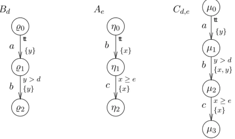
Example 1 Consider the automata Ae, Bd and Cd,e in Figure 1 (d, e ∈ N).
The automatonCd,ehas four nodes, µ0,µ1,µ2and µ3, two clocksxand y, and
three edges. The edge between µ1 and µ2 has b as action, {x, y} as reset set
and the enabling condition for the edge isy > d. 2
3
We extend the transition relation of a timed transition system such thats−→0 s0iffs=s0.
4f(a, b)'cholds iffis defined for the pair (a, b) and the result isc. 5
η2 {x} {y} %2 η1 {x} {y} %1 η0 %0 a b b c µ 2 {x, y} {y} µ1 µ0 a b c {x} µ3 tt tt y > d x≥e tt y > d x≥e Bd Ae Cd,e
Figure 1: Three timed automata
Informally, the system starts at node η0 with all its clocks initialized to
0. The values of the clocks increase synchronously with time. At any time, the automaton whose current node isη can change node by following an edge
hη, η0, a, r, bi ∈E provided the current values of the clocks satisfyb. With this transition the clocks inr get reset to 0.
Formally a time assignment v forC is a function from C toR. We denote by RC the set of time assignments for C. For v ∈ RC, x ∈ C and d ∈ R,
v+d denotes the time assignment which maps each clockx in C to the value
v(x) +d. ForC0 ⊆C, [C07→0]vdenotes the assignment forC which maps each clock in C0 to the value 0 and agrees with v over C\C0. Whenever v ∈ RC,
u∈RK andC and K are disjointvu denotes the time assignment overC∪K
such that (vu)(x) = v(x) if x ∈ C and (vu)(x) = u(x) if x ∈ K. Given a condition b ∈ B(C) and a time assignment v ∈ RC, b(v) is a boolean value describing whether b is satisfied by v or not. Finally a k–clock automata is a timed automatahN, η0, C, Ei such that|C|=k.
A state of an automatonA is a pair (η, v) whereη is a node of A and v a time assignment for C. The initial state of A is (η0, v0) where v0 is the time
assignment mapping all clocks inC to 0.
The semantics of A is given by the timed transition system SA =hSA, σ0, −→Ai, where SA is the set of states of A, σ0 is the initial state (η0, v0), and −→A is the transition relation defined as follows:
(η, v)−→a (η0, v0) iff ∃r, b. hη, η0, a, r, bi ∈E ∧ b(v) ∧ v0 = [r→0]v
(η, v)−→(d)(η0, v0) iff η =η0 and v0 =v+d
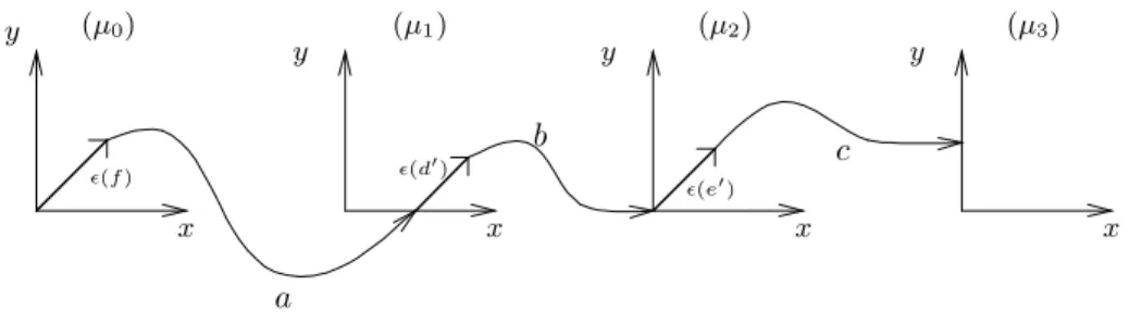
Example 2 Reconsider the automaton Cd,e of Figure 1. The coordinate
sys-tems in Figure 2 indicates (some of) the states of Cd,e. Each point of the
coordinate systems represents a unique time assignment, with the coordinate systems representing states involving the nodesµ0,µ1, andµ2 respectively. We
y x (d0) (µ1) y x (e0) (µ2) y x (µ3) x (f) y (µ0) c b a
Figure 2: Partial Behaviour ofCd,e.
have indicated the following typical transition sequence (where f ≥0, d0 > d
ande0 ≥e): (µ0,(0,0)) (f) −→(µ0,(f, f))−→a (µ1,(f,0)) (d0) −→(µ1,(f +d0, d0)) and (µ1,(f+d0, d0)) b −→(µ2,(0,0)) (e0) −→(µ2,(e0, e0)) c −→ 2
Parallel composition may now be extended to timed automata in the obvious way: for two timed automataA and B and a synchronization function f, the parallel composition A|fB denotes the timed transition system SA|fSb. For
two automata A and B and a synchronization function f one may effectively construct an automatonA⊗fB such thatSA⊗fB is strong bisimilar toSA|f SB.
The nodes of A⊗f B is simply the product of A’s and B’s nodes, the set of
clocks is the (disjoint) union ofA’s and B’s clocks, and the edges are based on synchronizableA and B edges with enabling conditions conjuncted and reset– sets unioned.
Example 3 Let f be the synchronization function completely specified by
f(a,0) = a, f(b, b) = b and f(0, c) = c. Then the automaton Cd,e in
Fig-ure 1 is isomorphic to the part of Bd⊗f Ae which is reachable from (ρ0, η0). 2
3
Timed Logic
We consider a dense–time logic Lν with clocks and recursion. This logic may
be seen as a certain fragment6of theµ–calculus Tµpresented in [HNSY92]. In
[LLW95] it has been shown that this logic is sufficiently expressive that for any timed automaton one may construct a single characteristic formula uniquely characterizing the automaton up to timed bisimilarity. Also, decidability of a satisfiability7 problem is demonstrated.
6
allowing only maximal recursion and using a slightly different notion of model
7
hs, ui |=D tt ⇒ true hs, ui |=Dff ⇒ false hs, ui |=Dϕ∧ψ ⇒ hs, ui |=D ϕ and hs, ui |=Dψ hs, ui |=D∃∃ϕ ⇒ ∃d∈R. hsd, u+di |= Dϕ hs, ui |=D haiϕ ⇒ ∃s0. s−→a s0 and hs0, ui |=D ϕ hs, ui |=D x+m∼y+n ⇒ u(x) +m∼u(y) +n hs, ui |=D xinϕ ⇒ hs, u0i |=D ϕ where u0= [{x} →0]u hs, ui |=D Z ⇒ hs, ui |=D D(Z) Table 1: Definition of satisfiability.
Definition 3 LetKa finite set of clocks,Ida set of identifiers andkan integer. The set Lν of formulae over K, Id and k is generated by the abstract syntax
withϕand ψranging over Lν:
ϕ ::= tt | ff | ϕ∧ψ | ϕ∨ψ | ∃∃ϕ | ∀∀ϕ | haiϕ | [a]ϕ
| xinϕ | x+n∼y+m | Z
wherea ∈ A;x, y ∈ K;n, m ∈ {0,1, . . . , k};∼ ∈ {=, <,≤, >,≥}and Z ∈ Id. The meaning of the identifiers is specified by a declaration D assigning a formula of Lν to each identifier. When D is understood we write Z
def
= ϕ for
D(Z) =ϕ. The K clocks are called formula clocks and a formula ϕ is said to beclosedif every formula clockx occurring inϕis in the scope of an “xin . . .” operator.
Given a timed transition system S we interpret the Lν formulas over an
extended statehs, ui, where sis a state ofS andu is a time assignment forK. Informally,∃∃ϕholds in an extended state if there is a delay transition leading to an extended state satisfying ϕ. Thus ∃∃ denotes existential quantification over (arbitrary) delay transitions. Similarly,∀∀denotes universal quantification over delay transitions, andhai (resp. [a]) denotes existential (resp. universal) quantification over a–transitions. The formula (xinϕ) initializes the formula clock x to 0; i.e. an extended state satisfies the formula in case the modified state with x being reset to 0 satisfies ϕ. Introduced formula clocks are used by formulas of the type (x +n ∼ y+m), which is satisfied by an extended state provided the values of the named formula clocks satisfies the required relationship. Finally, an extended state satisfies an identifier Z if it satisfies the corresponding declaration (or definition) D(Z). Formally, the satisfaction relation |=D between extended states and formulas is defined as the largest relation satisfying the implications of Table 1. We have left out the cases for
∨, [a] and ∀∀as they are immediate duals.
Any relation satisfying the implications in Table 1 is called asatisfiability relation. It follows from standard fixpoint theory [Tar55] that|=D is the union of all satisfiability relations and that the implications in Table 1 in fact are bi– implications for |=D. We say that S satisfies a closed Lν formula ϕand write
S |=ϕwhen hs0, ui |=Dϕ for anyu. Note that ifϕis closed, then hs, ui |=Dϕ
iffhs, u0i |=D ϕfor any u, u0 ∈RK. Similarly, we say that a timed automaton
A satisfies a closed Lν formulaϕ in case SA |=D ϕ. We write A |=D ϕin this
case.
Example 4 Consider the following declarationF of the identifiersXg and Zg
whereg∈N. F = n Xg def= [a] yinZg , Zg def= (y > g)∨ [c]ff∧[a]Zg∧[b]Zg∧ ∀∀Zg o
That isXgexpresses the property that the accumulated time between an initial
a– and a followingc–transition must exceedg. Thus for any transition sequence of the form (whereαi ∈ {a, b}):
s0 a −→t0 (d1) −→s1 α1 −→t2 (d2) −→ s2 α2 −→ · · ·tn (dn) −→sn c −→ P
di > g. Now, reconsider the automata Ae, Bd and Cd,e of Figure 1 and
Ex-amples 1 and 2. Then it may be argued thatCd,e|=F Xd+e and (consequently),
thatBd|f Ae|=F Xd+e. 2
Combining the parameterized parallel composition with Lν we are able to
express timed bisimilarity between timed transition systems as a single for-mula. This provides a timed extension of a similar characterization of strong bisimilarity for finite state systems [And94]: First we close the action set A under tagging; i.e. At= A ∪ A × {l} ∪ A × {r}. Now consider the ‘interleav-ing’ synchronization functionh overAt completely defined byh(a,0) =al and
h(0, a) =ar where a∈ A(i.e. his undefined for all other pairs). Consider the
following declarationE of the identifierZ:
Z def= ^ a∈A [al]hariZ ∧ [ar]haliZ ∧ ∀∀Z
Then timed bisimilarity between timed transition systems is characterized as follows8:
Theorem 1 LetS be a timed transition system overA, and lets1,s2 be states
ofS. Then s1 ∼s2 if and only if s1|hs2 |=E Z.
4
Regions
The model-checking problem for Lν consists in deciding if a given timed
au-tomata A satisfies a given specification ϕ in Lν. In [LLW95] this problem
has been shown decidable using the region technique of Alur and Dill [AD94, ACD90]. The region technique provides an abstract interpretation of timed au-tomata sufficiently complete that all information necessary for model–checking
8It may be shown that the speed relation of [FT91] is characterized in a similar manner by
Y defined recursively byY def= V
with respect to Lν is maintained, yet finitary and thus enabling standard
algo-rithmic model–checking techniques to be applied.
The basic idea is that, given a timed automaton A, two states (η, v1) and
(η, v2) which are close enough with respect to their clocks values (we will say
that v1 and v2 are in the same region) can perform the same actions, and
two extended states h(η, v1), u1i and h(η, v2), u2i where v1 u1 and v2 u2 are
in the same region, satisfy the same Lν formulas 9. The notion of region is
defined as an equivalence class of a relation over time assignments [ACD90]
10 . First, for t ∈ R, let btc def= max{n ∈ N | n ≤ t} denote the integral
part oft, and let {t} def= t− btc denote its fractional part. Moreover we have:
dtedef= min{n∈N | t≤n}.
Definition 4 Let k ∈ N and let C be a set of clocks. Then u, u0 ∈ RC are
equivalent with respect tok, denoted byu=. u0 iff:
i) ∀x∈C. u(x)> k iff u0(x)> k
ii) ∀x∈C s.t. u(x)≤k. bu(x)c=bu0(x)c and {u(x)}= 0 ⇔ {u0(x)}= 0
iii) ∀x, y∈C. u(x)−u(y)> k iff u0(x)−u0(y)> k
iv) ∀x, y∈C s.t. 0≤u(x)−u(y)≤k. bu(x)−u(y)c=bu0(x)−u0(y)c and {u(x)−u(y)}= 0 ⇔ {u0(x)−u0(y)}= 0 The equivalence classes under = are called. regions, and [u] denotes the region which contains the time assignmentu. RC
k denotes the set of all regions
for a setC of clocks and the maximal constantk. From a decision point of view it is important to note thatRCk is finite.
Note that for any condition binB(C) with no constant greater thank, we haveb(u) ⇔ b(u0), whenever u and u0 belong to the same region in RCk. Thus for a regionγ ∈ RCk, we can define b(γ) as the truth value ofb(u) for any uin
γ. Conversely given a region γ, we can easily build a formula of B(C), called
β(γ), such that β(γ)(u) = tt iff u ∈ γ 11. Thus, given a region γ0, β(γ)(γ0) is mapped to the valuettprecisely whenγ =γ0. Finally, note thatβ(γ) itself can be viewed as an Lν formula.
Given a region [u] inRCk andC0 ⊆C we define the following reset operator: [C0 → 0][u] = [[C0 → 0]u]. Moreover, for a region [u], we define the successor region (denoted bysucc([u])) as the region [u0], where:
u0(x) =
u(x) +f ∀x∈C. u(x)> k∨ {u(x)} 6= 0
u(x) +f /2 ∃x∈C. u(x)≤k∧ {u(x)}= 0
wheref =min{1− {u(x)} | u(x)≤k} 12. Informally the change from γ to
succ(γ) correspond to the minimal elapse of time which can modify the enabled actions of the current state.
9
Without loss of generality, we will in all the following assume that that the formula clock setKand the automaton clock set Care disjoint.
10
The notion of region used in the present paper is slightly more refined.
11An obvious way of building β(γ) is to consider the conjunction of all B(C, k) formulas
satisfied by γ, where B(C, k) denotes the finite set (modulo boolean reductions) of B(C) formulas with no constant greater thank.
12
0 (1) (1) 4 5 y x 1 2 3 7 8 9 10 6 14 . . . 0< x <1∧ 0< y <1∧ y=x β(γ0) = (x= 0∧y= 0) 0< x <1∧ 0< y <1∧ succ(γ0) =γ1 succ(γ5) =γ6 β(γ6) = (0< y <1∧x= 1) β(γ1) = β(γ5) = y < x 19 20 21 24 28 18 Figure 3: RC k with C={x, y}and k= 1
We denote byγlthelthsuccessor region ofγ (i.e. γl=succl(γ)). From any regionγ, it is possible to reach a regionγ0 s.t. succ(γ0) =γ0, and we denote by
lγ the required number of steps s.t. γlγ =succ(γlγ).
Example 5 Figure 3 gives an overview of the set of regions defined by two
clocksx and y, and the maximal constant 1. In this case there are 32 different regions, of which only 17 are numbered in the figure. Corresponding B(C)– formulas as well as successor regions are indicated for some of the regions. In general successor regions are determined by following 45o lines upwards to the
right. 2
Given a timed automataA=hN, η0, C, Ei, letkAbe the maximal constant
occurring in the enabling condition of the edges E. Then for any k ≥kA we
can define a symbolic semantics ofA over symbolic states [η, γ]A whereη ∈S
andγ ∈ RCk as follows:
[η, γ]A−→a [η0, γ0]A iff ∃u∈γ, (η, u)−→a (η0, u0) and u0 ∈γ0
[η, γ]A χ
−→[η, succ(γ)]A iff true
Consider now Lν with respect to formula clock setK and maximal constant
kL. Also consider a given timed automata A = hN, η0, C, Ei (s.t. K and C
are disjoint). Then an extended symbolic stateis a pair [η, γ]A+ whereη ∈N
and γ ∈ RCk∪K with k = max(kA, kL). Whenever γ is a region over C ∪K
we denote byγ|C the set of time assignments inγ restricted to the (automata)
clock setC. Similarly,γ|K denotes the projection of all time assignments in γ
to the (formula) clock set K. Observe thatγ|C ∈RC and γ|K∈RK.
Using the finitary symbolic semantics of timed automata a symbolic in-terpretation of Lν is defined in [LLW95] faithfully reflecting the standard
in-terpretation in Table 1. This symbolic inin-terpretation provides the basis for decidability of model–checking for Lν, and consequently (due to Theorem 1)
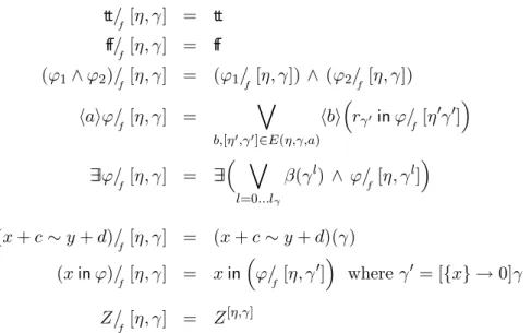
tt/ f [η, γ] = tt ff/f [η, γ] = ff (ϕ1∧ϕ2)/f [η, γ] = (ϕ1/f [η, γ]) ∧ (ϕ2/f[η, γ]) haiϕ/ f [η, γ] = _ b,[η0,γ0]∈E(η,γ,a) hbi rγ0 inϕ/f [η0γ0] ∃∃ϕ/ f [η, γ] = ∃∃ _ l=0...lγ β(γl) ∧ ϕ/ f[η, γ l] (x+c∼y+d)/ f [η, γ] = (x+c∼y+d)(γ) (xinϕ)/ f [η, γ] = xin ϕ/ f[η, γ 0] whereγ0= [{x} →0]γ Z/ f [η, γ] = Z [η,γ]
Table 2: Structural definition of quotient,ϕ/
f[η, γ].
5
Quotienting
Given an Lν formulaϕ, and two timed transition systemsS1 andS2 we aim at
constructing a formula (called thequotient) ϕ/
fS2 such that
S1|fS2 |=ϕ if and only if S1 |=ϕ/f S2 (3)
The bi–implication indicates that we are moving parts of the parallel system into the formula. Clearly, if the quotient is not much larger than the original formula, we have simplified the task of model checking, as the (symbolic) semantics of
S1 is significantly smaller than that ofS1|fS2.
In general it will not be possible to express within Lν such a quotienting
for-mula. However, wheneverS2 is described using a timed automata we are able to express the quotient using the (extended) symbolic semantics of automata. More precisely, whenever ϕ is a formula over K and A is a timed automaton over C, we define quotient formulas ϕ/
f [η, γ] over C ∪K, where [η, γ] is an
extended symbolic state. Forη0 the initial node ofA andγ0 the initial region,
ϕ/
f [η0, γ0] will express the sufficient and necessary requirement to a timed
tran-sition system S in order that S |f SA satisfiesϕ — see also Corollary 3 below.
The quotient construction is defined structurally in Table 2. We have left out the cases for [a], ∨, and ∀∀ as they are immediate duals. The Table uses the following notation: b,[η0γ0]∈ E(η, γ, a) iff [η, γ|C]
c
−→[η0, γ|0C], γ|0K =γ|K and
f(b, c) ' a for some c. We denote by rγ the set of C clocks which has the
value 0 inγ. Moreover (rinϕ) is an abbreviation for (x1in(x2in . . .(xninϕ)))
whenever r is{x1, . . . , xn}. Finally,h0iϕ= [0]ϕ=ϕ.
Note that the quotient construction for identifiers introduces new identifiers of the formZ[η,γ], where Z ∈ Id. The definition of these are collected in the
(quotient) declarationDA given by:
Z[η,γ] def= D(Z)/
f [η, γ]
The following Theorem and Corollary shows that the quotient construction of Table 2 satisfies the requirements of (3). A proof of Theorem 2 is sketched in Appendix A.
Theorem 2 LetS =hS, s0,−→ibe a timed transition system, letA=hN, η0,
C, Ei be a timed automaton, and letϕ be anLν formula over clock set K, all
over an action setA. Then for any s∈S, η∈N,v∈RC, and u∈RK:
D s|f (η, v), u E |=D ϕ if and only if hs, v ui |=DA ϕ/f h η,[v u] i
Corollary 3 LetS be a timed transition system, let Abe a timed automaton
with clock setC, and letϕbe a closedLν formula over clock setK, all over an
action setA. Then:
S |f SA|=D ϕ if and only if S |=DA ϕ/fA where ϕ/
f A abbreviatesϕ/f[η0, γ0] withη0 being the initial node of A and γ0 the initial region overC∪K.
Example 6 Recall the timed automata and declaration from Examples 1 and
4. The quotient X1/f A1 describes the sufficient and necessary requirement to
a timed transition system S in order that S |f SA1 satisfies X1. Clearly, we
expect the timed automata B0 to satisfy this property. Now using a CAML
prototype implementation of the quotient construction X1/f A1 is computed.
The definition ofX1/f A1is found in the quotient declarationFA1 part of which
is given below: X1 fA1 def = [a]yinZ[η0,γ0] 1 Z[η0,γ0] 1 def = ff∨htt∧([b]xinZ[η1,γ0] 1 )∧([a]Z [η0,γ0] 1 )∧ ∀∀ β(γ0) ⇒ Z [η0,γ0] 1 ∧ β(γ1) ⇒ Z [η0,γ1] 1 ∧β(γ2) ⇒ Z [η0,γ2] 1 ∧β(γ3) ⇒ Z [η0,γ3] 1 i Z[η1,γ0] 1 def = ff∨htt∧tt∧([a]Z[η1,γ0] 1 )∧ ∀∀ β(γ0) ⇒ Z [η1,γ0] 1 ∧β(γ1) ⇒ Z [η1,γ1] 1 ∧ β(γ2) ⇒ Z [η1,γ2] 1 ∧β(γ3) ⇒ Z [η1,γ3] 1 i Z[η0,γ1] 1 def = ff∨ h tt∧([b]xinZ[η1,γ18] 1 )∧([a]Z [η0,γ1] 1 )∧ ∀∀ β(γ0) ⇒ Z [η0,γ0] 1 ∧ β(γ1) ⇒ Z [η0,γ1] 1 ∧β(γ2) ⇒ Z [η0,γ2] 1 ∧β(γ3) ⇒ Z [η0,γ3] 1 i Z1[η0,γ2] def= ff∨ h tt∧([b]xinZ1[η1,γ24])∧([a]Z1[η0,γ2])∧ ∀∀ β(γ0) ⇒ Z [η0,γ0] 1 ∧ β(γ1) ⇒ Z [η0,γ1] 1 ∧β(γ2) ⇒ Z [η0,γ2] 1 ∧β(γ3) ⇒ Z [η0,γ3] 1 i Z1[η0,γ3] def= tt∨htt∧([b]xinZ1[η1,γ28])∧([a]Z1[η0,γ3])∧ ∀∀β(γ0) ⇒ Z [η0,γ0] 1 ∧ β(γ1) ⇒ Z [η0,γ1] 1 ∧β(γ2) ⇒ Z [η0,γ2] 1 ∧β(γ3) ⇒ Z [η0,γ3] 1 i
The quotient declaration FA1 contains in total definitions of 96 identifiers.
We expect X1/f A1 to express that the accumulated time between an initial
a–action and a followingb–action must be strictly greater than 0 as described by the following propertyU0:
U0 def = [a] yinV0 V0 def = (y >0)∨ [b]ff∧[a]V0∧ ∀∀V0
In the next section we will present effective minimization strategies, which essen-tially transforms the large quotient declarationFA1 into the small yet equivalent
declaration above. 2
Now, letπ be the synchronization function completely specified byπ(0, a) =
a for all a ∈ A (i.e. the left argument to π is completely ignored). Then it is easy to see that for any timed transition systemS, SA and S |πSA satisfies
the same formulas. In particular SA and S1|πSA satisfies the same formula,
where 1 is the 0–clock timed automaton with just one (initial) node and no edges. Using this observation, the quotient construction can be used to obtain alternative model–checking algorithms for Lν as follows:
Corollary 4 Let A be a timed automaton with clock set C, and let ϕ be a
closedLν formula over clock setK, all over an action set A. Then:
A|=D ϕ if and only if 1 |=DA ϕ/
πA if and only if ϕ/πA⇔tt
Due to the projective nature of π it is clear that ϕ/
πA contains no action
modalities, and it is easy to build a special purpose model checker for the simple automata1.
Example 7 Recall once more the timed automata and declaration from
Ex-amples 1 and 4. From these ExEx-amples we expect thatC0,1satisfies the property
X1. Now, using the Corollary 4 we may verify this by showing that the quotient
formula X1/fC0,1 is either valid or satisfied by 1. X1/fC0,1 is defined in the
following quotient declarationFC0,1
13: X[µ0,γ0] 1 def = xinyinZ[µ1,γ0] 1 Z1[µ1,γ0] def= ∀∀β(γ0) ⇒ Z [µ1,γ0] 1 ∧β(γ1) ⇒ Z [µ1,γ1] 1 ∧β(γ2) ⇒ Z [µ1,γ2] 1 Z1[µ1,γ1] def= (xinZ1[µ2,γ18])∧ ∀∀β(γ0) ⇒ Z1[µ1,γ0]∧β(γ1) ⇒ Z1[µ1,γ1]∧ β(γ2) ⇒ Z1[µ1,γ2] Z[µ2,γ18] 1 def = ∀∀β(γ18) ⇒ Z [µ2,γ18] 1 ∧β(γ19) ⇒ Z [µ2,γ19] 1 ∧β(γ20) ⇒ Z [µ2,γ20] 1 Z1[µ2,γ19] def= ∀∀β(γ18) ⇒ Z1[µ2,γ18]∧β(γ19) ⇒ Z1[µ2,γ19]∧β(γ20) ⇒ Z1[µ2,γ20] Z[µ2,γ20] 1 def = ∀∀ β(γ18) ⇒ Z [µ2,γ18] 1 ∧β(γ19) ⇒ Z [µ2,γ19] 1 ∧β(γ20) ⇒ Z [µ2,γ20] 1 13
Z1[µ1,γ2] def= (xinZ1[µ2,γ24])∧ ∀∀β(γ0) ⇒ Z [µ1,γ0] 1 ∧β(γ1) ⇒ Z [µ1,γ1] 1 ∧ β(γ2) ⇒ Z [µ1,γ2] 1 Z1[µ2,γ24] def= ∀∀β(γ24) ⇒ Z [µ2,γ24] 1 2
Finally, combining the characterization of timed bisimulation in Theorem 1 with the quotient construct of Table 2, we can for any timed automatonA
construct acharacteristicLν formula uniquely characterizing the automaton up
to timed bisimilarity in the following manner: LetE,Z andhbe as in Theorem 1. Then for any timed transition systemS the following holds:
S ∼ SA if and only if S |=E Z/h[η0, γ0]
where η0 is the initial node of A and γ0 is the initial region over the clocks of
A (note that Z is an Lν formula over the empty set of clocks). This provides
an alternative characteristic formula construction compared with [LLW95].
6
Minimizations
It is evident from the examples in the previous section that repeated quotient-ing leads to an explosion in the formula. A similar phenomena was observed by Andersen for the quotient construction of modal µ–calculus formulas with respect to finite–state systems. The crucial observation by Andersen is that simple and cost effective transformations of the formulas in practice often lead to significant reductions.
We have implemented in CAML the quotient construction of the previ-ous section as well as (simplified versions of some of) Andersen’s minimization strategies. In the investigated examples the minimization strategies lead to dra-matic reductions. Below we describe the transformations considered in terms of transformations on formulas and declarations (defining equations).
Reachability: When considering an initial quotient formula ϕ/
f[η0, γ0] not all
identifiers ofDAmay be relevant or reachable. In our CAML implementation an
“on–the–fly” technique insures that only the reachable part ofDAis generated.
Boolean Simplification: Formulas may be simplified using the following simple boolean equations and their duals: ff∧ϕ ≡ ff, tt∧ϕ ≡ ϕ, haiff ≡ ff, ∃∃ff ≡ ff,
xin ff≡ff,haiϕ∧[a]ff≡ff.
Constant Propagation: Identifiers which are declared to either tt or ff may be removed while substituting their definitions in the declaration of all other identifiers.
Trivial Equation Elimination: Equations of the formX def= [a]X are easily seen to haveX=ttas solution. More generally, whenever Xdef= ϕwhereϕ[tt/X]14 can be simplified to tt, we can perform a removal of the identifierX provided the valuett is propagated to all uses ofX (as under Constant Propagation).
Equivalence Reduction: If two identifiers X and Y are equivalent (i.e. are satisfied by the same timed transition systems) we may collapse them into a single identifier. To obtain a cost effective strategy we approximate equivalence of identifiers with the following check: whenever X def= ϕ and Y def= ϑ such thatϕ[Y /X] is syntactically identical toϑ[Y /X] we conclude thatXand Y are equivalent and may be identified.
We apply the above transformation strategies repeatedly on quotient for-mulas and declarations. As can be seen in Table 2, quotienting transforms atomic propositions of the formx+c∼y+d into either tt orff, thus yielding high applicability of Boolean Simplification and Constant Propagation. Also, quotient versions of the same original formula tend to have same structure thus making applicability of Equivalence Reduction high.
In our CAML prototype implementation we have implemented the above re-ported very simple strategies for Trivial Equation Elimination and Equivalence Reduction. Generalized and more sophisticated (yet still efficient) strategies can or course easily be given. However, even with the implemented simple ver-sions we obtain a very high degree of reduction as observed in the following examples.
Example 8 Recall Example 6. Applying the minimization strategies of the
CAML prototype we find thatX1/f A1 is equivalent toY0 with the following
definition: Y0 def = [a]yinY1 Y1 def= [b]ff∧[a]Y1∧ ∀∀ β(γ0) ⇒ Y1∧(β(γ1)∨β(γ2)) ⇒ Y2 Y2 def= [a]Y2∧ ∀∀ β(γ0) ⇒ Y1∧(β(γ1)∨β(γ2)) ⇒ Y2
During minimization only 23 identifiers of FA1 were found to be reachable
from X1/f A1, 14 respectively 3 of which were found to be equivalent to tt
respectivelyff. The remaining 6 identifiers were finally partitioned into 3 classes. Though dramatically reduced, the declaration leaves room for one additional simplification as it may be observed that (β(γ1)∨β(γ2)) ⇒ Y2 is equivalent
tott. With this observation we finally obtain:
Y00 def= [a]yinY10 Y10 def= [b]ff∧[a]Y10∧ ∀∀
β(γ0) ⇒ Y10
which clearly meets the expectations of 6. Minimization of the quotient formula
X7/f A10leads directly to the formulattindicating that for any timed transition
14ϕ[tt/X] is the formula obtained by substituting all occurrences ofX inϕwith the formula
systemS the compositionS |fSA10 satisfiesX7. Intuitively this is clear as the
componentA10 by itself ensures the delay required by X7. The corresponding
quotient declaration contains 3498 identifiers 617 of which were found to be
reachable. Subsequently all these were simplified tott. 2
Example 9 Recall Example 7. Using the minimization strategies of the CAML
prototype we find directly that X1/f C0,1 simplifies to tt thus implying that
C0,1 satisfies the property X1. Similarly, minimization of the quotient formula
X2/f C0,1 yieldsff confirming thatC0,1 does not satisfy X2! 2
Example 10 Now we want to confirm that B0 does indeed satisfy the
re-quirement X1/f A1 and hence that B0|fA1 satisfies X1. Using the equivalent,
minimized formula Y0 from Example 8 it suffices according to Corollary 4 to
verify validity of the quotient formulaY0/πB0. The CAML prototype confirms
this through immediate minimization tott. 2
7
Conclusion
This paper has presented the basis for a compositional model checking technique for real–time systems. Based on initial experiments with the CAML prototype we conjecture that compositional model checking will prove not only a feasible but also an efficient technique for real–time systems. However, it is clear that many more experiments must be performed before the conjecture can be finally settled, and in this process we will need to extend our prototype with more sophisticated minimization strategies as the success of compositional model checking is completely determined by these.
Our work on quotient formulas extends that of [AKLN95], where a quo-tient construction for 1-clock automata has been given. Moreover it can be generalized trivially to logics with minimal fixpoint constructs (such as Tµ in
[HNSY92]) as quotienting is easily seen to distribute over negation.
Acknowledgement
The authors would like to thank Henrik Reif Andersen for interesting and en-lightening discussions on the topic of compositional (partial) model–checking.
References
[ACD90] R. Alur, C. Courcoubetis, and D. Dill. Model–checking for Real–Time Systems. In Proceedings of Logic in Computer Science, pages 414–425. IEEE Computer Society Press, 1990.
[AD94] R. Alur and D. Dill. Automata for Modelling Real–Time Systems. Theo-retical Computer Science, 126(2):183–236, April 1994.
[AKLN95] J. H. Andersen, K. J. Kristoffersen, K. G. Larsen, and J. Niedermann. Automatic Synthesis of Real Time Systems. Lecture Notes in Computer Science, 1995. To appear in Proceedings of ICALP’95.
[And94] H. R. Andersen. A Polyadic Modalµ–calculus. Id–tr: 1994–145, Depart-ment of Computer Science, Technical University of Denmark, 1994. [And95] H. R. Andersen. Partial Model Checking. To appear in Proceedings of
LICS’95, 1995.
[ASW94] H. R. Andersen, C. Stirling, and G. Winskel. A Compositional Proof Sys-tem for the Modal Mu–Calculus. Logic in Computer Science, 1994. [AW92] H.R. Andersen and G. Winskel. Compositional checking of satisfaction.
Formal Methods in Systems Design, 1992. To appear.
[BCM+90] J. R. Burch, E. M. Clarke, K. L. McMillan, D. L. Dill, and L. J. Hwang.
Symbolic Model Checking: 1)20 states and beyond. Logic in Computer
Science, 1990.
[CFJ93] E. M. Clarke, T. Filkorn, and S. Jha. Exploiting Symmetry in Temporal Logic Model Checking. Lecture Notes in Computer Science, 697, 1993. [CGL92] E. M. Clarke, O. Gr¨umberg, and D. E. Long. Model Checking and
Ab-straction. Principles of Programming Languages, 1992.
[EJ93] E. A. Emerson and C. S. Jutla. Symmetry and Model Checking. Lecture Notes in Computer Science, 697, 1993.
[FT91] F.Moller and C. Tofts. Relating Processes with Respect to Speed. Technical Report ECS–LFCS–91–143, Department of Computer Science, University of Edinburgh, 1991.
[GW91] P. Godefroid and P. Wolper. A Partial Approach to Model Checking.Logic in Computer Science, 1991.
[HL89] H. H¨uttel and K. G. Larsen. The use of static constructs in a modal process logic. Lecture Notes in Computer Science, Springer Verlag, 363, 1989. [HNSY92] T. A. Henzinger, Z. Nicollin, J. Sifakis, and S. Yovine. Symbolic model
checking for real-time systems. InLogic in Computer Science, 1992. [Lar86] K.G. Larsen. Context–Dependent Bisimulation Between Processes. PhD
thesis, University of Edinburgh, Mayfield Road, Edinburgh, Scotland, 1986. [LLW95] F. Laroussinie, K. G. Larsen, and C. Weise. From Timed Automata to
Logic — and Back. Technical Report RS–95–2, BRICS, 1995.
[LX90] K.G. Larsen and L. Xinxin. Compositionality through an operational se-mantics of contexts. Lecture Notes in Computer Science, Springer Verlag, 443, 1990. In Proceedings of 17th International Colloquium on Automata, Languages and Programming 1990.
[LX91] K.G. Larsen and L. Xinxin. Compositionality through an operational se-mantics of contexts.Journal of Logic and Computation, 1(6):761–795, 1991. [Mil89] R. Milner. Communication and Concurrency. prentice, Englewood Cliffs,
1989.
[Par81] D. Park. Concurrency and automata on infinite sequences. InProceedings of 5th GI Conference, volume 104 of Lecture Notes in Computer Science, Springer Verlag, Berlin, 1981. Springer.
[Tar55] A. Tarski. A lattice–theoretical fixpoint theorem and its applications. Pa-cific Journal of Math., 5, 1955.
[Val90] A. Valmari. A Stubborn Attack on State Explosion.Theoretical Computer Science, 3, 1990.
[Yi90] W. Yi. A Calculus of Real Time Systems. Lecture Notes in Computer Science, 458, 1990. In Proceedings of CONCUR.
A
Proof of Theorem 2
Proof We only sketch the proof for the identifier free formulas of Lν using
structural induction onϕ. Consequently we drop declaration subscripts on|=. The full proof follows the structure used in [LX90].
We consider only the caseshaiϕ,∃∃ϕand xinϕleaving the remaining more trivial cases to the reader.
• Assume D s|f(η, v), u E |=haiϕ. Then we have: D s|f (η, v), u E |=haiϕ ⇔ Ds0|f(η0, v0), u E
|=ϕ For some s−→a1 s0 and ∃hη, η0, a2, r, bi ∈E
s.t. v0 = [r→0]vand b(v) =ttand f(a1, a2)'a ⇔ hs0, v0ui |=ϕ/ f[η 0,[v0u]] by IH ⇔ hs0, v ui |=rinϕ/ f [η 0,[v0u]] ⇔ hs, v ui |=ha1i(rinϕ/ f[η 0,[v0u]]) ⇔ hs, v ui |= _ a1,[η0,[v0u]]∈E(η,[vu],a) ha1i(rv0inϕ/f [η0,[v0u]]) ⇔ hs, v ui |= (haiϕ)/f h η,[v u] i • Assume D s|f(η, v), u E |=∃∃ϕ. Then we have: D s|f(η, v), u E |=∃∃ϕ ⇔ Dsd|f (η, v+d), u+d E |=ϕ For some d∈R ⇔ hsd, v+d u+di |=ϕ/ f [η,[v+d u+d]] by IH ⇔ hsd, v+d u+di |=ϕ/ f [η,[v u] i] Where (v+d u+d)∈[vu]i ⇔ hsd, v+d u+di |=β([v u]i)∧ϕ/ f [η,[v u] i] ⇔ hs, v ui |= (∃∃ϕ)/ f h η,[v u] i • Assume D s|f(η, v), u E |=xinϕ. Then we have: D s|f(η, v), u E |=xinϕ ⇔ Ds|f(η, v), u0 E |=ϕ with u0= [x→0]u ⇔ hs, v u0,i |=ϕ/ f[η,[v u 0]] by IH ⇔ hs, v ui |=xinϕ/ f [η,[v u 0]] ⇔ hs, v ui |= (xinϕ)/ f h η,[v u] i 2