Statistical Inference in Two-Stage Online Controlled
Experiments with Treatment Selection and Validation
Alex Deng
Microsoft One Microsoft Way Redmond, WA 98052
[email protected]
Tianxi Li
Department of Statistics University of Michigan
Ann Arbor, MI 48109
[email protected]
Yu Guo
Microsoft One Microsoft Way Redmond, WA 98052
[email protected]
ABSTRACT
Online controlled experiments, also called A/B testing, have been established as the mantra for data-driven decision mak-ing in many web-facmak-ing companies. A/B Testmak-ing support decision making by directly comparing two variants at a time. It can be used for comparison between (1) two can-didate treatments and (2) a cancan-didate treatment and an established control. In practice, one typically runs an ex-periment with multiple treatments together with a control to make decision for both purposes simultaneously. This is known to have two issues. First, having multiple treatments increases false positives due to multiple comparison. Second, the selection process causes an upward bias in estimated ef-fect size of the best observed treatment. To overcome these two issues, a two stage process is recommended, in which we select the best treatment from the first screening stage and then run the same experiment with only the selected best treatment and the control in the validation stage. Tra-ditional application of this two-stage design often focus only on results from the second stage. In this paper, we propose a general methodology for combining the first screening stage data together with validation stage data for more sensitive hypothesis testing and more accurate point estimation of the treatment effect. Our method is widely applicable to existing online controlled experimentation systems.
Categories and Subject Descriptors
G.3 [Probability and Statistics]: Experiment Design
General Terms
Measurement, Experimentation, Design, Theory
Keywords
Controlled experiment, A/B testing, Search quality evalua-tion, Meta analysis, Bias correcevalua-tion, Empirical Bayes
Copyright is held by the International World Wide Web Conference Com-mittee (IW3C2). IW3C2 reserves the right to provide a hyperlink to the author’s site if the Material is used in electronic media.
WWW’14,April 7–11, 2014, Seoul, Korea. ACM 978-1-4503-2744-2/14/04.
http://dx.doi.org/10.1145/2566486.2568028.
1.
INTRODUCTION
Controlled experiments have been used in many scientific fields as the gold standard for causal inference, even though only in the recent decade has it been introduced to online services development (Christian 2012; Kohavi et al. 2009; Manzi 2012) where it gained the name A/B testing. At Mi-crosoft Bing, we test everything via controlled experiments, including UX design, backend ranking, site performance and monetization. Hundreds of experiments are running on a daily basis. At any time, a visitor to Bing participates in fifteen or more concurrent experiments, and can be assigned to one of billions of possible treatment combinations (Kohavi et al. 2013).
Surprisingly, the majority of the current A/B testing lit-erature focuses on single stage A/B testing, where one ex-periment (with one or more treatments) is conducted and analyzed at a time. A likely cause could be that A/B test-ing is traditionally conducted at the end of a feature de-velopment cycle, to make final feature ship decision and measure feature impact on key metrics. As A/B testing gains more recognition as one of the most effective sources of data-driven decision making, and with scaling of our ex-perimentation platform, A/B testing is now employed earlier in feature development cycles. Thus comes the need for mul-tiple stages of experiment, in which the results of an earlier screening stage can inform the design of a later validation stage. For example, when there are multiple shipping can-didates, we design the screening stage experiment to select the most promising one. If such a best candidate exists, we conduct a second validation run to make final ship decision and measure treatment effect. This type of two stage exper-iments with treatment selection and validation is commonly used in practice. The space of treatment candidates ranges from 2 to 5 or even 10 in the screening stage. When candi-date number exceeds 10, we can aggressively sift candicandi-dates via offline measurement or “paired test” such as interleaving (Radlinski and Craswell 2013) to boost statistical power in the data analysis.
In this paper, we focus on statistical inference in this two-stage design with treatment selection and validation. The validation stage involves only winner from the screen-ing stage and a control. It is analyzed in the traditional A/B testing framework and is well-understood (Section 2.1). The first screening stage, however, includes simultaneous analy-sis of multiple treatments. We need to adjust hypotheanaly-sis testing procedure to control for inflated false positives in multiple comparison (Section 2.2). We improve on tradi-tional adjustments such as Bonferroni and Holm’s method
(Holm 1979), as they are typically too conservative. In Sec-tion 3 we propose a sharp adjustment method that is exact in the sense that it touches the claimed Type I error. Point estimation is also nontrivial as the treatment selection in-troduces an upward bias (Lemma 4). One might wonder why this is important since in A/B testing people are gen-erally only interested in finding the best candidate to ship. We found in a data driven organization it is equally cru-cial to keep accurate records of impacts made by each in-dividual feature. These records help us understand the re-turn on investment, and prioritize development to benefit users/customers. In Section 4 we propose several methods to correct the bias and investigate more efficient estimators by combining data from both stages. In Section 2.3, we show an insightful theoretical result to ensure we can almost al-ways treat the treatment effect estimates from two stages as independent, given treatment procedures which assign inde-pendently, despite overlap of experiment subjects in the two stages. With this result, we propose our complete recipe of hypothesis testing in Section 3 and several options for point estimation in Section 4.
To the knowledge of the authors, this is the first paper in the context of online controlled experiments that stud-ies the statistical inference for two-stage experiment with treatment selection and validation. This framework can be widely usable in existing online A/B testing systems. Key contributions of our work include:
• A theoretic proof showing negligible correlation
be-tween treatment effect estimates from two stages, given the treatment assignment procedure in the two stages are independent, which is generally useful in theoreti-cal development for all multi-staged experiments.
• A more sensitive hypothesis testing procedure that
correctly adjusts for multiple comparison and utilized data from both stages.
• Several novel bias correction methods to correct the
upward bias from the treatment selection, and their comparison in terms of bias and variance trade-off.
• Demonstration from empirical evidence that we get
more sensitive hypothesis test and more accurate point estimates by combining data from both stages.
2.
BACKGROUND AND WEAK
DEPEND-ENCE BETWEEN ESTIMATES IN TWO
STAGES
Before diving into two-stage model, we first briefly cover the analysis of one stage test. Here we follow the notation in (Deng et al. 2013).
2.1
Treatment vs. Control in One Stage A/B
Test
We focus on the case of the two-sample t-test (Student 1908; Wasserman 2003). Suppose we are interested in a
metric X (e.g. Clicks per user). Assuming the observed
values of the metric for users in the treatment and control
are independent realizations of random variables X(t) for
treatment andX(c) for control respectively, we can apply
the t-test to determine if the difference between the two groups is statistically significant. Under the random user
effect model, for useriin control group,
Xi(c)=µ+αi+ǫi, (1)
whereµis the mean ofX(c),α
irepresents user random effect
and ǫi is random noise. Random user effect αhas mean 0
and variance Var(α). ResidualE[ǫ|α] = 0. The random pair
(αi, ǫi) are i.i.d. for all user. However, we don’t assume
independence of ǫi and αi, as the distribution of ǫ might
depend on α, e.g. users who click more might also have
larger random variation in their clicks. However ǫi andαi
are uncorrelated by construction sinceE(ǫα) =E[E(ǫ|α)] =
0.
For treatment group,
Xi(t)=µ+θi+αi+ǫi,
where fixed treatment effectθcan vary from user to user but
θis uncorrelated to the noiseǫ. The average treatment effect
(ATE) is defined as the expectation ofθ. The null hypothesis
is that δ :=E(θ) = 0 and the alternative is that it is not
0 for a two-sided test. For one-sided test, the alternative
is δ≤0 (looking for positive change) or δ≥0 (looking for
negative change). The t-test is based on the t-statistic:
X(t)−X(c) ò
Var1X(t)−X(c)2
, (2)
where observed difference between treatment and control
∆ = X(t)−X(c) is an unbiased estimator for the shift of
the mean and the t-statistic is a normalized version of that estimator. In traditional t-test (Student 1908), one needs
to assume equal variance and normality ofX(t) and X(c).
In practice, the equal variance assumption can be relaxed by using Welch’s t-test (Welch 1947). For online experi-ments with the sample sizes for both control and treatment at least in the thousands, even the normality assumption on
X is usually unnecessary. To see that, by central limit
the-orem,X(t)andX(c)are both asymptotically normal as the
sample sizemandnfor treatment and control increases. ∆
is therefore approximately normal with variance
Var(∆) = Var1X(t)−X(c)2= Var1X(t)2+ Var1X(c)2.
The statistics (2) is approximately standard normal so t-test in large sample case is equivalent to z-t-test. The central limit theorem only assumes finite variance which almost al-ways applies in online experimentation. The speed of con-vergence to normal can be quantified by using Berry-Essen theorem (DasGupta 2008). We have verified that most met-rics we tested in Bing are well approximated by normal dis-tribution in experiments with thousands of samples.
2.2
Multiple Treatments in A/B Test
When there is only one treatment compared to a cont-rol, ∆ is both the Maximum likelihood estimator (MLE) of the treatment effect, and an unbiased estimator. When
there are multiple treatments and we observe ∆(j) for the
jth treatment, it can be shown that max(∆(j)) is MLE of
max(δ(j)), whereδ(j)is the true underlying treatment effect
of thejth treatment. However, it is obvious that max(∆(j))
is no longer an unbiased estimator. To see this, assuming
δ(j) = 0 for all j, the distributions of ∆(j)’s are
symmet-ric around mean 0. But the distribution of max(∆(j)) will
certainly be skewed to the positive side and with a positive
mean. Note that max(δ(j)) = 0. max(∆(j)) will have a
ifpth treatment is selected (p is random as it is picked as
the best treatment), ∆(p) = max(∆(j)) is not an unbiased
estimator for δ(p).1 Section 4 introduces a novel method
to correct bias so we can achieve a estimator of δ(p) with
smaller mean squared error (MSE).
Besides point estimation, hypothesis testing in experi-ments with multiple treatexperi-ments also suffers from an issue called multiple comparison (Benjamini 2010). Framework of hypothesis testing only guarantees Type I error (False Pos-itive Rate) be controlled under the significant size, which is usually set to 5%, when there is only one test. When there are multiple comparisons, and if we are looking for the “best” treatment among all the treatments, our chance of finding false positive increases. If we have 100 treatments, all have 0 true treatment effect, we still expect to see on
av-erage 5 out of 100 of them showing a p-value below 0.05 just
by chance. To deal with this, various of p-value adjustment techniques have been proposed, such as Bonferroni correc-tion, Holm’s method (Holm 1979) and false discovery rate based methods suitable for even larger number of simulta-neous comparisons (Benjamini and Hochberg 1995; Efron 2010). Both Bonferroni and Holm’s method are applicable to the general case with unknown covariance structure be-tween test statistics of all comparisons. In the context of online A/B testing, when we have large samples, we live in a simpler multivariate normal world. We have full knowl-edge of the covariance structure of this multivariate normal distribution and we should be able to exploit it to come up with a better hypothesis testing procedure. Section 3 contains more details.
2.3
Weak Dependence
When we combine results from two stages to form a more sensitive test and estimate treatment effect more accurately, one of the challenges we face is caused by possible depend-ence of the observed metric values from the two stages. In theory we may force independence between the two stages by running them on separate traffic, so the two stages share no users in in common. This is undesirable in any scaled A/B testing platform (Kohavi et al. 2013) because
1. It means the total traffic in both stages combined can-not exceed 100%, and we suffer from decreased statis-tical power in both stages.
2. It requires additional infrastructure to ensure no over-lap in traffic between the two stages, which can pose technical challenges when we run multiple experiments at the same time.
In this section, we explain why in practice we can safely as-sume independence between the observed ∆ from two stages, as long as the randomization procedure used in the two stages are independent. For online A/B testing, randomiza-tion is usually achieved via bucket assignment. Each ran-domization id, e.g. user id, is transformed into a number
between 0 toK−1 through a hash function and modulo
operation. Independent randomization procedures between any two experiments can be achieved either by using
dif-ferent hashing functions and re-shuffle all K buckets, or
1There is a sutble difference between the two scenarios. In
the former case we use max(∆(j)) to estimate the best
treat-ment effect max(δ(j)) and in the latter case we only want
to estimate the treatment effect of pth treatment without
worrying about whether it is truly the best treatment effect.
preferably, via localized re-randomization described in Ko-havi et al. (2012, Section 3.5).
For the same experiment that has been run twice in the two stages, we model user random effect to be the same for the same user in both stages, but the random noises are independent for different stages. In particular, for a pair of
measurement from the same user (Xi, Yi),
Xi=µ(1)+αi+ǫi, Yi=µ(2)+αi+ζi,
where ǫi and ζi are noise for each run. ǫi and ζi are
in-dependent and all random variables with different index i
are independent. We allow µ(1) to be different from µ(2)
to reflect a change in mean due to some small seasonal ef-fect. After exposure to a treatment, there is an additional
treatment effect termθi in
Xi=µ(1)+θi+αi+ǫi, Yi=µ(2)+θi+αi+ζi,
whereθ is uncorrelated to both noiseǫandζ.
We are now ready for the first result of this paper. Let
N be the total number of users that is available for online
A/B testing. For the screening run, we picked m users as
treatment andnas control. For the second run, we picked
m′ users for treatment and n′ for control. If the random
user picking for the two runs are independent of each other,
let ∆1and ∆2be the observed difference between treatment
and control in the two runs, then
Theorem 1 (Almost Uncorrelated Deltas).
Assuming independent treatment assignment, we have
Cov(∆1,∆2) = Var(θ)/N (3)
Furthermore, if Var(θ)≤ρVar(X) andVar(θ)≤ρVar(Y), then
Corr(∆1,∆2)≤ρ.
This holds whetherm, n, m′, n′ are random variables or
de-terministic.
To understand why Theorem 1 holds, remember N is the
total user size available for experimentation,θ is the
treat-ment effect. Also, Var(∆1) = Var(X(t))/m+ Var(X(c))/n
and similarly Var(∆2) = Var(Y(t))/m′+ Var(Y(c))/n′. We
are interested in the correlation defined by
Corr(∆1,∆2) =
Cov(∆1,∆2)
ð
Var(∆1)×Var(∆2)
=ð Var(θ)/N
Var(∆1)×Var(∆2)
.
If the percentage average treatment effect is d%, then we
argue that Var(θ)/Var(X) is roughly (d%)2. To see this, if
treatment effect is a fixed multiplicative effect, i.e. θ/X =
d%, we have Var(θ) =d%2Var(X). Var(θ)/Var(X) is at the
scale of (d%)2 for any reasonable treatment effect model.
Since N is always larger thanm, n, m′, n′, by (3), we know
Corr(∆1,∆2)≤(d%)2.
In practice, most online A/B testing has a treatment ef-fect less than 10% (In fact a 1% change is quite rare for
many key metrics. If the treatment effect is more than
cheaply gather, detecting such a large effect is usually easy and experimenters don’t need to rely on combining results from multiple stages to increase the power of the test.) This
means Corr(∆1,∆2) ≤0.01 for almost all experiments we
care about in practice, and Corr(∆1,∆2) ≤ 10−4 among
most of the cases.
What does this result entail? Remember in our large
sam-ple setting, ∆1and ∆2 are approximately normal. For
nor-mal distribution, no correlation is equivalent to indepen-dence. The result from the above discussion tells us that in
almost all interesting cases, we can safely treat ∆1 and ∆2
as if they are independent. In two-stage A/B testing with treatment selection and validation, the screening stage in-volves multiple treatments. A straightforward extension of
Theorem 1 shows the vector of observed ∆’s∆1and∆2has
negligible correlation, hence are almost independent. Fur-thermore, for hypothesis testing purpose (Section 3), un-der null hypothesis, we assume there is no treatment effect. Hence we know correlation between ∆ from two stages would
be less than (d%)2, thanks to Theorem 1, which is 0.
We make our final remark to close this section. In the
model we assumed the user effectαand the treatment effect
θ for two runs of the same experiment to be the same for
the same user. This can also be relaxed to allow both user effect and treatment effect for the same user in two runs to be a bivariate pair with arbitrary covariance structure.
Theorem 1 still holds if we change Var(θ) in (3) to covariance
of the treatment effect.
3.
HYPOTHESIS TESTING
In statistics, combining results from different studies is the subject of a field called meta-analysis. In this section we present a method for hypothesis testing utilizing data from both stages. Using combined data for point estimation is discussed in Section 4.
3.1
Meta-Analysis: Combine Data from Two
Stages
Suppose we conduct two independent hypothesis tests and
observed two p-valuesp1andp2. A straightforward attempt
of combing two “probability of falsely rejecting null hypoth-esis” would be to multiply the two p-values together, and
claim the productp=p1×p2 to be the p-value of the
com-bined test. This seemingly sound approach actually pro-duce p-values smaller than the true Type I error. To see
this, under null hypothesis, p-values p1 and p2 follow the
uniform(0,1) distribution. Type I error of combined test is
P(U1×U2≤p) whereU1 andU2 are two independent
uni-form(0,1) distributed random variables. This probability can be calculated using a double integral:
Ú
xy≤p,0≤x,y≤1
dxdy=p(1−logp). (4)
Sincep <1, Type I errorp(1−logp)> p. The
underesti-mation of Type I error could be very significant for common
p-values. Whenp=p1×p2 = 0.1, the true Type I error if
we reject the null hypothesis would be 3.3×0.1, meaning the
true Type I error is underestimated by more than 3 times if we simply multiply the two p-values.
Equation (4) provides the correct p-value calculation the-oretically. To use it in hypothesis testing for usual p-value
cutoff at 0.05, the productprequired to makep(1−logp)≤
0.05 is 0.0087.
The calculation of true Type I error when multiplying more than 2 p-values quickly becomes cumbersome. Fisher (Fisher et al. 1970) noticed natural log function transforms uniform(0,1) distribution into an exponential(1) distribution
and exponential(1) is half of aχ2with 2 degrees of freedom.
In this connection, the product ofkp-values under null
hy-pothesis is sum of independent exponential(1) and
2 log(Ùpi) =
Ø
(2 log(pi))∼χ22k.
This result, known as the Fisher’s method, can be used to combine tests under the assumption of independent p-values. It is also a model-free method in the sense that it only utilizes p-value without tapping into the distribution of test statistics. It is not surprising that in our cases, by using normality and known covariance structure of our observed ∆’s, we should be able to get a more sensitive test. We leave this extension in Section 3.2.
However, we still have the multiple comparison issue to tackle. One standard method is Bonferroni correction. Spe-cifically,
1. First we determine the p-value from the screening stage
using a Bonferronni correction. If there isKtreatment
candidates in the screening run, ifp1 the smallest
p-value, we just divide this p-value byK.
2. We use this value plus the p-value for the second stage and combine using Fisher’s method.
This combined with Fisher’s method provides a valid hy-pothesis testing for two-stage A/B testing with treatment selection and validation. We will just call it BF method and set it as our benchmark.
3.2
Sharp Multiple Comparison Adjustment
In this section we improve BF method in two directions. We will use a sharper multiple comparison adjustment. We also exploit known distribution properties to form a test statistic. We call our method generalized weighed average method since the test statistic is in a form of weighted av-erage.
Although Bonferroni correction is the simplest and most widely used multiple comparison adjustment, it is often too conservative in online controlled experiments. This is be-cause by central limit theorem, we can safely assume all metrics to be approximately normal. More specifically, let
X1, X2, . . . , Xk be the observed metric values (e.g. clicks
per user) for the k treatments and X0 be the value for the
control, we can estimate the variance of each and take these as known in our model. Moreover, the covariance between ∆i, i = 1, . . . , k can also be estimated. In this scenario
of complete distributional information, we can use a gen-eralized step-down procedure (Romano 2005, Section 9.1, p.352).
Generalized step-down procedure
Given observed ∆1, . . . ,∆k, we first test against the null
hy-pothesis that all treatments are no greater than 0. In the screening stage we assign equal traffic size for all treatments.
We use max(∆i) as the test statistics. ∆1, . . . ,∆k follows
a multivariate normal distribution with known covariance matrix. We can theoretically compute the distribution of
max(∆i) under the least favorable null hypothesis, which is
when all treatment effects are 0 (Toothaker 1993, Appendix 3, p.374). In practice, we resort to Monte Carlo
simula-tion. We simulateBi.i.d random samples from multivariate
normal distribution with mean 0 and the estimated
covari-ance matrix. For each trial we record the max(∆i). The
simulated B data points serve as an empirical null
distri-bution of max(∆i). A p-value can then be calculated using
the empirical distribution. The step-down procedure rejects the null hypothesis for the treatment with the largest ∆. Then it take the remaining ∆’s and continue the same test against the null hypothesis for this subset of treatments. This procedure stops when the test fails to reject the subset null hypothesis and it accepts them all. It can be proved that this procedure, like Bonferroni correction, controls the family-wise false positive rate. But it is strictly less conser-vative than Bonferroni correction. A two-sided test would
be looking at the extreme value, i.e. max(abs(∆i)) with
otherwise the same procedure.
For our purpose of testing two-stage experiments with treatment selection and validation, we can stop at the first step, since we only care about the selected treatment with the largest ∆ at the screening stage. How do we combine this with the validation stage ∆? If there are no multiple treatments at the screening stage, we are just replicating the same experiment twice. Thanks to Theorem 1, we can treat the two ∆’s as independent. Then any weighted average of the two would be an unbiased estimator for the underlying treatment effect. We define
∆c=w∆(1)+ (1−w)∆(2),
where ∆(1)and ∆(2)stands for the observed ∆ in two stages
respectively. To minimize the variance of this unbiased
es-timator, the optimal weight w would be proportional to
1/Var(∆(s)), s= 1,2. This combined test statistics is also
normally distributed, and therefore can be standardized into a Z-score. We call it combined Z-score method.
Generalized weighted average test
To adopt combined Z-score test to support treatment se-lection in the screening stage, we modify the test statistics as:
∆c=wmax(∆i) + (1−w)∆∗,
where ∆∗is the observed ∆ at the validation stage for the
selected treatment form the screening stage. The optimal
weight can also be estimated, by calculating Var(max(∆i))
theoretically or from simulation. We then form empirical null distribution through simulation with this test statistic, and calculate p-values. This method is in spirit the same as the combined Z-score, just with an adjustment to the null distribution.
This generalized weighted average test is more favorable comparing to more generic methods such as BF method. It exploits the know distributional information otherwise ig-nored. It is sharp in the sense that it would touch the desig-nated Type I error bound, unlike BF method. The reason is, it does not rely on loose probability inequalities such as Bon-ferroni inequality, which was required to control for Type I error for all forms of tests. Instead it relies on simulation to get the exact Type I error, no more, no less. The weighted average method combines the data from two stages nicely and optimally. We compare generalized weighted average
test to BF method in Section 5.1. The same idea of using weighted average will also be used in Section 4 for point estimation of the treatment effect.
4.
POINT ESTIMATION
Another task for A/B testing is to provide good estimation of the true treatment effects, in terms of minimal mean-squared error (MSE) that achieves a balance between bias and variance.
In the screening stage of the experiment, suppose we have
kdifferent treatments with metric valuesX1, . . . , Xk
respec-tively. Thanks to the central limit theorem, we can assume
X= (X1, X2, . . . , Xk)T∼ N(µ,Σ) whereµ= (µ1, . . . , µk)T
and Σ = diag(σ2
1, . . . , σk2)2. Moreover, there is a control
group with the metric value X0 ∼ N(µ0, σ02). The
esti-mation of σi is easy to achieve with a large sample and
of no interest in this paper, thus we assume the variances are known and fixed. Without loss of generality, assume
σ = σ0 = · · · = σk. Then we can use ∆i = Xi−X0 as
the estimation of the effect of the ith treatment. At the
end of the screening stage, we choose the treatment with
the largest ∆ by maxi = argmaxi∆i = argmaxiXi, then
run the second-stage experiment with only the control group
and themaxith treatment.
In the validation stage, Xmaxi∗ ∼ N(µmaxi, σ′2) for the
selected treatment is obtained, as well as the new
obser-vation for control group X∗
0 ∼ N(µ0, σ′2). Let ∆∗maxi =
Xmaxi∗ −X0∗. According to Theorem 1, we can ignore the
dependence between the observed ∆’s from the two stages.
To estimate the true treatment effect δ = µmaxi−µ0,
∆∗maxiis the MLE and also is unbiased thus optimal for the
validation stage. However, according to Lemma 4, ∆maxi
is actually upward biased. Thus a traditional choice for
the point estimation is only by ∆∗maxi. The MSE for this
estimator isσ2. It is clear that this method is less efficient
as we ignore the useful information from the screening stage.
Denote ˜∆maxias the estimation in the screening stage. For
weighted average ˆδw=w·δˆmaxi+ (1−w)·∆∗maxi:
MSE(ˆδw) =w2MSE(ˆδmaxi) + (1−w)2σ′2. (5)
The bestwthat minimizes the MSE can be found by solving
w
(1−w) =
σ′2
MSE( ˜∆maxi). In practice, even by a naive choice
of w = 1/2, we are guaranteed to have a better MSE if
MSE(ˆδmaxi)<3σ2. Thus the task in this section is to find
a good estimator ˆδmaxi for the screening stage, or
equiva-lently, a good estimator ˆµmaxiforµmaxi, as we can always let
ˆ
δmaxi = ˆµmaxi−X0. X0 is independent of Xi, i= 1, . . . , k
and does not suffer from the selection bias, and it is also
optimal forµ0.
Let ˆµmaxi,M LE be the estimator for Xmaxi. Define the
bias of MLE asλ(µ) =Eµ(Xmaxi−µmaxi). λ(µ) is positive
as shown in Lemma 4. So we seek a bias correction forλ(µ),
and propose the following estimators:
2Usually the metric X is in a form of average. We useX
here to simplify the notation. Metric can also be a ratio of averages, such as Clicks Per Query. For this kind of met-ric, vector of numerator and denominator follows a bivariate normal distribution under central limit theorem with known covariance structure. We can then use the delta method to calculate variance of the metric.
Naive-correction estimator
Based on the screening stage observationX =x, simulate
Bindependentyb∼N(x, σ2I). Calculate the expected bias
λ from the simulated samples. Then use ˆµmaxi,naive =
Xmaxi−λˆ as the estimator. Note that this is actually a
“plug-in" estimation as ˆλ(µ) =λ(x). Denote this estimator
as ˆµmaxi,naive.
Compared to ˆµmaxi,M LE, the naive-correction has smaller
bias but larger variance.
Var(ˆµmaxi,naive)
= Var(ˆµmaxi,M LE) + Var(λ(X))−2Cov(ˆµmaxi,M LE, λ(X))
in which Cov(ˆµmaxi,M LE, λ(X)) can be expected to be
neg-ative. This makes ˆµmaxi,naive inferior when the true
esti-mation bias of ˆµmaxi,M LEis small, as can be seen from
sim-ulation results in Section 5.2. The slight bias in the naive-correction is immaterial for the performance according to our evaluation.
Inspired by the drawback of the naive-correction, we seek some simpler factor that could account for the major factor but with a smaller variance. Apparently the gap between the
largestµi and the second largestµi can be a major factor
for the bias. However,µis unknown so an alternative with
similar information is needed. AssumeX(1), X(2)...X(k) are
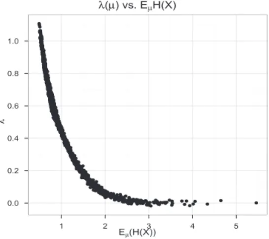
the order statistics. Define the first order gap asH(X) =
X(k)−X(k−1) √
2σ2 , then biasλ(µ) is roughly monotonic with the
average observed H(X). Thus H can be seen as a major
factor for the bias in the sense of expectation. Such rela-tionship can be observed in Figure 1, which is produced
by 2000 randomly sampledµ’s as described in Section 5.2.
Similarly, one can define higher order gap such as theith
or-der gap asHi(X) =
X(k)−X(k−i) √
2σ2 and try to fitλ(µ) beyond
univariate function.
λ(µ) vs. EµH(X)
Eµ(H(X))
λ 0.0 0.2 0.4 0.6 0.8 1.0 ● ● ● ● ● ● ● ● ● ● ● ● ● ● ● ● ● ● ● ● ● ● ● ● ● ● ● ● ● ● ● ● ● ● ● ● ● ● ● ● ● ● ● ● ● ● ● ● ● ● ● ● ● ● ● ● ● ● ● ● ● ● ● ● ● ● ● ● ● ● ● ● ● ● ● ● ● ● ● ● ● ● ● ● ● ● ● ● ● ● ● ● ● ● ● ● ● ● ● ● ● ● ● ● ● ● ● ● ● ● ● ● ● ● ● ● ● ● ● ● ● ● ● ● ● ● ● ● ● ● ● ● ● ● ● ● ● ● ● ● ● ● ● ● ● ● ● ● ● ● ● ● ● ● ● ● ● ●● ● ● ● ● ● ● ● ● ● ● ● ● ● ● ● ● ● ● ● ● ● ● ● ● ● ● ● ● ● ● ● ● ● ●● ● ● ● ● ● ● ● ● ● ● ● ● ● ● ● ● ● ● ● ● ● ● ● ● ● ● ● ● ● ● ● ● ● ● ● ● ● ● ● ● ● ● ● ● ● ● ● ● ● ● ● ● ● ● ● ● ● ● ● ● ● ● ● ● ● ● ● ● ● ● ● ● ● ●● ● ● ● ● ● ● ● ● ● ● ● ● ● ● ● ● ● ● ● ● ● ● ● ● ● ● ● ● ● ● ● ● ● ● ● ● ● ● ● ● ● ● ● ● ● ● ● ● ● ● ● ● ● ● ● ● ● ● ● ● ● ● ● ● ● ● ● ● ● ● ● ● ● ● ● ● ● ● ● ● ● ● ● ● ● ● ● ● ● ● ● ● ● ● ● ● ● ● ● ● ● ● ● ● ● ● ● ● ● ● ● ● ● ● ● ● ● ● ● ● ● ● ● ● ● ● ● ● ● ● ● ● ● ● ● ● ● ● ● ● ● ● ● ● ● ● ● ● ● ● ● ● ● ● ● ● ● ● ● ● ● ● ● ● ● ● ● ● ● ● ● ● ● ● ● ● ● ● ● ● ● ● ● ● ● ● ● ● ● ● ● ● ● ● ● ● ● ● ● ● ● ● ● ● ●● ● ● ● ● ● ● ● ● ● ● ● ● ● ● ● ● ● ● ● ● ● ● ● ● ● ● ● ● ● ● ● ● ● ● ● ● ● ● ● ● ● ● ● ● ● ● ● ● ● ● ● ● ● ● ● ● ● ● ● ● ● ● ● ● ● ● ● ● ● ● ● ● ● ● ● ● ● ● ● ● ● ● ● ● ● ● ● ● ● ● ● ● ● ● ● ● ● ● ● ● ● ● ● ● ● ● ● ● ● ● ● ● ● ● ● ● ● ● ● ● ● ● ● ● ● ● ● ● ● ● ●● ●● ● ● ● ● ● ● ● ● ● ● ● ● ● ● ● ● ● ● ● ● ●● ● ● ● ● ● ● ● ● ● ● ● ● ● ● ● ● ● ● ● ● ● ● ● ● ● ● ● ● ● ● ● ● ● ● ● ● ● ● ● ● ● ● ● ● ● ● ● ● ● ● ● ● ● ● ● ● ● ● ● ● ● ● ● ● ● ● ●● ● ● ● ● ● ● ● ● ● ● ● ● ● ● ● ● ● ● ● ●● ● ● ● ● ● ● ● ● ● ● ● ● ● ● ● ● ● ● ● ● ● ● ● ● ● ● ● ● ● ● ● ● ● ● ● ● ● ● ● ● ● ● ● ● ● ● ● ● ● ● ● ● ● ● ● ● ● ● ● ● ● ● ● ● ● ● ● ● ● ● ● ● ● ● ● ● ● ● ● ● ● ● ● ● ● ● ● ● ● ● ● ● ● ● ● ● ● ● ● ● ● ● ● ● ● ● ● ● ● ● ● ● ● ● ● ● ● ● ● ● ● ● ● ● ● ●● ● ● ● ● ● ● ● ● ● ● ● ● ● ● ● ● ● ● ● ● ● ● ● ● ● ● ● ● ● ● ● ● ● ● ● ● ● ● ● ● ● ● ● ● ● ● ● ● ● ● ● ● ● ● ● ● ● ● ● ● ● ● ● ● ● ● ● ●● ● ● ● ● ● ● ● ● ● ● ● ● ● ● ● ● ● ● ● ● ● ● ● ● ● ● ● ● ● ● ● ● ● ● ● ● ● ● ● ● ● ● ● ● ● ● ● ● ● ● ● ● ● ● ● ● ● ● ● ● ● ● ● ● ● ● ● ● ● ● ● ● ● ● ● ● ● ● ● ● ● ● ● ● ● ● ● ● ● ● ● ● ● ● ● ● ● ● ● ● ● ● ● ● ● ● ● ● ● ● ● ● ● ● ● ● ● ● ● ● ● ● ● ● ● ● ● ● ● ● ● ● ● ● ● ● ● ● ● ● ● ● ● ● ● ● ● ● ● ● ● ● ● ● ● ● ● ● ● ● ● ● ● ● ● ● ● ● ● ● ● ●● ● ● ● ● ● ● ● ● ● ● ● ● ● ● ● ● ● ● ● ● ● ● ● ● ● ● ● ● ● ● ● ● ● ● ● ● ● ● ● ● ● ● ● ● ● ● ● ● ● ● ● ● ● ● ● ● ● ● ● ● ● ● ● ● ● ● ● ● ● ● ● ● ● ● ● ● ● ● ● ● ● ● ● ● ● ● ● ● ● ● ● ● ● ● ● ● ● ●● ● ● ● ● ●● ● ● ● ● ● ● ● ● ● ● ● ● ● ● ● ● ● ● ● ● ● ● ● ● ● ● ● ● ● ● ● ● ● ● ● ● ● ● ● ● ● ● ● ● ● ● ● ● ● ● ● ● ● ● ● ● ● ● ● ● ● ● ● ● ● ● ● ● ● ● ● ● ● ● ● ● ● ● ● ● ● ● ● ● ● ● ● ● ● ● ● ● ● ● ● ● ● ● ● ● ● ● ● ● ● ● ● ● ● ● ● ● ● ● ● ● ● ● ● ● ● ● ● ● ● ● ● ● ● ● ● ● ● ● ● ● ● ● ● ● ● ● ● ● ● ● ● ● ● ● ● ● ● ● ● ● ● ● ● ● ● ● ● ● ● ● ● ● ● ● ● ● ● ● ● ● ● ● ● ● ● ● ● ● ● ● ● ● ● ● ● ● ● ● ● ● ● ● ● ● ● ● ● ● ● ● ● ● ● ● ● ●● ● ● ● ● ● ● ● ● ● ● ● ● ● ● ● ● ● ● ● ● ● ● ● ● ●● ● ● ● ● ● ● ● ● ● ● ● ● ● ● ● ● ● ● ● ● ● ● ● ● ● ● ● ● ● ● ● ● ● ● ● ● ●● ● ● ● ● ● ● ● ● ● ● ● ● ● ● ● ● ● ● ● ● ● ● ● ● ● ● ● ● ● ● ● ● ● ● ● ● ● ● ● ● ● ● ● ● ● ● ● ● ● ● ● ● ● ● ● ● ● ● ● ● ● ● ● ● ● ● ● ● ●● ● ● ● ● ● ● ● ● ● ● ● ● ● ● ● ● ● ● ● ● ● ● ● ● ● ●● ● ● ● ● ● ● ● ● ● ● ● ● ● ● ● ● ● ● ● ● ● ● ● ● ● ● ● ● ● ● ● ● ● ● ● ● ● ● ● ● ● ● ● ● ● ● ● ● ● ● ● ● ● ● ● ● ● ● ● ● ● ● ● ● ● ● ● ● ● ● ● ● ● ● ● ● ● ● ● ● ● ● ● ● ● ● ● ● ● ● ● ● ● ● ● ● ● ● ● ● ● ● ● ● ● ● ● ● ● ● ● ● ● ● ● ● ● ● ● ● ● ● ● ● ● ● ● ● ● ● ● ● ● ● ● ● ● ● ● ● ● ● ● ● ● ● ● ● ● ● ● ● ● ● ● ● ● ● ● ● ● ● ● ● ● ● ● ● ● ● ● ● ● ● ● ● ● ● ● ● ● ● ● ● ● ● ● ● ● ● ● ● ● ● ● ● ● ● ● ● ●●● ● ● ● ● ● ● ● ● ● ● ● ● ● ● ● ● ● ● ● ● ● ● ● ● ● ● ● ● ● ● ● ● ● ● ● ● ● ● ● ● ● ● ● ● ● ● ● ● ● ● ● ● ● ● ● ● ● ● ● ● ● ● ● ● ● ● ● ● ● ● ● ● ● ● ● ● ● ● ● ● ● ● ● ● ● ● ● ● ● ● ● ● ● ● ● ● ● ● ● ● ● ● ● ● ● ● ● ● ● ● ● ● ● ● ● ● ● ● ● ● ● ● ● ● ● ● ● ● ● ● ● ● ● ● ● ● ● ● ● ● ● ● ● ● ● ● ● ● ● ● ● ● ● ● ● ● ● ● ● ● ● ● ● ● ● ● ● ● ● ● ● ● ● ● ● ● ● ● ● ● ● ● ● ● ● ● ● ● ● ● ● ● ● ● ● ● ● ● ● ● ● ● ● ● ● ● ● ● ● ● ● ● ● ● ● ● ● ● ● ● ● ● ● ● ● ● ● ● ●
1 2 3 4 5
Figure 1: Theλ(µ) =Eµ(xmaxi−µmaxi) and Eµ(H(x)) of 2000 randomly sampledµ’s.
Simple linear-correction estimator
Based on observationX=x, simulateB independentyb∼
N(x, σ2I), b = 1· · ·B. For each yb, denote the gap
be-tween max(yb) and the correspondingxcovariate asd(yb) =
max(yb)−xargmax(yb) andH(yb). Model the relation
d(y)∼f(H(y)) (6)
by linear models. We recommend using natural cubic splines (cubic splines with linear constraints outside boundary knots)
for the model. Take the expected bias ˆλas the model
pre-diction on H(x) and use ˆµmaxi = xmaxi−ˆλ+ as the
esti-mation. Call this NSestimation. Simulation shows that its
performance is robust against the choice of the exact linear form. For instance, using cubic polynomial regression would achieve similar performance according to our evaluation.
The intuition behind the simulation inNSis that suppose we
can can simulate fromN(µ, σ2I), then we should be able to
have a very good recovery ofλ∼f(H(µ)). However since
we don’t knowµ, we need a reasonable population is by
gen-erating random samples in a similar way as how we getX.
InNS, we use a “plug-in" population to simulate the data we
need.
Bayesian posterior driven linear-correction esti-mator
Since the naive correction based on MLE suffers from high variance, we try Bayesian approach to avoid over-fitting the
data for a low variance estimator. Assume a prior µ ∼
N(0, τ2I)3. Here we take an empirical Bayes approach to
construct the posterior mean and variance as shown in (Efron and Morris 1973) — the posterior mean turns out to be the famous James-Stein estimator (Stein 1956; James and Stein 1961). Then the formula becomes
µ|X∼ N((1−(k−2)σ
2
ëXë2 2
)X,(1−(k−2)σ
2
ëXë2 2
)σ2I).
When the shrinkage (1− (kë−X2)ë2σ2
2
) ≤0, we take it as zero
and it becomes a posterior asP(µ= 0) = 1. We call the
posterior constructed in this way JS posterior. This gives
another estimator: forb= 1, . . . , B, we first sampleµbfrom
theJSposterior, and then sampleyb∼ N(µb, σ2I). All the
remaining modeling steps are the same as NS. We call this
JS-NS estimation. Intuitively, compared to NS,JS-NS uses hierarchical sampling based on a shrinkage estimation by us-ing an empirical Bayesian prior which is expected to make the model fitting more robust, thus giving a lower variance. Nevertheless, since the posterior shrinks the estimation
to-ward 0, JS-NS estimate the bias well when true treatment
effects are close to 0 but can over-correct the bias when bias
is small. We seeJS-NSas a further step beyoundNSto lower
variance by allowing for some remaining biases. See Efron (2011) for another application of Empirical Bayes based se-lection bias correction.
Beyond simple linear-correction
One can further explore more sophisticated (multivariate and non-linear) modeling under the logic of linear-correction. A few examples are included for completeness in Section 5.2. However, we observe no significant gains.
We can set a large number B of simulation trials to fit
the functional form (6), as the computation is simple and
fast. We observed that beyond B >10000, more runs no
longer make much difference. For the natural cubic splines,
3It is also possible to assume a general prior mean, which
will shrink the estimation to the mean ofXinstead. Such
estimation will consume one more degree of freedom and
result in factor k-3 instead of k-2 in shrinkage. However,
in most applications of online experiments, X has limited
dimension thus one might prefer to save that one degree of freedom.
one can simply choose the simple version by using 3 knots.
It turns out that theNSestimator with this setting achieved
the best compromise between the bias and variance out of the candidates, which will be illustrated in more details in the Section 5.2. In practice, when using weighted average to combine this estimator with the second validation stage MLE, we don’t know the MSE of the estimator and therefore can not get the optimal weight. However, it is reasonable to use weights inverse proportional to the sample size in formula (5), i.e. assume MSE of the two estimators in two stages are the same for the same sample size.
5.
EMPIRICAL RESULTS
5.1
Empirical Results for Hypothesis Testing
In this section we use simulation to compare the BF method to the generalized weighed average method. To simulate the two-stage controlled experiments with treatment selection and validation, we assume a pair of measurement from the same user comes from a bivariate normal distribution with
pairwise correlation coefficientρ= 0.5 between stages, and
variance 1. The choice of the variance 1 here is irrelevant because one can always scale a distribution to unit variance. The correlation coefficient here is also less important. Also note that the specific distribution of this user level mea-surement is not very important because of the central limit theorem. For treatment effect, we set a treatment effect on
each user using a normal distributionN(θ, σ2θ).
For each run of experiment, we randomly generatedN =
1000 pairs of such samples from the bi-variate normal distri-bution, representing 1000 users entering into the two stages of the experiment. In each run we randomly assign equal proportions to be treatments and control respectively. In
the screening stage, there arek = 4 treatment candidates
and we select the best one to run the validation stage. In
the context of Theorem 1, this means m =n =N/5 and
m′=n′=N/2. The random sampling for the two runs are
independent.
Type I error under the null hypothesis
We study Type I error achieved by BF method and general-ized weighted average method under the least favorable null where all treatment effects are 0. We seek positive treatment effects as our alternative hypothesis. For two stage exper-iments, when validation run shows a ∆ that is in different direction comparing to the screening stage run, it generally means the findings in the screening stage cannot be repli-cated and it then make less sense trying to combine the two
runs. Therefore, when either of the two ˆδwere negative, we
set pvalues to 1.
We ran 10,000 simulation trials to show Type I error
un-der null hypothesis where all treatment effects are 0. It con-firms our claim that BF method is too conservative, with a
3.2% true Type I error. On the other hand, our generalized
weighted average approach (WAvg), at 5.1% closely touches
the 5% Type I error as promised.
We then assess the impact of the small correlation in The-orem 1 that was ignored when we performed the test. Al-though under the least favorable null hypothesis, treatment effects are all 0 and the correlation is exactly 0, we can still relax the null hypothesis and add some variance in the
random user treatment effect θ. To do that, we assume
even though E(θ) = 0, but Var(θ) = 0.04. Since we set
the variance of user level measurement to be 1, this setting means the random treatment effect has a standard deviation of 20% of that of the user level measurement. As we dis-cussed, a 10% treatment effect is already already very rare for online A/B testing, needless to mention 20%. To test the robustness of the test against the impact of the correlation
between the two stages, we ran another 10,000 trials when
treatment effect has a 20% standard deviation and observe
the same phenomenon. BF method has a 3.3% true Type I
error while WAvg still achieves 5.0%.We see that both
gen-eralized weighted average and BF method are very robust. This empirically justifies Theorem 1 that we can safely ig-nore the small correlation between the two stages. How-ever, Theorem 1 also shows as the variance of user random
treatment effect Var(θ) gets larger, the correlation could be
significant. As an extreme case, we did the same simulation
for Var(θ) = 1, i.e., treatment random effect has the same
standard deviation as the measurement itself. We found the Type I error of generalized weighted average method
in-creased to 12.3% while for BF method it stayed at 4.2%.
This suggests BF method might be more robust against the correlation than generalized weighted average method.
Statistical power under the alternative hypothesis
Next we compare the sensitivity of the two tests under
al-ternative. We increaseN to 110,000 and let the treatment
effect vary from 0 to 0.03 with step size 0.001. We also
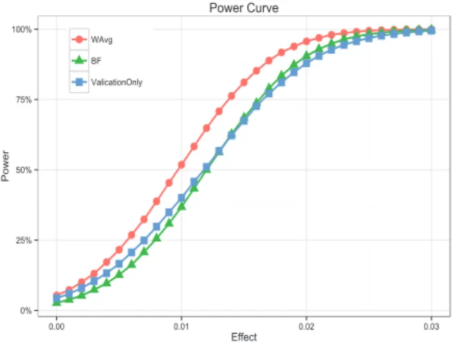
in-creased the number of treatments to 10 and set the same treatment effect on them. Figure 2 shows the power curve estimated from 10000 simulation runs. We observed that BF method could be inferior to validation run t-test for small treatment effects, even though it tried to take advantage of data from the screening run. By contrast, generalized weighted average method had higher power than both of them for the whole range, with a gap of 10% to 15% for the
middle range. Whenµ= 0.015, power for weighted average
method was 81% and the power for BF and validation run t-test was only at around 68%. Hence we’ve seen generalized weighted average method is more sensitive.
!
Figure 2: Power curve of generalized weigthed aver-age method, BF method and validation run t-test.
To evaluate the proposed estimators of µmaxi, we
sim-ulated 200 experiments with four treatments each, their
meansµ fromN(η,4I), whereη= (2,2,2,2)T is irrelevant
to the estimation. Without loss of generality, we useσ= 1
in simulation. Then for each experiment, we generated 1500
independent random vectorsxwith meanµ, and calculated
their MSE Note we can only observe onexin practice. In
all the estimations, theB is chosen to be 10000. The knots
for splines were chosen as the (0.1,0.5, 0.9) quantiles of the
simulatedH(yb).
Three additional methods were included for completeness: the bi-variate natural splines estimation and boosted trees
with two variables for bias correction viaH(X) andH2(X).
The bi-variate splines model is an example of including more predictors: setting the basis functions with 6 degree of free-dom for both of the two variates without any interaction
term. We label this estimatorNS-2and the corresponding
univariate version asNS-1. The boosted trees can be seen as
an example when one seeks to model the bias exhaustively by using the two predictors (but still in a regularized way). In each estimation of equation 6, all base trees were required to be of depth 3 (so at most 2 orders of interaction will be considered in each base learner), and 1200 trees were trained in each estimation, with final prediction model selected ac-cording to hold-out squared prediction error. We label this
estimator as Boost. The last estimator is a mixture
be-tween MLE andJS-NSaccording to the rule: ifH(X)>1
take MLE as the estimator and otherwise use JS-NS. The
intuition behind this will be explained in Remark 1. We
label it asMLE-JSNS-Mixture. Many threshold values other
than 1 were evaluated as well but they all suffer from the same problem which will be discussed later.
In addition to MSE, the bias and variance of each es-timators were also studied respectively. For the clearness
of illustration, only 16µ’s are shown in detail below, with
error bars for the MSE and biases estimated by 1500
in-stantiations. These 16µ are representative for the general
case according to our observations. The error bars of the variance are too small to be shown, thus were ignored. The
16 µ’s are ordered according to the first order gap H(µ).
In each figure, they are also split into two groups: the ones
withH(µ)>1 and those withH(µ)<1.
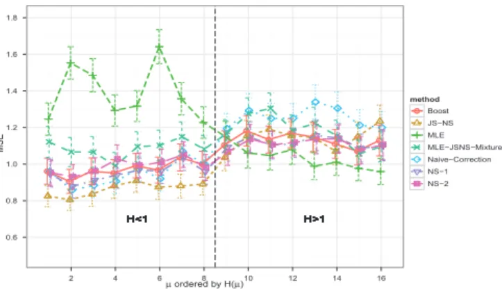
Figure 3 shows that MLE has smaller bias and larger
vari-ance when H(µ) is large and vice versa. When the true
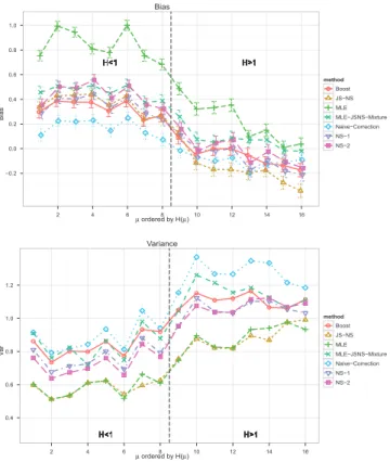
bias is small, the naive correction become inferior to MLE while in other cases, it achieves much smaller MSE. Fig-ure 4 shows that naive-correction results in minimum bias on average, but has large variance. Thus it will be outper-formed by MLE when the gain in bias is small. On the
other hand,NS-1achieved a good compromise between the
two. It performs nearly as good as naive-correction when naive-correction works well, while still retains reasonably
good MSE when the naive-correction fails. Neither NS-2
norBoost seems to improve the performance. Thus using the univariate linear estimator is the best choice among the
candidates.JS-NSperforms significantly better than others
in the case of H(µ) < 1, and closely toNS for moderate
H(µ). Figure 4 reveals the advantage of JS-NS. The
vari-ance of JS-NS is always similar to MLE, much lower than
all other variables. This means using hierarchical sampling with JS posterior does help to make the estimation stable.
As discussed before,JStends to over-correct the bias when
H(µ) is large though as shown in the bias plot. In summary,
JS-NSis the best one in most cases whileNSis a good choice if one conservatively prefers a good performance uniformly.
Remark 1. Figure 3 indicates a simple rule of selecting correction method: ifH(µ)is large, use MLE, otherwise use correction estimation (for instance, JS-NS). Since µ is un-known in practice, one alternative is to use observed H(X)
instead. This is the intuition for MLE-JSNS-Mixture and
its variants. However, it turns out that these estimators perform poorly in many cases due to the large variances as shown in Figure 4, though the biases are small. Using
H(X) > 1 introduces extra variance that degraded perfor-mance of the estimators.
Remark 2. When H(µ) is large, all candidates except MLE have higher MSE than σ2. Such extra MSE is the
price we have to pay for not knowing the oracle of whether we need bias correction beforehand. In the best cases, the MSE of the final estimation is lower than σ2, even better
than the case of single random variable. This is an effect of “learning from the experience of others" discussed in Efron (2010). That is, sinceµi’s are close in such cases, knowing
allxi’s could help to improve the estimation.
µ ordered by H(µ)
MSE
0.6 0.8 1.0 1.2 1.4 1.6 1.8
H<1 H<1 H<1 H<1 H<1 H<1 H<1 H<1 H<1 H<1 H<1 H<1 H<1 H<1 H<1 H<1 H<1 H<1 H<1 H<1 H<1 H<1 H<1 H<1 H<1 H<1 H<1 H<1 H<1 H<1 H<1 H<1 H<1 H<1 H<1 H<1 H<1 H<1 H<1 H<1 H<1 H<1 H<1 H<1 H<1 H<1 H<1 H<1 H<1 H<1 H<1 H<1 H<1 H<1 H<1 H<1 H<1 H<1 H<1 H<1 H<1 H<1 H<1 H<1 H<1 H<1 H<1 H<1 H<1 H<1 H<1 H<1 H<1 H<1 H<1 H<1 H<1 H<1 H<1 H<1 H<1 H<1 H<1 H<1 H<1 H<1 H<1 H<1 H<1 H<1 H<1 H<1 H<1 H<1 H<1 H<1 H<1 H<1 H<1 H<1 H<1 H<1 H<1 H<1 H<1 H<1 H<1 H<1 H<1 H<1 H<1
H<1 H>1H>1H>1H>1H>1H>1H>1H>1H>1H>1H>1H>1H>1H>1H>1H>1H>1H>1H>1H>1H>1H>1H>1H>1H>1H>1H>1H>1H>1H>1H>1H>1H>1H>1H>1H>1H>1H>1H>1H>1H>1H>1H>1H>1H>1H>1H>1H>1H>1H>1H>1H>1H>1H>1H>1H>1H>1H>1H>1H>1H>1H>1H>1H>1H>1H>1H>1H>1H>1H>1H>1H>1H>1H>1H>1H>1H>1H>1H>1H>1H>1H>1H>1H>1H>1H>1H>1H>1H>1H>1H>1H>1H>1H>1H>1H>1H>1H>1H>1H>1H>1H>1H>1H>1H>1H>1H>1H>1H>1H>1H>1H>1
2 4 6 8 10 12 14 16
method
Boost
JS−NS MLE MLE−JSNS−Mixture Naive−Correction NS−1 NS−2
Figure 3: The estimated MSE for candidate estima-tors on 16 of the 200 randomly generated µ’s. The µ’s are ordered according the value H(µ) and are grouped byH(µ)<1 andH(µ)>1.
6.
CONCLUSION
When data-driven decision making via online controlled experiment becomes a culture and the scale of an online A/B testing platform reaches a point when anyone can and should run their ideas through A/B testing, it is almost cer-tain that A/B testing will eventually be employed through the full cycle of web-facing software developments. This is already happening now at Microsoft Bing. In this paper, we took our first steps to build the theoretical foundation for one of the multi-stage designs that is already a common practice — two-stage A/B testing with treatment selection and validation.
The results and methods we laid out in this paper are more general even though motivated primarily by this spe-cific design. Using generalized step-down test to adjust for multiple comparison can be applied to any A/B testing with relatively few treatments. Bias correction methods are use-ful when one cares about a point estimate and our empirical
Bias
µ ordered by H(µ)
Bias
−0.2 0.0 0.2 0.4 0.6 0.8 1.0
H<1 H<1 H<1 H<1 H<1 H<1 H<1 H<1 H<1 H<1 H<1 H<1 H<1 H<1 H<1 H<1 H<1 H<1 H<1 H<1 H<1 H<1 H<1 H<1 H<1 H<1 H<1 H<1 H<1 H<1 H<1 H<1 H<1 H<1 H<1 H<1 H<1 H<1 H<1 H<1 H<1 H<1 H<1 H<1 H<1 H<1 H<1 H<1 H<1 H<1 H<1 H<1 H<1 H<1 H<1 H<1 H<1 H<1 H<1 H<1 H<1 H<1 H<1 H<1 H<1 H<1 H<1 H<1 H<1 H<1 H<1 H<1 H<1 H<1 H<1 H<1 H<1 H<1 H<1 H<1 H<1 H<1 H<1 H<1 H<1 H<1 H<1 H<1 H<1 H<1 H<1 H<1 H<1 H<1 H<1 H<1 H<1 H<1 H<1 H<1 H<1 H<1 H<1 H<1 H<1 H<1 H<1 H<1 H<1 H<1 H<1
H<1 H>1H>1H>1H>1H>1H>1H>1H>1H>1H>1H>1H>1H>1H>1H>1H>1H>1H>1H>1H>1H>1H>1H>1H>1H>1H>1H>1H>1H>1H>1H>1H>1H>1H>1H>1H>1H>1H>1H>1H>1H>1H>1H>1H>1H>1H>1H>1H>1H>1H>1H>1H>1H>1H>1H>1H>1H>1H>1H>1H>1H>1H>1H>1H>1H>1H>1H>1H>1H>1H>1H>1H>1H>1H>1H>1H>1H>1H>1H>1H>1H>1H>1H>1H>1H>1H>1H>1H>1H>1H>1H>1H>1H>1H>1H>1H>1H>1H>1H>1H>1H>1H>1H>1H>1H>1H>1H>1H>1H>1H>1H>1H>1
2 4 6 8 10 12 14 16
method Boost JS−NS MLE MLE−JSNS−Mixture Naive−Correction NS−1 NS−2
Variance
µ ordered by H(µ)
V
ar
0.4 0.6 0.8 1.0 1.2
H<1 H<1 H<1 H<1 H<1 H<1 H<1 H<1 H<1 H<1 H<1 H<1 H<1 H<1 H<1 H<1 H<1 H<1 H<1 H<1 H<1 H<1 H<1 H<1 H<1 H<1 H<1 H<1 H<1 H<1 H<1 H<1 H<1 H<1 H<1 H<1 H<1 H<1 H<1 H<1 H<1 H<1 H<1 H<1 H<1 H<1 H<1 H<1 H<1 H<1 H<1 H<1 H<1 H<1 H<1 H<1 H<1 H<1 H<1 H<1 H<1 H<1 H<1 H<1 H<1 H<1 H<1 H<1 H<1 H<1 H<1 H<1 H<1 H<1 H<1 H<1 H<1 H<1 H<1 H<1 H<1 H<1 H<1 H<1 H<1 H<1 H<1 H<1 H<1 H<1 H<1 H<1 H<1 H<1 H<1 H<1 H<1 H<1 H<1 H<1 H<1 H<1 H<1 H<1 H<1 H<1 H<1 H<1 H<1 H<1 H<1
H<1 H>1H>1H>1H>1H>1H>1H>1H>1H>1H>1H>1H>1H>1H>1H>1H>1H>1H>1H>1H>1H>1H>1H>1H>1H>1H>1H>1H>1H>1H>1H>1H>1H>1H>1H>1H>1H>1H>1H>1H>1H>1H>1H>1H>1H>1H>1H>1H>1H>1H>1H>1H>1H>1H>1H>1H>1H>1H>1H>1H>1H>1H>1H>1H>1H>1H>1H>1H>1H>1H>1H>1H>1H>1H>1H>1H>1H>1H>1H>1H>1H>1H>1H>1H>1H>1H>1H>1H>1H>1H>1H>1H>1H>1H>1H>1H>1H>1H>1H>1H>1H>1H>1H>1H>1H>1H>1H>1H>1H>1H>1H>1H>1
2 4 6 8 10 12 14 16
method Boost JS−NS MLE MLE−JSNS−Mixture Naive−Correction NS−1 NS−2
Figure 4: The estimated biases and variances for candidate estimators on the 16µ’s. The µ’s are or-dered according the valueH(µ) and are grouped by H(µ)<1and H(µ)>1.
results shed lights on how to find further correction methods with even smaller MSE The theoretical proof of weak corre-lation between estimators from multiple stages is a general result that is applicable beyond two stages.
We wish to point out one concern here. In our model we did not consider any carryover effect. In multi-stage experi-ments when there is overlap of subjects (traffic) at different stages, treatment effect from first exposure may linger even after the treatment is removed. To eliminate carryover ef-fect, one can use separate traffic for different stages. In practice, however, we didn’t find evidence of strong carry-over effect in most of the experiments we run or if any, such effects usually fade away after a few weeks’ wash-out period. However, we have observed cases where carryover effect can linger for weeks or even months, such as examples we shared in (Kohavi et al. 2012, Section 3.5). One proposed solution is to segment users in the validation stage by their treatment assignment in the screening stage. This is equivalent to in-cluding another categorical predictor in the random effect model. If there is no statistically significant benefit from introducing this additional predictor, we assume there is no carryover effect from Occam’s razor principle.
7.
ACKNOWLEDGMENTS
We wish to thank Brian Frasca, Ron Kohavi, Paul Raff and Toby Walker and many members of the Bing Data Min-ing team. We also thank the anonymous reviewers for their valuable feedback.
References
Yoav Benjamini. Simultaneous and selective inference:
cur-rent successes and future challenges.Biometrical Journal,
52(6):708–721, 2010.
Yoav Benjamini and Yosef Hochberg. Controlling the false discovery rate: a practical and powerful approach to
mul-tiple testing. Journal of the Royal Statistical Society.
Se-ries B (Methodological), pages 289–300, 1995.
Brian Christian. The a/b test: Inside the technology that’s
changing the rules of business, April 2012. URL http:
//www.wired.com/business/2012/04/ff_abtesting/.
Anirban DasGupta. Asymptotic Theory of Statistics and
Probability. Springer, 2008.
Alex Deng, Ya Xu, Ron Kohavi, and Toby Walker. Im-proving the sensitivity of online controlled experiments
by utilizing pre-experiment data. In Proceedings of the
sixth ACM international conference on Web search and data mining, pages 123–132. ACM, 2013.
Bradley Efron.Large-scale inference: empirical Bayes
meth-ods for estimation, testing, and prediction, volume 1. Cambridge University Press, 2010.
Bradley Efron. Tweedie’s formula and selection bias.Journal
of the American Statistical Association, 106(496):1602– 1614, 2011.
Bradley Efron and Carl Morris. Stein’s estimation rule and
its competitors–an empirical bayes approach. Journal
of the American Statistical Association, 68(341):117–130, 1973. ISSN 01621459.
Sir Ronald Aylmer Fisher, Statistiker Genetiker,
Ronald Aylmer Fisher, Statistician Genetician, Great Britain, Ronald Aylmer Fisher, and Statisticien
Généti-cien.Statistical methods for research workers, volume 14.
Oliver and Boyd Edinburgh, 1970.
Sture Holm. A simple sequentially rejective multiple test
procedure. Scandinavian journal of statistics, pages 65–
70, 1979.
W. James and James Stein. Estimation with quadratic loss.
In Jerzy Neyman, editor,Proceedings of the Third
Berke-ley Symposium on Mathematical Statistics and
Probabil-ity, pages 361–379. University of California Press, 1961.
Ron Kohavi, Roger Longbotham, Dan Sommerfield, and Randal M. Henne. Controlled experiments on the web:
survey and practical guide. Data Mining Knowledge
Dis-covery, 18:140–181, 2009.
Ron Kohavi, Alex Deng, Brian Frasca, Roger Longbotham, Toby Walker, and Ya Xu. Trustworthy online controlled
experiments: Five puzzling outcomes explained.
Proceed-ings of the 18th Conference on Knowledge Discovery and Data Mining, 2012.
Ron Kohavi, Alex Deng, Brian Frasca, Toby Walker nd Ya Xu, and Nils Pohlmann. Online controlled
experi-ments at large scale. Proceedings of the 19th Conference
on Knowledge Discovery and Data Mining, 2013.
Jim Manzi. Uncontrolled: The Surprising Payoff of
Trial-and-Error for Business, Politics, and Society. Basic Books, 2012.
Filip Radlinski and Nick Craswell. Optimized interleaving
for online retrieval evaluation. InProceedings of the sixth
ACM international conference on Web search and data mining, pages 245–254. ACM, 2013.