ISSN: 2252-8938, DOI: 10.11591/ijai.v8.i4.pp399-410 399
Improving software development effort estimation using
support vector regression and feature selection
Abdelali Zakrani1, Mustapha Hain2, Ali Idri31,2Department of Industrial Engineering, ENSAM, Hassan II University, Morocco 3Software Project Management Research Team, ENSIAS, Mohammed V University, Morocco
Article Info ABSTRACT
Article history: Received Aug 15, 2019 Revised Oct 30, 2019 Accepted Nov 15, 2019
Accurate and reliable software development effort estimation (SDEE) is one of the main concerns for project managers. Planning and scheduling a software project using an inaccurate estimate may cause severe risks to the software project under development such as delayed delivery, poor quality software, missing features. Therefore, an accurate prediction of the software effort plays an important role in the minimization of these risks that can lead to the project failure. Nowadays, the application of artificial intelligence techniques has grown dramatically for predicting software effort. The researchers found that these techniques are suitable tools for accurate prediction. In this study, an improved model is designed for estimating software effort using support vector regression (SVR) and two feature selection (FS) methods. Prior to building model step, a preprocessing stage is performed by random forest or Boruta feature selection methods to remove unimportant features. Next, the SVR model is tuned by a grid search approach. The performance of the models is then evaluated over eight well-known datasets through 30%holdout validation method. To show the impact of feature selection on the accuracy of SVR models, the proposed model was compared with SVR model without feature selection. The results indicated that SVR with feature selection outperforms SVR without FS in terms of the three accuracy measures used in this empirical study.
Keywords:
Accuracy measures Random forest
Software effort estimation Support vector regression feature selection
Copyright © 2019 Institute of Advanced Engineering and Science. All rights reserved.
Corresponding Author: Abdelali Zakrani,
Department of Industrial Engineering, Ecole Nationale Supérieure d’Arts et Métiers,
150 Avenue Nile, Sidi Othman, 20670, Casablanca, Morocco. Email: [email protected]
1. INTRODUCTION
In an age of regular technological disruption, for software companies, growing fast has become essential to survival. Moreover, software companies must also target becoming profitable rapidly and efficiently. One of the main keys to achieve this goal is to allocate software project resources efficiently and schedule activities as optimally as possible. In this context, estimating software development effort is critical. Various methods have been investigated in software effort estimation, including traditional methods such as the constructive cost model (COCOMO) [1], and, recently, machine learning techniques such as MLP neural networks [2], radial basis function (RBF) neural networks [3], random forest (RF) [4-5] , fuzzy analogy (FA) [6] and support vector regression (SVR) [7]. Machine learning techniques use data from past projects to build a regression model that is subsequently employed to predict the effort of new software projects. However, no single method has been found to be entirely stable and reliable for all cases. Furthermore, the performance of any method depends mainly on the characteristics of the dataset used to construct the model. These characteristics include dataset size, outliers, number of features, categorical features and missing values. Therefore, performing a preprocessing data prior to any SDEE model building can contribute to improve the
accuracy of the generated estimation. Depending on dataset used, the preprocessing data can be cleaning data by imputing missing value or transforming and/or reducing the data by removing redundant and irrelevant features. As one of the major concerns when using dataset to construct a SDEE model is the negative impact of irrelevant and redundant information on estimation accuracy [8].
Hence, we need to remove irrelevant and redundant information and keep a subset of relevant features so only information about the effort (dependent variable) is reserved. For this purpose, many feature selection (FS) methods have been employed in the literature [8-13]. In this context, this paper aims to investigate the use of two feature selection methods as preprocessing step before feeding data to SVR model building stage. The paper aims also to evaluate whether or not the wrapper feature selection methods improve the accuracy of the SVR model. Therefore, we assess SVR models preprocessed with two wrapper methods and we compare them with SVR model built without feature selection methods. The main contributions of this paper are threefold: (1) assessing the impact of feature selection methods on the predictive capability of SVR models over eight datasets (2) employing two wrapper feature selection methods to select the attributes used for SVR models (3) tuning the hyperparameter values of SVR using a grid search approach and 10-fold cross-validation approach. This paper is organized as follows. Section 2 presents the SVR technique and the two feature selection methods used in this study and Section 3 gives an overview of related work conducted on SVR in SDEE. In Section 4, we describe the architecture of the proposed model including the methodology adopted to adjust it parameters values. Section 5 presents a brief description of the datasets, the accuracy measures, the validation method used in this study. The empirical results are presented and discussed in Section 6. Finally, Section 7 concludes the paper.
2. BACKGROUND
Before entering into details, we introduce the three main tools of this paper: support vector regression, feature importance, and feature selection.
2.1. Support vector regression
Support Vector Machines as described in [14] have shown to deliver promising solutions in various classification and regression tasks thanks to their ability to avoid local minima, improved generalization capability, and sparse representation of the solution. SVM are based on Structural Risk Minimization (SRM) principle and thus tries to control the upper bound of generalization risk while reducing the model complexity. In addition, they do not suffer from over fitting problem and local minimization issues and hence offer enhanced generalization capability. For regression tasks, Vapnik proposed an SVM called ε-support vector regression (ε-SVR), which performs prediction tasks from the ε-insensitive loss function. Because the ε parameter is useful if the approximation accuracy is specified beforehand, it is better to find a procedure to optimize this accuracy without depending a priori on a value set. This procedure was studied by Sölkopf, Smola, Williamson and Bartlett [15]. They proposed a new formulation, called ʋ-support vector regression (ʋ-SVR), that automatically minimizes the ε-insensitive loss function and changes the SVR formulation by using a new ʋ parameter whose value is between [0,1]. In addition to minimizing the ε value, the ʋ parameter is used for controlling the number of support vectors, since the value of ε influences the choice of support vectors.
In this study, a special form of SVM i.e., Support Vector Regression (SVR) is utilized for modeling the input–output functional relationship or regression purpose and is explained next. Given a set of input– output sample pairs {(𝑥1, 𝑦1), (𝑥2, 𝑦2), . . . , (𝑥𝑛, 𝑦𝑛)} where 𝑥𝑖 ∈ 𝐼𝑅𝑝and 𝑦𝑖∈ 𝐼𝑅, the objective of ν-SVR
technique is to approximate the nonlinear relationship given in (1), such that 𝑓(𝑥) should be as close as possible to the target value y and should be as flat as possible in order to avoid over-fitting.
𝑓(𝑥) = 𝑤𝑇. 𝜑(𝑥) + 𝑏 (1)
where 𝑤𝑇 is the weight vector, 𝑏 is the bias and 𝜑(𝑥) represents the transformation function that maps the
lower dimensional input space to a higher dimensional space. The primal objective of the problem thus reduces to (2), in order to ensure that the approximated function meets the above two objectives of closeness and flatness.
minimize 1
2‖𝑤‖
2+ 𝐶 {𝛾. 𝜀 +1
2∑ (𝜉 + 𝜉
∗) 𝑛
subject to the
constraints {
𝑦𝑖− 〈𝑤𝑇. 𝜑(𝑥)〉 − 𝑏 ≤ 𝜀 + 𝜉𝑖∗,
〈𝑤𝑇. 𝜑(𝑥)〉 + 𝑏 − 𝑦
𝑖≤ 𝜀 + 𝜉𝑖∗,
𝜉𝑖, 𝜉𝑖∗≥ 0
where ε is a deviation of a function f(x) from its actual value and, ξ, ξi*are additional slack variables introduced by Cortes & Vapnik, 1995, which determines that, deviations of magnitude ξ above ε error are tolerated. The constant C known as regularization parameter determines the tradeoff between the flatness of f and tolerance of error above ε. Further ϒ (0≤ϒ≤1), represents the upper bound on the function of margin errors in the training set and establishes the lower bound on the fraction of support vectors. To solve the primal problem in (2), its dual formulation is introduced by constructing Lagrange function (L) given as:
𝐿: 1
2‖𝑤‖
2+ 𝐶 {Υ. 𝜀 +1
𝑛∑ (𝜉 + 𝜉
∗) 𝑛
𝑖=1 } −
1
𝑛∑ (𝜂. 𝜉 + 𝜂
∗𝜉∗) 𝑛
𝑖=1 −
1
𝑛∑ (𝜀 + 𝜉1− 𝑤
𝑇. 𝜑(𝑥) − 𝑏) 𝑛
𝑖=1 +
1
𝑛∑ (𝜀 + 𝜉𝑖− 𝑤
𝑇. 𝜑(𝑥) + 𝑏) − 𝛽. 𝜀 𝑛
𝑖=1 (3)
where 𝛼, 𝛼∗, 𝜂, 𝜂∗ 𝑎𝑛𝑑 𝛽 are Lagrange multipliers and 𝛼(∗)= 𝛼. 𝛼∗. Thus, maximizing the Lagrange function
gives 𝑤 = ∑𝑛𝑖=1(𝛼𝑖− 𝛼𝑖∗). 𝜑(𝑥𝑖) and yields the following dual optimization problem:
maximizes
−1
2∑ (𝛼𝑖− 𝛼𝑖
∗). (𝛼 𝑗− 𝛼𝑗∗) 𝑛
𝑖,𝑗=1
. 𝐾(𝑥𝑖, 𝑥𝑗) + ∑ 𝑦𝑖. (𝛼𝑖− 𝛼𝑖∗); 𝑛
𝑖=1
subject to {
∑𝑛𝑖=1(𝛼𝑖− 𝛼𝑖∗) = 0,
∑𝑛𝑖=1(𝛼𝑖− 𝛼𝑖∗) ≤ 𝐶𝛶,
𝛼𝑖, 𝛼𝑖∗∈ [0, 𝐶 𝑛]
(4)
where 𝐾(𝑥𝑖, 𝑥𝑗) denotes the kernel function given by 𝐾(𝑥𝑖, 𝑥𝑗) = 𝜑(𝑥𝑖)𝑇. 𝜑(𝑥𝑗). The solution to (4) yields
the Lagrange multipliers 𝛼, 𝛼∗. Substituting weight w in (1), the approximated function is given as:
𝑓(𝑥) = ∑𝑛𝑖=1(𝛼𝑖− 𝛼𝑖∗).𝐾(𝑥𝑖, 𝑥) + 𝑏 (5)
The choice of kernel function for specific data patterns, which is another attractive question in the application of SVR, appeared somewhat arbitrary till now. Some previous work [6, 16] empirically indicate that the use of the gaussian RBF kernel is superior to other kernel functions because of its accessibility to implement and powerful mapping capability. Therefore, the gaussian RBF kernel function, (6), was employed in this study.
𝐾(𝑥𝑖, 𝑥𝑗) = exp (−𝛾‖𝑥𝑖− 𝑥𝑗‖ 2
) 𝑤ℎ𝑒𝑟𝑒 𝛾 = 1
2𝜎2 (6)
The parameter σ affects the mapping transformation of the input data to the feature space and controls the complexity of the model, thus, and the value of parameter 𝛾 should be selected carefully and adequately. In addition, SVR requires also setting two parameters: the complexity parameter usually denoted by C, the extent to which deviations (i.e., errors) are tolerated denoted by Epsilon (ε), and the ʋ parameter which is used for controlling the number of support vectors, since the value of ε influences the choice of support vectors.
2.2. Feature selection methods
This subsection provides an overview of the feature selection methods with particular focus on feature importance concept used by the methods used in this paper.
2.2.1. Feature selection methods
Feature selection, also known as variable selection, is the process of identifying the most promising features (variables, attributes) in a given dataset. The selected feature will be used to construct the model or as inputs of a prediction system. There are many potential benefits of feature selection such as improving the generalization performance of the predictive model, reducing the computational time to construct the model,
and better understanding the underlying process. Several feature selection methods have been proposed and studied in the literature [17]. They can fall into three categories: the wrapper, the filter and embedded. The wrapper methods use a predictive model to score feature subsets. Each new subset is used to train a model, which is tested on a hold-out set. Counting the number of mistakes made on that hold-out set (the error rate of the model) gives the score for that subset [18]. The filter methods consider statistical characteristics of a data set directly without involving any learning algorithm. The embedded methods combine feature selection and the learning process in order to select an optimal subset of features. In general, the results of wrapper methods are better than those of filter methods. However, the wrapper method is slow (time-consuming) and very complicated when there are many features in the dataset. Fortunately, in our case, the datasets used in this study have relatively a small number of features.
2.2.2. Random forest feature importance
Random forest (RF) is an ensemble learning technique based on classification and regression trees [19]. Each tree is trained on a bootstrap sample, and optimal variables at each split are identified from a random subset of all variables. The selecting criteria are different for classification and regression problems. For the former setting, the Gini index is applied, whereas variance reduction is used for the latter approach. The global prediction of the RF is computed as a majority vote or average for classification or regression, respectively [20]. In addition to prediction, RFs can be used as method to estimate variable importance measures to rank variables by predictive importance. To illustrate this, let’s 𝐹𝑗 a
project feature. RF feature importance of 𝐹𝑗is defined, as described in [21], as follows. For each tree t of the
forest, consider the associated 𝑂𝑂𝐵𝑡 sample (Out Of Bag is the data which was not included in the boostrap
sample used to construct 𝑡). Denote by 𝑒𝑟𝑟𝑂𝑂𝐵𝑡 the mean square error (MSE) of a single tree t on this 𝑂𝑂𝐵𝑡
sample. Now, randomly permute the values of 𝐹𝑗 in 𝑂𝑂𝐵𝑡to get a perturbed sample denoted by 𝑂𝑂𝐵𝑡 𝑗
̌ and
compute 𝑒𝑟𝑟𝑂𝑂𝐵𝑡𝑗, the error of predictor t on the perturbed sample. Feature importance of 𝐹𝑗is then equal to:
𝐹𝑒𝑎𝑡𝐼𝑚𝑝(𝐹𝑗) =
1
𝑛𝑡𝑟𝑒𝑒∑ (𝑡 𝑂𝑂𝐵𝑡 𝑗
̌ − 𝑒𝑟𝑟𝑂𝑂𝐵𝑡
𝑗
), (7)
where the sum is over all trees 𝑡of the RF and 𝑛𝑡𝑟𝑒𝑒 denotes the number of trees of the RF. Features that are relevant for prediction will have large importance values, whereas features that are not associated with the outcome have values close to zero.
2.2.3. Boruta feature selection method
Boruta is an all relevant feature selection algorithm, i.e., embedded with the RF algorithm and uses calculated Z-scores as a measure of band importance. The main idea of this approach is to compare the importance of the real predictor variables with those of random so-called shadow variables using statistical testing and several runs of RFs [22]. In each run, the set of predictor variables is doubled by adding a copy of each variable. The values of those shadow variables are generated by permuting the original values across observations and therefore destroying the relationship with the outcome. A RF is trained on the extended data set and the variable importance values are collected. For each real variable a statistical test is performed comparing its importance with the maximum value of all the shadow variables. Variables with significantly larger or smaller importance values are declared as important or unimportant, respectively. All unimportant variables and shadow variables are removed and the previous steps are repeated until all variables are classified or a certain determined number of runs has been done [20].
3. RELATED WORK
The SVR technique has been used in many empirical software engineering studies especially in predicting several software characteristics such as bug and defect [23-24], reliability [25], quality [26] and enhancement effort [27]. Regarding application of an SVR for estimating software development effort, we identified 13 relevant studies in the literature [7, 27-38]. The first investigation of SVR in SDEE was originally carried out by Oliveira [7]. He has considered SVR with linear as well as RBF kernels and optimized its parameters employing grid selection. The experiments were performed using software projects from NASA dataset and the results have shown that SVR significantly outperforms RBFNs and linear regression. His work did not investigate feature selection methods; all input features were used for building the regression models. In [28, 39] used a genetic algorithm (GA) approach to select an optimal subset feature and optimize SVR parameter for SDEE. They used binary coded chromosome as solution representation for subset feature and SVR parameter. Their simulations have shown that the proposed GA-based approach was
able to improve substantially the performance of SVR and outperform bagging MLP network and bagging M5P.
The authors in [36] investigated particle swarm optimization (PSO) application to select subset feature and SVR parameter applied to software effort estimation. They used continuous value type to optimize SVR parameter and discrete value type to select subset feature. However, the study was limited to Desharnais dataset and does not show the performance of the resulting SVR model using commonly employed accuracy measures in SDEE. Support vector regression has been also used to estimate the development effort of web projects using Tukutuku dataset in [30, 40-41]. The results of these studies showed that SVR has potential since it outperformed the most commonly adopted prediction techniques. It was argued that SVR is a flexible method that use kernels and parameter settings which enable the learning mechanism to better suit the characteristics of different chunks of data, which is a typical characteristic of cross-company datasets. In order to automatically select suitable SVR parameters including the kernel function, the authors in [33] proposed the use of an approach based on Tabu Search (TS). They evaluated empirically the proposed model using different types of datasets from PROMISE repository and Tukutuku dataset. Their results showed that SVR combined with TS significantly outperformed CBR and manual stepwise regression methods. This section has attempted to provide a brief summary of the major literature relating to software effort estimation using support vector regression.
4. SVR MODELS WITH FEATURE SELECTION METHODS
This section presents an overview of the two SVR models designed in this paper namely SVR with backward feature elimination and SVR with Boruta feature selection (henceforth BFE and SVR-BORUTA respectively) and illustrates how these models were trained and optimized by grid search method. 4.1. SVR models with backward feature elimination (SVR-BFE)
In the preprocessing stage of this model, we used a simpler form of backward feature elimination so that instead of iterating the backward elimination procedure until the end, we stopped this procedure at the fourth elimination. This method is particularly useful in studying the accuracy of the model after each iteration and comparing the results obtained with the Boruta based SVR. Following this method and using variable importance computed by random forest, four subsets of features were generated by removing each time the least important variable. So, in the first subset denoted BFE_1, we eliminate the least significant feature and in the second subset BFE_2, we removed the next least important feature according to variable importance ranking and so on. Starting from these subsets, four SVR models, denoted SVR-BFE_i were optimized using grid search optimization method and 10-fold cross validation approach. Figure 1 depicts the model graphically and shows the different stages of SVR model building including feature selection step and hyper-parameter optimization step.
4.2. SVR model with boruta feature selection method (SVR-BORUTA)
This SVR model is composed, like the first one, from one preprocessing stage where Boruta algorithm is performed to remove all unimportant features and keep only the relevant ones. Next, the hyperparameter of SVR model (C, µ) were adjusted by the same procedure used for SVR with BFE in order to evaluate them under the same conditions. Figure 1 illustrates the model building architecture.
Figure 1. Architecture of SVR models with FSS
4.3. Parameters setting
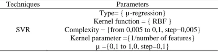
It is well known that the parameter settings could have a significant impact on the estimation accuracy of trained SDEE techniques. Therefore, building an accurate model requires selection of optimal values of its learning parameters [16]. However, finding optimal values is complicated task and various approaches have been proposed in the literature to address this issue, such as grid search (GS) [42], particle swarm optimization (PSO) [43] and genetic algorithm (GA) [39]. In order to enable SVR models, developed in this study, to achieve a higher prediction accuracy over the eight datasets used in SDEE, we employed grid search (GS) as optimization method combined with cross-validation procedure. The main idea behind the grid search method is that different pairs of parameters are tested and the one with the highest cross validation accuracy is selected. The major advantage of GS method is its high learning accuracy and the ability of parallel processing on the training of every SVR, because they are independent of each other. Although GS method can find the optimum parameters, the computational complexity is very big obviously, and the time spent is very large, especially for large sample data. In our case, we limited the search space to most promising values guided by previous studies [44]. Table 1 shows GS parameter for SVR models.
Table 1. Grid search parameter for SVR models
Techniques Parameters
SVR
Type= { µ-regression} Kernel function = { RBF } Complexity = {from 0,005 to 0,1, step=0,005}
Kernel parameter ={1/number of features} µ ={0,1 to 1,0, step=0,1}
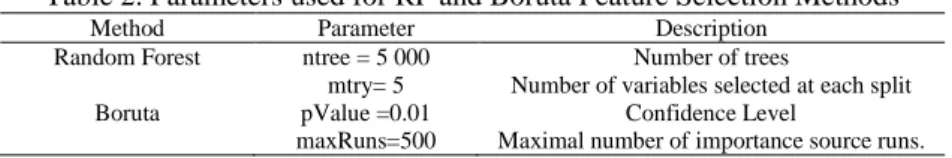
The GS method finds the best configuration of SVR models by evaluating every possible combination of Table 2 with respect to mean square error (MSE) based error function using 10-fold cross-validation approach. The best configuration of each technique that minimizes MSE is then selected. Note that the same range of parameter values were used for SVR with Boruta feature selection method. Regarding the parameters of random forest feature selection and Boruta algorithm were adjusted as shown in Table 3. In fact, these parameters do not have a significant impact on variable importance ranking except maxRuns parameter of Boruta method which should be increased in certain case to resolve attributes left Tentative by the algorithm.
Table 2. Parameters used for RF and Boruta Feature Selection Methods
Method Parameter Description
Random Forest ntree = 5 000
mtry= 5
Number of trees
Number of variables selected at each split
Boruta pValue =0.01
maxRuns=500
Confidence Level
Maximal number of importance source runs.
5. EXPERIMENTAL DESIGN
This section presents the experimental design of this study including: (1) the accuracy measures used to evaluate the proposed SVR models, (2) the description of the datasets used, and (3) the experimental process followed to construct and compare the different SVR models.
5.1. Accuracy measures
We employ the following criteria to assess and compare the accuracy of the effort estimation models. A common criterion for the evaluation of effort estimation models is magnitude of relative error (MRE), which is defined as
𝑀𝑅𝐸 = |(𝐸𝑓𝑓𝑜𝑟𝑡𝑎𝑐𝑡𝑢𝑎𝑙−𝐸𝑓𝑓𝑜𝑟𝑡𝑒𝑠𝑡𝑖𝑚𝑎𝑡𝑒𝑑
𝐸𝑓𝑓𝑜𝑟𝑡𝑎𝑐𝑡𝑢𝑎𝑙 )| (8)
The MRE values are calculated for each project in the dataset, while mean magnitude of relative error (MMRE) computes the average over N projects as follows:
𝑀𝑀𝑅𝐸 =1
𝑁∑ 𝑀𝑅𝐸𝑖
𝑁
𝑖=1 (9)
Generally, the acceptable target value for MMRE is 25%. This indicates that on the average, the accuracy of the established estimation models would be less than 25%. Another widely used criterion is the Pred(l) which represents the percentage of MRE that is less than or equal to the value l among all projects. This measure is often used in the literature and is the proportion of the projects for a given level of accuracy. The definition of Pred(l) is given as follows:
𝑃𝑟𝑒𝑑(𝑙) =𝑘
𝑁 (10)
Where N is the total number of observations and k is the number of observations whose MRE is less or equal to l. A common value for l is 0.25, which is also used in the present study. The Pred(0.25) represents the percentage of projects whose MRE is less or equal to 25%. The Pred(0.25) value identifies the effort estimates that are generally accurate whereas the MMRE is fairly conservative with a bias against overestimates [45-46]. For this reason, MdMRE has been also used as another criterion since it is less sensitive to outliers (10).
𝑀𝑑𝑀𝑅𝐸 = 𝑚𝑒𝑑𝑖𝑎𝑛(𝑀𝑅𝐸𝑖) (11)
5.2. Datasets
For this study, eight datasets, collected from different organizations and countries, were selected to evaluate the performance of SVR and SVR-RF techniques. A total of 1119 projects were used from three sources:
915 projects came from six datasets of PROMISE data repository which is a publicly available online data repository (Menzies et al. 2012) namely: Albrecht, COCOMO81, China, Desharnais, Kemerer and Miyazaki datasets.
151 projects selected from ISBSG R8 repository. In fact, this repository contains more than 2000 software projects described by more than 50 numerical and categorical attributes. The selected projects are the results of a data pre-processing study conducted by [47], the objective of which was to select data (projects and attributes), in order to retain projects with high quality. The first step of this study was to select only the new development projects with high quality data and using IFPUG counting approach. The second step was concerned by selecting an optimal subset of numerical attributes that are relevant to effort estimation and most appropriate to use as effort drivers in empirical studies.
53 Web projects from Tukutuku dataset [48]. Each Web application is described using 9 numerical attributes such as: the number of html or shtml files used, the number of media files and team experience. However, each project volunteered to the Tukutuku database was initially characterized
using more than 9 software attributes, but some of them were grouped together. For example, we grouped together the following three attributes: number of new Web pages developed by the team, number of Web pages provided by the customer and the number of Web pages developed by a third party (outsourced) in one attribute reflecting the total number of Web pages in the application (Webpages).
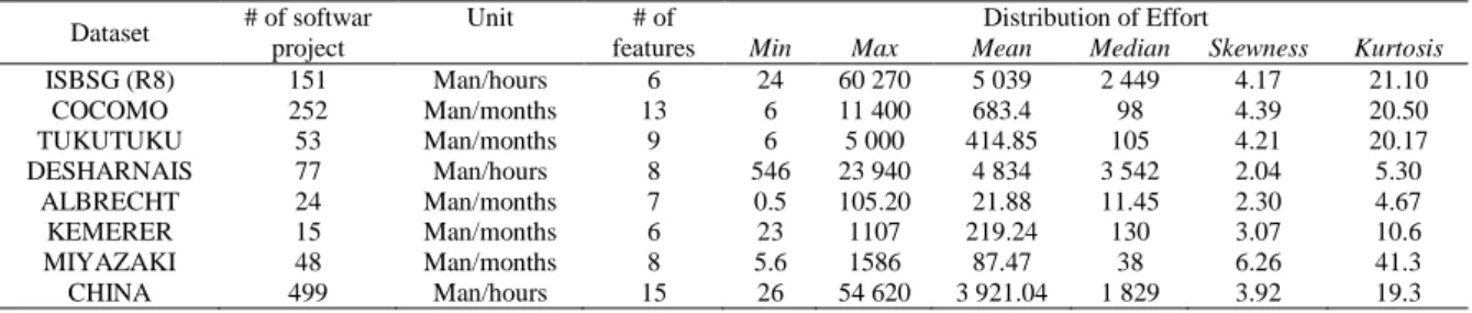
Table 3 summarizes descriptive statistics of the selected datasets, including size of dataset, effort unit, number of attributes, median, mean, minimum, maximum, skewness and kurtosis of effort. None of the selected datasets had a normally distributed effort as skewness values ranged from 2.04 to 6.26. This presents a challenge for researchers attempting to build accurate SDEE techniques [16, 49].
Table 3. Descriptive statistics of the eight datasets
Dataset # of softwar project Unit features # of Min Max Mean Distribution of Effort Median Skewness Kurtosis
ISBSG (R8) 151 Man/hours 6 24 60 270 5 039 2 449 4.17 21.10
COCOMO 252 Man/months 13 6 11 400 683.4 98 4.39 20.50
TUKUTUKU 53 Man/months 9 6 5 000 414.85 105 4.21 20.17
DESHARNAIS 77 Man/hours 8 546 23 940 4 834 3 542 2.04 5.30
ALBRECHT 24 Man/months 7 0.5 105.20 21.88 11.45 2.30 4.67
KEMERER 15 Man/months 6 23 1107 219.24 130 3.07 10.6
MIYAZAKI 48 Man/months 8 5.6 1586 87.47 38 6.26 41.3
CHINA 499 Man/hours 15 26 54 620 3 921.04 1 829 3.92 19.3
5.3. Validation method
A 30% holdout validation method was used to evaluate the generalization ability of the estimation models. So, the datasets were split randomly into two non-overlapping sets: training set containing 70% of data and testing set composed from 30% of the remaining data. The purpose of holdout evaluation is to test a model on different data to that from which it is learned. This provides less biased estimate of learning performance than all-in evaluation method.
6. EMPIRICAL RESULTS
This section reports and discusses the results of empirical experiments performed using SVR models designed in Section IV and following the building process illustrated in Figure 1. To carry out these empirical experiments, different R packages were used to develop an R prototype employed to construct the proposed models. In this way, e1071 package was used to build the SVR models and randomForest, and Boruta packages were used for feature selection methods.
6.1. Feature selection results
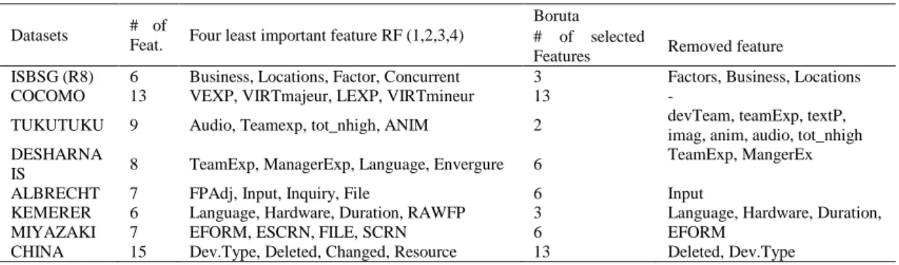
This subsection presents the results of the preprocessing step. Table 4 provides the four least important features generated by random forest, and the number of selected features and removed ones by Boruta method in each dataset. It can be seen from the data in Table 4 that the features rejected by Boruta are generally among the four least important feature identified by random forest, which is not surprising since Boruta algorithm is based on RF variable importance. However, Boruta method did not always remove the first least important feature. As example, for Albrecht dataset, it removed the second one (input) while the first least important feature is FPAdj. Concerning the number of the selected features, Boruta method selected almost at least 50% of features available in each dataset. The only exception was the case of Tukutuku dataset for which out of nine features, Boruta selected only two features. The single most striking result to emerge from the data is that all features of COCOMO dataset were deemed relevant and none of them was rejected.
Table 4. Number of selected features and removed ones in each dataset
Datasets # of
Feat. Four least important feature RF (1,2,3,4)
Boruta # of selected
Features Removed feature
ISBSG (R8) 6 Business, Locations, Factor, Concurrent 3 Factors, Business, Locations
COCOMO 13 VEXP, VIRTmajeur, LEXP, VIRTmineur 13 -
TUKUTUKU 9 Audio, Teamexp, tot_nhigh, ANIM 2 devTeam, teamExp, textP,
imag, anim, audio, tot_nhigh DESHARNA
IS 8 TeamExp, ManagerExp, Language, Envergure 6
TeamExp, MangerEx
ALBRECHT 7 FPAdj, Input, Inquiry, File 6 Input
KEMERER 6 Language, Hardware, Duration, RAWFP 3 Language, Hardware, Duration,
MIYAZAKI 7 EFORM, ESCRN, FILE, SCRN 6 EFORM
CHINA 15 Dev.Type, Deleted, Changed, Resource 13 Deleted, Dev.Type
6.2. Evaluation of SVR with FSS
The second step of the model building process uses the original and the reduced datasets to determine the best setup of the proposed SVR models. The best configuration is determined, as explained earlier, by a search grid to minimize the mean square error (MSE). Once the five SVR models were trained using training sets (70% of data), we evaluated the generalization capability of the five configurations of SVR models using testing sets (30%) over the eight datasets. The evaluation was based on the MMRE, MdMRE, and Pred(0.25) criteria. The complete empirical results obtained are shown in Tables 5-8. From data in Table 5, we notice that no SVR configuration gave the best Pred(0.25) value in all datasets. However, SVR-BFE_1 (removing only the least important feature) generated the best Pred in 6 out of 8 datasets and SVR-BFE_4 only came second by giving best value of Pred in 5 datasets. The SVR without FS and SVR with Boruta method produced best value of Pred only in one dataset: Kemerer and China respectively. The best value of Pred(0.25) was obtained by SVR-BFE_4 in China dataset (83.33).
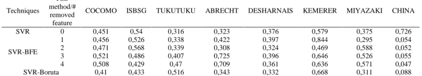
The results reported in Table 6 and Table 7 related to MMRE and MdMRE measures confirm the fact that no SVR configuration performed better than the other in all situation. Nevertheless, we can easily observe that the best values of MMRE and MdMRE are obtained with same datasets as those of Pred. So, the lowest errors were obtained with China dataset and highest errors were generated with ISBSG dataset. What is interesting about the data in these tables is that the values of MdMRE are far lower than those of MMRE especially in COCOMO, ISBSG, Tukutuku and Kemerer datasets. These latter findings agree with the values of skewness and kurtosis of these datasets that exhibit high level of asymmetry and of nonnormality.
Table 5. The results obtained in terms of pred(0.25) over the eight datasets Techniques
FSS method/#
removed features
COCOMO ISBSG TUKUTUKU ABRECHT DESHARNAIS KEMERER MIYAZAKI CHINA
SVR 0 30,263 26,667 31,25 28,571 21,739 20 35,714 15,333
SVR-BFE
1 36,842 31,111 37,5 42,857 30,435 20 42,857 81,333
2 32,895 24,444 37,5 42,857 34,783 20 21,429 81,333
3 31,579 24,444 37,5 42,857 34,783 0 21,429 80
4 36,842 31,111 12,5 42,857 39,13 0 28,571 83,333
SVR - Boruta 34,211 24,444 25 28,571 34,783 0 42,857 75,333
Table 6. The results obtained in terms of MMRE over the eight datasets Techniques
FSS method/#
removed feature
COCOMO ISBSG TUKUTUKU ABRECHT DESHARNAIS KEMERER MIYAZAKI CHINA
SVR 0 1,367 1,703 1,065 0,583 0,464 1,37 0,556 1,337
SVR-BFE
1 1,375 1,478 0,856 0,583 0,467 1,235 0,553 0,187
2 1,262 1,187 0,8 0,548 0,456 1,334 1,503 0,191
3 1,304 1,407 0,814 0,668 0,521 1,627 1,394 0,195
4 1,242 1,092 1,028 0,685 0,462 1,59 1,367 0,17
Table 7. The results obtained in terms of MdMRE over the eight datasets Techniques
FSS method/# removed feature
COCOMO ISBSG TUKUTUKU ABRECHT DESHARNAIS KEMERER MIYAZAKI CHINA
SVR 0 0,451 0,54 0,316 0,323 0,376 0,579 0,375 0,726
SVR-BFE
1 0,456 0,526 0,338 0,422 0,397 0,844 0,295 0,054
2 0,471 0,568 0,339 0,308 0,324 0,469 0,588 0,052
3 0,521 0,486 0,407 0,725 0,396 0,646 0,526 0,055
4 0,508 0,429 0,47 0,709 0,361 0,636 0,571 0,047
SVR-Boruta 0,41 0,433 0,516 0,343 0,332 0,668 0,311 0,088
Table 8. The Results obtained in terms of pred(0.25), MdMRE and MdMRE over the eight datasets Techniques FSS method / # removed feature Pred(0.25) MMRE MdMRE
SVR 0 26,192 1,056 0,461
SVR-BFE
1 40,367 0,842 0,417
2 36,905 0,910 0,390
3 34,074 0,991 0,470
4 34,293 0,955 0,466
SVR-Boruta 33,150 0,882 0,388
To sum up, the findings of this study suggest that the use of feature selection method in the preprocessing phase of the SVR model building can contribute significantly to improve the accuracy of effort estimates. In addition, the backward feature selection can generate better effort estimates than Boruta method.
7. CONCLUSION AND FUTURE WORK
This empirical study assessed the impact of feature selection methods on the accuracy of SVR models in SDEE. For this purpose, two wrapper feature selection methods were used to pre-process eight well-known datasets. The SVR models based on pre-processed datasets were compared to those built without feature selection. The SVR models were optimized using a grid search procedure. The performance of the proposed models was assessed using three accuracy measures through 30%holdout validation method. The results obtained showed that the SVR models with feature selection generated better estimation than the SVR constructed without feature selection methods. In addition, using the proposed backward feature elimination based on RF feature importance can leads to better accuracy than Boruta method. However, this study has only examined the SVR models based on one type of feature selection method. Therefore, it would be interesting to assess the impact of others feature selection methods on the accuracy of SVR models in SDEE.
REFERENCES
[1] B. W. Boehm, Software Engineering Economics. Prentice Hall PTR, 1981, p. 768.
[2] R. d. A. Araújo, A. L. I. Oliveira, and S. R. d. L. Meira, "A class of hybrid multilayer perceptrons for software development effort estimation problems," Expert Syst. Appl., vol. 90, pp. 1-12, / 2017.
[3] A. Zakrani and A. Idri, "Applying radial basis function neural networks based on fuzzy clustering to estimate web applications effort", International Review on Computers and Software, Article vol. 5, no. 5, pp. 516-524, 2010. [4] A. Zakrani, A. Namir, and M. Hain, "Investigating the use of random forest in software cost estimation", The
Second International Conference on Intelligent Computing in Data Sciences, Fès, 3-5 october, 2018.
[5] S. M. Satapathy, B. P. Acharya, and S. K. Rath, "Early stage software effort estimation using random forest technique based on use case points", IET Software, Article vol. 10, no. 1, pp. 10-17, 2016.
[6] A. Idri and I. Abnane, "Fuzzy Analogy Based Effort Estimation: An Empirical Comparative Study," in 17th IEEE International Conference on Computer and Information Technology, CIT 2017, 2017, pp. 114-121: Institute of Electrical and Electronics Engineers Inc.
[7] A. L. I. Oliveira, "Estimation of software project effort with support vector regression", Neurocomputing, Article vol. 69, no. 13-15, pp. 1749-1753, 2006.
[8] Q. Liu, J. Xiao, and H. Zhu, "Feature selection for software effort estimation with localized neighborhood mutual information", Cluster Computing, Article in Press pp. 1-9, 2018.
[9] Z. Chen, T. Menzies, D. Port, and B. Boehm, "Feature subset selection can improve software cost estimation accuracy," in 2005 Workshop on Predictor Models in Software Engineering, PROMISE 2005, 2005: Association for Computing Machinery, Inc.
[10] M. Azzeh, D. Neagu, and P. Cowling, "Improving analogy software effort estimation using fuzzy feature subset selection algorithm," in 30th International Conference on Software Engineering, ICSE 2008 - 4th International Workshop on Predictor Models in Software Engineering, PROMISE 2008, Leipzig, 2008, pp. 71-78.
[11] J. Li and G. Ruhe, "Software effort estimation by analogy using attribute selection based on rough set analysis", International Journal of Software Engineering and Knowledge Engineering, Article vol. 18, no. 1, pp. 1-23, 2008. [12] M. Hosni, A. Idri, and A. Abran, "Investigating heterogeneous ensembles with filter feature selection for software
effort estimation," in 27th International Workshop on Software Measurement and 12th International Conference on Software Process and Product Measurement, IWSM Mensura 2017, 2017, vol. Part F131936, pp. 207-220: Association for Computing Machinery.
[13] A. Idri and S. Cherradi, "Improving effort estimation of Fuzzy Analogy using feature subset selection," in 2016 IEEE Symposium Series on Computational Intelligence, SSCI 2016, 2017: Institute of Electrical and Electronics Engineers Inc.
[14] V. N. Vapnik, The nature of statistical learning theory. Springer-Verlag, 1995, p. 188.
[15] A. J. Smola and B. Schölkopf, "A tutorial on support vector regression," Statistics and Computing, journal article vol. 14, no. 3, pp. 199-222, August 01 2004.
[16] M. Hosni, A. Idri, A. Abran, and A. B. Nassif, "On the value of parameter tuning in heterogeneous ensembles effort estimation", Soft Computing, Article in Press pp. 1-34, 2017.
[17] G. Chandrashekar and F. Sahin, "A survey on feature selection methods," Computers & Electrical Engineering, vol. 40, no. 1, pp. 16-28, / 2014.
[18] R. Kohavi and G. H. John, "Wrappers for Feature Subset Selection," Artif. Intell., vol. 97, no. 1-2, pp. 273-324, / 1997.
[19] L. Breiman, "Random Forests," Machine Learning, vol. 45, no. 1, pp. 5-32, / 2001.
[20] F. Degenhardt, S. Seifert, and S. Szymczak, "Evaluation of variable selection methods for random forests and omics data sets," Briefings in Bioinformatics, pp. bbx124-bbx124, 2017.
[21] R. Genuer, J.-M. Poggi, and C. Tuleau-Malot, "Variable selection using random forests," Pattern Recognition Letters, vol. 31, no. 14, pp. 2225-2236, / 2010.
[22] M. B. Kursa and W. R. Rudnicki, "Feature Selection with the Boruta Package," 2010, vol. 36, no. 11, p. 13, 2010-09-16 2010.
[23] W. Zhang, Y. Du, T. Yoshida, Q. Wang, and X. Li, "SamEn-SVR: using sample entropy and support vector regression for bug number prediction," IET Software, vol. 12, no. 3, pp. 183-189, / 2018.
[24] Y. Cao, Z. Ding, F. Xue, and X. Rong, "An improved twin support vector machine based on multi-objective cuckoo search for software defect prediction," IJBIC, vol. 11, no. 4, pp. 282-291, / 2018.
[25] Z. Y. Ma, J. P. Wang, W. Zhang, Z. W. Shan, F. S. Liu, and K. Han, "Software reliability prediction based on optimized Support Vector Regression," in 2018 International Conference on Big Data and Computing, ICBDC 2018, 2018, pp. 129-133: Association for Computing Machinery.
[26] X. Jin, Z. Liu, R. Bie, G. Zhao, and J. Ma, "Support vector machines for regression and applications to software quality prediction," in ICCS 2006: 6th International Conference on Computational Science vol. 3994 LNCS - IV, ed. Reading: Springer Verlag, 2006, pp. 781-788.
[27] A. Garcia-Floriano, C. L. Martín, C. Yáñez-Márquez, and A. Abran, "Support vector regression for predicting software enhancement effort," Information & Software Technology, vol. 97, pp. 99-109, / 2018.
[28] P. L. Braga, A. L. I. Oliveira, and S. R. L. Meira, "A GA-based feature selection and parameters optimization for support vector regression applied to software effort estimation," in 23rd Annual ACM Symposium on Applied Computing, SAC'08, Fortaleza, Ceara, 2008, pp. 1788-1792.
[29] A. Corazza, S. D. Martino, F. Ferrucci, C. Gravino, F. Sarro, and E. Mendes, "How effective is Tabu search to configure support vector regression for effort estimation?" 2010. Available: http://doi.acm.org/10.1145/1868328.1868335
[30] A. Corazza, S. D. Martino, F. Ferrucci, C. Gravino, and E. Mendes, "Investigating the use of Support Vector Regression for web effort estimation," Empirical Software Engineering, vol. 16, no. 2, pp. 211-243, / 2011. [31] J. C. Lin and C. T. Chang, "Genetic algorithm and support vector regression for software effort estimation," in 2011
International Conference on Material Engineering, Chemistry, Bioinformatics, MECB2011 vol. 282-283, ed. Wuhan, 2011, pp. 748-752.
[32] J. C. Lin, C. T. Chang, and S. Y. Huang, "Research on software effort estimation combined with genetic algorithm and support vector regression," in 2011 International Symposium on Computer Science and Society, ISCCS 2011, Kota Kinabalu, 2011, pp. 349-352.
[33] A. Corazza, S. D. Martino, F. Ferrucci, C. Gravino, F. Sarro, and E. Mendes, "Using tabu search to configure support vector regression for effort estimation," Empirical Software Engineering, vol. 18, no. 3, pp. 506-546, / 2013.
[34] L. Song, L. L. Minku, and X. Yao, "The potential benefit of relevance vector machine to software effort estimation," in 10th International Conference on Predictive Models in Software Engineering, PROMISE 2014, Turin, 2014, pp. 52-61: Association for Computing Machinery.
[35] K. Iwata, E. Liebman, P. Stone, T. Nakashima, Y. Anan, and N. Ishii, "Bin-based estimation of the amount of effort for embedded software development projects with support vector machines," in Studies in Computational Intelligence vol. 614, ed: Springer Verlag, 2016, pp. 157-169.
[36] D. Novitasari, I. Cholissodin, and W. F. Mahmudy, "Hybridizing PSO with SA for optimizing SVR applied to software effort estimation", Telkomnika (Telecommunication Computing Electronics and Control), Article vol. 14, no. 1, pp. 245-253, 2016.
[37] T. R. Benala and R. Bandarupalli, "Least Square Support Vector Machine in Analogy-Based software development effort estimation," in 2016 IEEE International Conference on Recent Advances and Innovations in Engineering, ICRAIE 2016, 2017: Institute of Electrical and Electronics Engineers Inc.
[38] A. Tiwari and A. Chaturvedi, "Class partition approach for software effort estimation using support vector machine," in 2016 IEEE Uttar Pradesh Section International Conference on Electrical, Computer and Electronics Engineering, UPCON 2016, 2017, pp. 653-659: Institute of Electrical and Electronics Engineers Inc.
[39] A. L. I. Oliveira, P. L. Braga, R. M. F. Lima, and M. L. Cornélio, "GA-based method for feature selection and parameters optimization for machine learning regression applied to software effort estimation", Information and Software Technology, Conference Paper vol. 52, no. 11, pp. 1155-1166, 2010.
[40] A. Corazza, S. D. Martino, F. Ferrucci, C. Gravino, and E. Mendes, "Using Support Vector Regression for Web Development Effort Estimation," 2009. Available: https://doi.org/10.1007/978-3-642-05415-0_19
[41] A. Corazza, S. D. Martino, F. Ferrucci, C. Gravino, and E. Mendes, "Applying support vector regression for web effort estimation using a cross-company dataset," 2009. Available: http://doi.acm.org/10.1145/1671248.1671267 [42] X. Ma, Y. Zhang, and Y. Wang, "Performance evaluation of kernel functions based on grid search for support
vector regression," 2015. Available: https://doi.org/10.1109/ICCIS.2015.7274635
[43] H. Zhang, M. Wang, and X. Huang, "Parameter Selection of Support Vector Regression Based on Particle Swarm Optimization," 2010. Available: https://doi.org/10.1109/GrC.2010.121
[44] P. L. Braga, A. L. I. Oliveira, and S. R. L. Meira, "Software effort estimation using machine learning techniques with robust confidence intervals," in 7th International Conference on Hybrid Intelligent Systems, HIS 2007, Kaiserslautern, 2007, pp. 352-357.
[45] T. Foss, E. Stensrud, B. Kitchenham, and I. Myrtveit, "A Simulation Study of the Model Evaluation Criterion MMRE," IEEE Trans. Software Eng., vol. 29, no. 11, pp. 985-995, / 2003.
[46] A. Idri, I. Abnane, and A. Abran, "Evaluating Pred(p) and standardized accuracy criteria in software development effort estimation", Journal of Software: Evolution and Process, Article vol. 30, no. 4, 2018, Art. no. e1925. [47] F. A. Amazal, A. Idri, and A. Abran, "Software development effort estimation using classical and fuzzy analogy: A
cross-validation comparative study",, International Journal of Computational Intelligence and Applications, Article vol. 13, no. 3, 2014, Art. no. 1450013.
[48] E. Mendes and B. A. Kitchenham, "Further Comparison of Cross-Company and Within-Company Effort Estimation Models for Web Applications," presented at the 10th International Symposium on Software Metrics, Chicago, Illinois, USA, 2004.
[49] M. Azzeh, A. B. Nassif, and L. L. Minku, "An empirical evaluation of ensemble adjustment methods for analogy-based effort estimation," Journal of Systems and Software, vol. 103, pp. 36-52, 2015.
BIOGRAPHIES OF AUTHORS
Abdelali Zakrani is an assistant professor at Hassan II university at Casablanca, He received the B.Sc. degree in Computer Science from Hassan II University, Casablanca, Morocco, in 2003, and his DESA degree (M.Sc.) and Ph. D. in the same major from University Mohammed V, Rabat, in 2005 and 2012 respectively. His research interests include software cost estimation, software metrics, fuzzy logic, neural networks, decision trees.
Mustapha Hain is an associate professor at Hassan II university at Casablanca, He received the B.Sc. degree in Electrical engineering from Hassan II University, Casablanca, Morocco, in 2000, and his DESA degree (M.Sc.) and Ph. D. in Computer science from University Hassan II, Casablanca, in 2006 and 2011 respectively. His research interests include model driven architecture, software engineering, information systems.
Ali Idri is a Professor at Computer Science and Systems Analysis School (ENSIAS, University Mohamed V, Rabat, Morocco). He received DEA (Master) (1994) and Doctorate of 3rd Cycle (1997) degrees in Computer Science, both from the University Mohamed V of Rabat. He has received his Ph.D. (2003) in Cognitive Computer Sciences from University of Quebec at Montreal. He is the head of the Software Project Management research team since 2010. He is the chairman of the 10th International conference in Intelligent Systems: Theories and Application a (SITA 2015) and he serves as a member of program committee of major international journals and conference. His research interests include software effort/cost estimation, software metrics, software quality, computational intelligence in software engineering, datamining, e-health. He has published more than 150 papers in several international journals and conferences