Sharif University of Technology
Scientia IranicaTransactions E: Industrial Engineering www.scientiairanica.com
A new proactive-reactive approach to hedge against
uncertain processing times and unexpected machine
failures in the two-machine ow shop scheduling
problems
D. Rahmani
Department of Industrial Engineering, K. N. Toosi University of Technology, Tehran, Iran. Received 20 October 2015; received in revised form 21 February 2016; accepted 19 July 2016
KEYWORDS Disruption; Robustness; Stability; Nervousness; Flow shop; Proactive-reactive approach.
Abstract.In this paper, a proactive-reactive approach has been considered for achieving stable and robust schedules despite uncertain processing times and unexpected machine failures in a two-machine ow shop system. In the literature, Surrogate Measures (SMs) have been developed for achieving stable and robust solutions against the occurrence of stochastic disruptions. These measures proactively provide an approximation of the real conditions of the system in the event of a disruption. Because of the discrepancies of these measures with their real values, a dierent approach is developed in this paper in a two-step structure. First, an initial robust schedule is produced and then, based on a multi-component measure, an appropriate reaction is adopted against unexpected machine failures. Computational results indicate that this method produces better solutions compared to the other two classical scheduling approaches considering their eectiveness and performance.
© 2017 Sharif University of Technology. All rights reserved.
1. Introduction
In the classical scheduling problems, it is assumed that the information about all jobs and their characteriza-tions is known initially, and the objective is usually to optimize some classical performance measures such as tardiness and makespan under deterministic assump-tions [1]. However, in dynamic manufacturing envi-ronments, the scheduling problems with uncertainty are addressed. In stochastic scheduling problems, the solving approaches often try to optimize the expected value or some other probabilistic measure of the ob-jective function [2]. In uncertain scheduling problems, other measures are proposed to incorporate the uncer-tainty [3]. Ouelhadj and Petrovic [4] presented a survey
*. Tel.: +98 21 84063357; Fax: +98 21 88674858 E-mail address: [email protected]
on dynamic scheduling in manufacturing systems. In fact, because of random disruptions that may occur in the system, additional measures (such as robustness and stability) should be considered. Some disruptions that may occur in real-world manufacturing systems include:
Machine breakdowns;
Cancellation of orders;
Changes in delivery times;
Uncertain due dates;
Uncertain processing times;
Equipment overhaul;
Addition or removal of operations.
In practice, the scheduling process starts by de-termining an initial schedule. Then, when a disruption
arises, the initial schedule should be revised in order to maintain its feasibility and quality. The type of schedule that is actually carried out in shops is known
as real schedule. Obviously, real schedule can be
dierent from the initial schedule because of occurrence of unexpected events. This depends on the level of failures, disruptions, and the changes of the setting. In the literature, there are two strategies for obtaining high system performance from the real schedule after any disruption. These strategies are called reactive scheduling and proactive scheduling.
The reactive scheduling approach does not ini-tially consider uncertainty, but revises and improves the schedule when unpredicted events occur. In fact, reactive scheduling is a method that provides good reactions when encountering failure and disruption. This reaction can modify the initial schedule or gen-erate a completely new schedule. However, proactive scheduling strategy considers future disruptions when generating an initial schedule. It actually seeks a schedule that also controls the eects of future disrup-tions by some predictive performance measures such as robustness and stability. Optimization of stability is concerned with the deviation of the real schedule from the initial schedule. Optimization of robustness is concerned with deference in terms of objective function between initial and modied schedules [5]. Of course, a combined proactive-reactive approach can also be considered [6].
In this paper, a two-stage proactive-reactive method is presented for coping with uncertain and unexpected events. In the rst stage, it is attempted to produce an initially robust schedule by using the
robust optimization approach. The initial robust
schedule counters the uctuations of processing times. In the second stage, when an unexpected disruption occurs (i.e., machine failure), an appropriate reaction is adapted to rescheduling.
This paper is organized in the following manner. In Section 2, the related technical literature is reviewed and a brief description of robust optimization approach is presented. The main two-step approach of the paper is presented in Section 3. In the rst step, a robust model of two-machine ow shop scheduling problem has been presented and solved, and in the second step, the appropriate reactive approach has been described. Computational results and relevant comparisons have been presented in Section 4. Finally, conclusions and recommendations for future studies have been presented in the last section.
2. Literature review
Flow shop is one of the most practical and real-world production environments, especially in assembly facilities [7]. Some researchers including Fattahi et
al. [8] proposed mathematical models to formulate the ow shop environment and some heuristics to solve the problem.
In order to decrease the eect of uncertain pro-cessing times, some researchers considered a specic distribution function for them and solved the prob-lem based on the stochastic optimization approach. Some other researchers used the robust optimization approach so that this approach could improve the performance of the presented schedule by facing the uctuations of uncertain processing times concerning
all possible future scenarios. Proactive scheduling
methods that deal with the future uctuations of uncertain parameters using the robust optimization approach are presented in [9-12].
Considering disruptions and unexpected events in scheduling systems, the researchers either used iteration based simulation methods [13] or attempted to develop robust and stable schedules to face these disruptions. Wu et al. [14] considered increase in stability of the single-machine rescheduling problem with machine breakdowns. They rescheduled the jobs in response to machine failures so that the minimum makespan could achieve a high scheduling stability. Leon et al. [15] studied the issue of robustness in the job shop environment. They assumed that the times of failure and repairing were known values, and makespan was the shop performance measure that should be minimized. For analysis of the eects of machine failures and changes of the processing times, the authors proposed a slack time based robustness measure. The most promising robustness measure is expressed as:
Zr=1(s) = MSmin RD3(s); (1)
where MSmin is the makespan of schedule s and
RD3(s) is the average slack in schedule s. Lawrence and Sevelle [16] studied the performance of the simple dispatching heuristics against the algorithmic solution techniques in a job shop environment with uncertain processing times. A similar study was undertaken by Sabunkuglu and Karabuk [17] in which they showed that the dispatching rules for interruptions were more robust than the optimum search algorithms for oine schedules. Jensen [18] generated robust schedules in a job shop environment with respect to machine break-downs for minimizing makespan. Jensen's idea was based on the principle that the robust optimal solution was found in the wider regions of the distribution (objective) function, while the non-robust and fragile optimal solutions were located on the narrow peaks of the distribution function. In fact, he considered the neighborhood-based robustness measure for including the schedule s and all the achievable schedules. His formula is as follows:
ZMSnib(s) =
1 jN1(s)j
X
s02N1(s)
MSmin(s0); (2)
where MSmin(s0) is the makespan of schedule s0.
The neighborhood N1(s) contains s and all feasible
schedules that can be created from s by interchange of two consecutive operations on the same machine. Goren and Sabuncuoglu [19] investigated the problem of robust and stable schedule with random failures in a single-machine environment. They presented two surrogate measures for robustness and stability, and used the tabu search algorithm to solve the problem. Sotskov et al. [20] presented a number of approaches based on interval processing times for the evaluation of robustness and stability in a single-machine envi-ronment. Bouyahia et al. [21] proposed a probable comprehensive approach for the robustness design of pre-scheduling, which assumed that the number of jobs to be processed on parallel machines was a random variable. They studied the total weighted ow time as an objective function. Ghezail et al. [22] proposed a qualitative graphical approach for responding to the disruptions in the ow shop problem. They proposed a graphical approach that helped the decision maker to observe the consequences of random failures and to choose the best sequence. Al-Hinai and ElMekkawy [23] produced proactive robust and stable solutions for the exible job shop scheduling problem with random failures. They introduced a new methodology that combined the approach of insertion of non-idle time and a hybrid genetic algorithm proposed in [24].
Based on the literature, the researchers consid-ered stability and robustness separately to face the
stochastic disruptions in scheduling problems. To
produce robust and stable solutions, the true value of uncertain parameters should be determined. However, since the exact values of these parameters are not specied from the start, either iteration based time-consuming simulation methods or surrogate measures are used in the literature to obtain robust and stable solutions. Because of the discrepancies between these measures and their true values, they may not show the true performance of the system. We proposed a new proactive-reactive approach instead of SMs to overcome their weaknesses and achieve good-quality solutions. We also considered a new practical measure called \ner-vousness" in the two-machine ow shop scheduling in addition to the stability and robustness. Accordingly, a multi-criteria measure was presented in the reactive stage of the proposed method. In the following, the structure of the robust optimization approach used to formulate our considered problem is explained [25]. Statement of contribution
An uncertain two-machine ow shop problem is
considered;
A two-stage method is presented to reduce the
eects of uncertainty and disruption;
A robust model is developed to create an initial
ro-bust schedule to overcome the uncertain processing times;
A new measure called \NERS value" is proposed to
apply a good reaction after a machine failure;
Four critical factors are included in the proposed
measure to select the best method for rescheduling after a disruption;
Multiple methods to evaluate the performance of the
proposed method are considered.
Robust optimization approach: The aim of the robust optimization approach is to get a set of solutions for the problem that remains robust despite the changes that may occur in the real values of data and input pa-rameters (shown by a set of scenarios). The structure of robust optimization is briey explained in the following section. Consider the following linear model:
min cTx + dTy; (3)
subject to:
Ax = b; (4)
Bx + Cy = e; (5)
x; y 0;
where x is the vector of decision variables and y is the vector of control variables. B and C are coecient vectors and e is the right hand side vector. Assume that there exists a set of scenarios, = f1; 2; :::; ~g. Under each scenario, , the uncertain coecients are dened
as fd; B; C; eg and the probability of occurrence
of each scenario is p (P
p = 1). Each scenario
comprises a set of data that may occur in the future. Since y (vector of control variables) is determined in the constraint depending on the scenario that occurs,
it is dened as y. Due to the existence of uncertain
parameters, the model may become infeasible for some
scenarios; in this case, is the degree of infeasibility
of the model under scenario . If the model is feasible,
then = 0. Thus, is an error vector that will
mea-sure the infeasibility allowed in the control constraints under scenario . The ultimate goal of this approach is the optimization of the problem with two kinds of robustness: solution robustness, which guarantees a near-optimum solution for all the scenarios, and model robustness, which guarantees the problem solution to be feasible for all the possible scenarios. Therefore, the robust model is made as follows:
subject to:
Ax = b; (7)
Bx + Cy + = e 8 2 ; (8)
x 0; y 0; 0 8 2 : (9)
In Constrain (6), (:) denotes the solution robustness and (:) is the model robustness. In fact, (:) is a penalty function for the solution possibility, which is used to penalize the deviations of control constraints under some of the scenarios. Also, coecient ! estab-lishes the equilibrium between the solution robustness and model robustness. Constraint (7) is the structural constraint and there is no noise. Constraint (8) is the control constraint that contains noisy coecients. Con-straint (9) ensures non-negative values for variables.
The rst term in the objective function can be
dened with a random variable such as = cTx + dTy
that takes the value = cTx+dT
ywith probability
p under scenario . To dene (:), Mulvey et al. [11]
used the following relation:
(:) =X
=2
p+ X
2
p X
02
p0
0
!2
; (10) in which the solution has a lower sensitivity to the changes of uncertain data as increases. However, since this term is quadratic, its solving will be com-plicated; due to this, Yu and li [26] dened another term for (:) as:
(:) =X
=2
p+ X
2
p X
02
p0
0
: (11) But since this term is linear, by dening a non-negative deviational variable, the problem is converted to a linear model as follows:
(:) =X
=2
p+ X
2
p X
02
p0
0
+2; (12)
subject to:
X
02
p0
0
+ 0; 8 2 ;
0; 8 2 : (13)
3. Proposed method
In this paper, a two-machine ow shop problem with uncertain job processing times is considered. There
is some information about uncertain processing times, and they are estimated by scenarios. In addition to un-certain processing times, unexpected failures may occur in the future; but there is no predictive information in this regard. Therefore, in the rst stage of the proposed method, unexpected machine failure is not considered, because they are completely unexpected events and there is no information to formulate them. Hence, in the rst stage, an initial solution for scheduling is obtained by only considering the problem with uncertain processing times. The robust optimization approach is used in order for this initial solution to be a robust solution as well. Actually, to reduce the eect of uncertainty on processing times, which is a random disruption in the future, the problem is formulated using the robust optimization approach, rstly, in an attempt to produce robust initial solutions. After an initially robust schedule is determined, the machines start to process the jobs according to this schedule. However, each machine may break down during the processing of jobs. Therefore, in the second stage, a reactive approach is presented to deal with such unexpected failures. In fact, when a machine failure occurs, an appropriate reaction should be adopted
to handle this disruption. Suppose that dierent
reactions, like regeneration, right shifting, or any other heuristic reaction can be implemented following the failure. When adopting a reactive response, a multi-component measure is dened based on a clas-sic objective and three other performance measures. This measure helps us choose the most appropriate reaction to counter the eect of machine failures. A owchart of our proposed approach is presented in Figure 1.
3.1. Proactive scheduling stage
In this stage, only the problem with uncertain pro-cessing times is considered. The robust optimization approach is used to formulate the two-machine ow shop problem to reduce the eects of uctuations of the processing times in the future. Consider a set J = f1; 2; :::; ng of n independent jobs that require processing on each of the two machines. Assume
that there exists a limited set of f1; 2; :::; ~g. A
robust solution is proactively generated as an initial schedule.
3.1.1. Notations Indices:
n The number of jobs
; 0 Indices for scenarios
r Index for positions f1; 2; :::; ng
j Index for jobs f1; 2; :::; ng
Figure 1. The owchart of the proposed proactive-reactive method.
Parameters: t
ij The processing time of job j on
machine i under scenario
p The probability for occurrence of
scenario
M A large number
Variables:
xijr 1 if the job j is processed on machine i
in the position r; 0 otherwise
CP
ijr The predictive completed time of job
j on the machine i in the position r under scenario
3.1.2. Proactive robust model
Now, the considered problem is formulated based on the robust optimization approach described in the previous section. The noteworthy point is that in this model, due to the unequal form of the existing constraints, it is not necessary to dene parameter
and function (1; 2; :::; ~) to guarantee solution
robustness. Therefore, the issue of creating a balance between solution robustness and model robustness no longer exists. Therefore, our developed robust model is as follows:
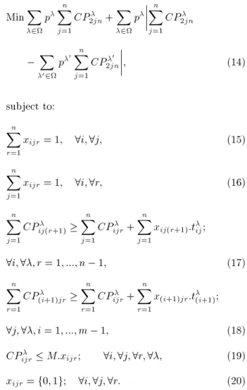
MinX
2
pXn
j=1
CP
2jn+
X
2
pXn j=1
CP
2jn
X
02
p0Xn
j=1
CP0
2jn
; (14)
subject to:
n
X
r=1
xijr= 1; 8i; 8j; (15)
n
X
j=1
xijr= 1; 8i; 8r; (16)
n
X
j=1
CP
ij(r+1) n
X
j=1
CP
ijr+ n
X
j=1
xij(r+1):tij;
8i; 8; r = 1; :::; n 1; (17)
n
X
r=1
CP
(i+1)jr n
X
r=1
CP
ijr+ n
X
r=1
x(i+1)jr:t(i+1);
8j; 8; i = 1; :::; m 1; (18)
CP
ijr M:xijr; 8i; 8j; 8r; 8; (19)
xijr= f0; 1g; 8i; 8j; 8r: (20)
To linearize the objective function, a method is used
and the dened parameter has been described in
the previous section [26]. Therefore, we have:
MinX
2
pXn
j=1
CP
2jn+
X
2
pXn
j=1
CP
2jn
X
02
p0Xn
j=1
CP0
2jn
+ 2
; (21)
Xn
j=1
CP
2jn+
X
02
p0Xn
j=1
CP0
2jn 0; 8:
(22) Thus, Objective (21) and Constraints (22) ensure that the optimal schedule conforms to the denition of ro-bust schedule based on a linear model. Constraints (15) to (20) are necessary scenario-based constraints in a two-machine ow shop system to calculate appropriate makespan. These constraints guarantee that the robust schedule is feasible.
3.2. Reactive scheduling stage
Assume that in the rst stage, an initial robust schedule is determined. The machines may break down during
the processing of jobs unexpectedly. Suppose that
machine i fails at time tf. In this case, the main point
is to choose an appropriate heuristic as a good reaction after this failure. The important point that should be mentioned is that the proposed approach to respond to the machine failure is a reactive one. Therefore, there is no need to know the distribution function of the failure occurrence time and repair duration.
Suppose that a set of heuristic methods, =
fH1; H2; :::; Hhg, exists, which can be used after the
occurrence of failure. These heuristic methods can be the right shifting, regeneration, or any other heuristic. In this research, a multicomponent measure is dened to choose the most appropriate heuristic method from the set . This measure is dened based on a classi-cal objective and three other performance measures. The considered classical objective in this research is makespan that indicates scheduling eectiveness. Other performance measures include robustness, sta-bility, and nervousness that control the unexpected disruptions. This measure is called \NERS value" (including Nervousness, Eectiveness, Robustness, and Stability). These components are described in the following subsections.
3.2.1. Scheduling eectiveness
This measure indicates the degree of optimality of a schedule. In this paper, this criterion is measured by the classical objective \makespan". It should be mentioned that because of disruptions such as machine failures in the system, the real completion time of aected jobs may change. The stochastic variable
CRijris dened as the real completion time of job j on
machine i at position r. Therefore, in a two-machine
ow shop system, PjCR2jn is the real makespan for
the realized schedule that explains scheduling eective-ness.
3.2.2. Robustness
The robustness of a schedule refers to its ability to perform well under dierent operational environments. In fact, robustness is concerned with the dierence in objective function values before and after a disruption. It refers to the insensitivity of scheduling performance to the disruptions. Some robustness measures are based on the actual performance of the realized sched-ules, and some are based on regret. [3]. In this research, this measure is dened as the closeness of the realized schedule performance to the initial schedule.
It should be mentioned that in the rst stage, in order to determine the initial schedule, the processing
times were estimated as scenarios. In fact, some
issues such as the condition of machines, the state of operators, the environmental conditions, etc. aect processing times and the real states of these issues would be determined only at schedule execution time.
A nite number of scenarios (three scenarios) were considered to dene the uncertain processing times to obtain a robust initial schedule. As mentioned earlier, in robust optimization approach, one of these scenarios would occur in future. During the planning of an initial schedule, the real scenario that will really occur in the system is not determined. But, when the production process begins, before a disruption, one or more jobs have been processed on machines, and so we can nd out which scenario has occurred. In fact, the compatible scenario with these completed jobs has been
determined. Considering this notion, suppose 00 2
is the scenario that has really occurred after the start of jobs processing. In this case, the real completion times without considering unexpected failures are specied
based on the scenario 00 2 . Based on this matter
and the denition of robustness (absolute deviation in system performance), the robustness measure is calculated as follows:
Robustness measure :
X
j
CR2jn
X
j
CP00
2jn
;(23)
P
jCR2jn is the real makespan of the perturbed
schedule and PjCP00
2jn is the predictive makespan
according to the initial schedule that is determined
according to the occurred scenario 00.
3.2.3. Stability
It is the degree of rearrangement of jobs (sequence, start-times, and so on) after rescheduling [27]. In this paper, this measure is dened as the dierence between the completion times of the jobs in the initial schedule and the realized ones [23]. When a disruption occurs, the real sequence may change after a needed rescheduling. This matter may lead to additional costs, including the costs of reallocation of tools and equip-ment, reordering raw materials, etc. However, when the real schedule is closer to the initial one, these costs are reduced and stability increases. On the other hand, stability is concerned with the dierence between initial and realized schedules themselves rather than between their performances. Therefore, stability measure is dened as absolute deviation in job completion times as follows:
Stability measure :X2
i=1 n
X
j=1 n
X
r=1
jCRijr CPijr00j;
(24)
CRijr is the real completion time of job j on the
machine i in position r, and CP00
ijr is the predictive
completion time of job j on machine i in position r
under occurred scenario 00.
3.2.4. Nervousness
Schedules are intrinsically nervous and fragile with some unexpected information. This information is not
known a priori in the planning phase and is revealed over time; thus, dynamic or on-line scheduling tech-niques are usually used [27,28]. To show the inuence of nervousness in scheduling problems, another approach is developed in this paper and a new measure, such as the measure of robustness or stability, is dened. This measure includes the eect of frequency of rescheduling in the system after disruptions. When a disruption occurs in a system and the sequence of jobs changes after rescheduling, the change in the sequence causes nervousness in the system. In fact, internal system components, like the operators, will fall into disarray due to change in the sequence and the more this rescheduling frequency, the higher the nervousness of the system will be. Therefore, when the sequence of one or several jobs in the real schedule changes relative to the initial schedule, the system becomes turbulent and chaotic. In this paper, the concepts of instability and nervousness are dierentiated. For example, the jobs may be right-shifted after a failure. In this way, due to the change in the completion time of jobs, the stability measure will be a positive number while the nervousness is zero, because the sequence of jobs does not change.
It is assumed that P O00
ij is the predictive position
of job j on machine i under occurred scenario 00 and
ROijis the real position of job j on machine i following
a failure. A variable is dened as follows:
Nij = 1 if ROij 6= P O
00
ij ; and Nij = 0 otherwise:
In fact, if the position of job j in the real schedule
is dierent from the predictive one, then Nij = 1.
Now, variable T CO is dened as the total change in position of jobs following an unexpected failure;
therefore, T CO = P2i=1Pnj=1Nij. T CO describes
nervousness of scheduling.
3.2.5. NERS value as a selector measure
The NERS value is a multicomponent measure for the selection of a suitable heuristic to deal with failure of machines. The nal denition of NERS value based on the above dened components is as follows:
Selection measure = (Eectiveness)
+ (Robustness measure) + v (Stability measure)
+' (Nervousness): (25)
The existing coecients in this measure indicate the importance of each component. These values are de-termined by the decision makers of the system, such as managers. Thus, in the proposed reactive stage, when a failure occurs, rst, the values of these coecients are determined by the managers of the production system. To determine the weight of each measure,
a sensitivity analysis approach can be used, such as the research presented in [27]. They similarly dene a comparison metric with four components for comparing deterministic, robust, and online scheduling. They use a sensitivity analysis to determine the weight of each component. Therefore, in a real case, the analyst can consider dierent amounts for the classical measure and other three components and the manager can choose the better one according to her/his preferences. Moreover, there are many approaches for determining preference weights in multi-criteria decision making, such as the eigenvector method, weighted least-square method, entropy method, and linear programming technique for multidimensional analysis of preference (LINMAP). The readers are referred to Hwang and Yoon [29] for more information. The denition of NERS value is as follows:
NERS valueH =
(P
jCR2jn)H
maxH2(PjCR2jn)H
+
P
jCR2jn PjCP
00
2jnH
maxH2PjCR2jn PjCP2jn00H
+v
P2
i=1
Pn
j=1
Pn
r=1CRijr CP
00
ijrH
maxH2P2i=1Pnj=1Pnr=1CRijr CPijr00H
+'
T COH
maxH2T COH
; (26)
+ + v + ' = 1: (27)
A set of heuristics can be compared using the NERS value. In fact, after determining the weights, the NERS value is calculated for each heuristic, such as right shifting, regeneration, etc., and the heuristic with the lowest amount of NERS value is selected as a proper reaction to respond to the disruption. The terms in Eq. (25) will be normalized to enable a reasonable comparison between heuristics [27].
3.3. Solution methods
There are dierent heuristics to deal with unexpected disruptions. More common methods in the literature are regenerations and right shifting methods that are explained in the following subsections.
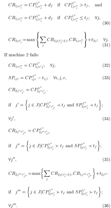
3.3.1. Right shifting
One of the simplest reactions, which are commonly implemented in the literature, following the occurrence of a disruption is right shifting. In this approach, when a failure happens, the jobs are processed with the same previous sequence following the repair of failed machine. In this case, the completion time of jobs will be shifted to right within the repair duration
(df). The schedule may be less stable in this method
because the real completion time of jobs may change signicantly. The advantage of this method is that, due to no change in the sequence, the costs of setup and startup will be less and the system nervousness will be zero. As mentioned earlier, when the man-ufacturing process begins, we are absolutely certain about which scenario has occurred. Considering this
notion, suppose that 002 is the scenario which has
really occurred after the start of the jobs processing. Now, assume that the system has a failure and the scheduled activities are shifted to the right following the failure. Two hypothetical machine failures are shown in Figure 2. Assume that j1, j2, and j3 are
scheduled based on occurred scenario 00 according to
Figure 2(a). Figure 2(b) and (c) are presented machine failures in dierent times for machine 1 and machine 2, respectively. Figure 2 shows the steps of right shifting method following the considered failures.
In general, with a repair duration df and occurred
scenario 00, the value of real completion time of jobs
is obtained as follows: r0
j = fr 2 njx2jr= 1g; 8j; (28)
r00
j = fr 2 njx1jr= 1g; 8j: (29)
If machine 1 fails:
Figure 2. (a) An initial schedule. (b) Right shifting following a failure on machine 1. (c) Right shifting following a failure on machine 2.
CR1jr00 j = CP
00
1jr00
j + df if CP
00
1jr00
j > tf; and
CR1jr00 j = CP
00
1jr00
j + df if CP
00
1jr00
j tf; 8j;
(30) CR2jr0
j=max
8 < :
X
j
CR2j(r0
j 1); CR1jr00j
9 =
;+t2j; 8j:(31)
If machine 2 fails: CR1jr00
j = CP
00
1jr0j; 8j; (32)
SPijr = CPijr00 tij; 8i; j; r; (33)
CR2j0r0 j0 = CP
00
2j0r0 j0:
if j0 =
j 2 JjCP00
2j0r0
j0 tf and SP
00
2jr0 j tf
;
8j0; (34)
CR2j00r0
j00 = CP
00
2j00r0 j00
if j00=j 2 JjCP00
2jr0
j tf and SP
00
2jr0 j tf
;
8j00; (35)
CR2j000r0
j00=max
X
j
CR2j(r0
j 1); CR1j000r00j00
+t2j000
if j000 =j 2 JjCP00
2jr0
j tf and SP
0
2jr0 j tf
;
8j000: (36)
3.3.2. Regeneration
Another method that can be adopted as a rescheduling method following a failure is regeneration heuristic. It reschedules the set of jobs not processed before the rescheduling point and aected by the disruption. In this approach, all jobs that have not yet been processed are completely rescheduled. In this case, the sequence of jobs may change and the system may become stressed and chaotic, but on the other hand, this change of sequence causes good improvement in the eectiveness (objective function).
3.4. A numerical example
Consider a two-machine ow shop scheduling problem with ve jobs; the processing times of jobs with fewer than three scenarios are given in Table 1. The
Table 1. Processing time for job j on machine i under scenario .
Scenario Machine
Job processing time (min)
1 2 3 4 5
1 1 1 3 7 9 3
2 2 5 7 3 3
2 1 4 2 6 8 5
2 4 6 9 5 2
3 1 2 4 8 7 6
2 3 4 10 2 3
and p3= 0:2, respectively. In the rst stage, we should
solve this problem based on the proposed model that is developed based on the robust optimization approach. We solve that model with the software GAMS23.6. Based on the outcome of this software, the initial schedule for machines 1 and 2 is \j2; j1; j3; j4; j5". This solution is an initial robust schedule for this problem. We assume that when processing begins, the
second scenario will really occur (00= 2).
Now, assume that machine 1 fails at the time
point 9 (tf = 9) and the length of the repair time for it
is df = 3. We should react properly to this unexpected
disruption and reduce its eects based on the proposed multi-criteria measure of \NERS value". We assume that the heuristic methods that we can choose are regeneration and right shifting, so we calculate the NERS value for each of them and select the best. At rst, we should determine coecients of this measure. These parameters are determined as: = 0:4, = 0:2, v = 0:3, and ' = 0:1. Table 2 shows the obtained results for both regeneration and right shifting. The results indicate that following this assumptive failure, the regeneration method should be chosen because it has smaller NERS value.
Since the time point of machine failure, the
ma-chine that may fail, and df (length of repair time) are
stochastic variables, we extend this problem with
sim-ulating failures. We assume that tf is generated from
a uniform distribution such as uniform= [0:001; 20];
also, df is generated based on uniform= [5, 10] and
the machine that will fail is chosen stochastically. Then, we consider three levels of the coecients in the NERS value that are shown in Table 3. We have run the problem for each level of coecients at 100 repetitions and, nally, the mean values of eectiveness and performance objectives have been calculated. The results are shown in Table 4. The worst makespan of
Table 3. Three kinds of test problem for setting the coecients.
Test problem Coecient
'
1 0.5 0.15 0.3 0.05
2 0.4 0.2 0.3 0.1
3 0.4 0.3 0.1 0.2
all iterations that occurs in the simulated failures is shown in column 7 and the NERS values are presented in column 8. We call our Proactive-Reactive Method PRM for simplicity. Recall that the classical approach is also used as a benchmark.
Classical approach: The algorithm calculates the initial schedules based on the expected value ap-proach. In fact, the objective function in this approach is minimizing the expected value of all makespans that have been computed for each scenarios (Z =
MinP2pPn
j=1CP2jn ). Then, when a disruption
occurs, two reactions may be made. In the rst classical approach, after a disruption, the aected jobs shift to right with the length of the repair time. We call this method CA-Ri. It means that the right shifting method will be used following any disruptions. In the second classical approach, after a disruption, the aected jobs regenerate a new schedule based on the objective function. We call this method CA-Re method.
It should mentioned that there is a logical conict between stability and robustness of the solution. Be-cause for a more robust solution, it may be necessary to change the sequence of jobs, which can increase stability. To show the conict between the stability and robustness for this problem, assume that ' = 0, = 1;
also, suppose that v = 1 . Then, for three values
of , the proposed example is solved. The results are shown in Table 5 and Figure 3. According to the plots,
Figure 3. The robustness and stability values. Table 2. Comparing two heuristics to select following the machine failure.
Approach Eectiveness Robustness Stability Nervousness NERS value
Regeneration 31 3 33 5 0.581
Table 4. The mean values of eectiveness and performance objectives according to the accomplished simulations. Prob. Approach Eectiveness Robustness Stability Nervousness Worst makespan NERS value
1 CA-RiPRM 29.0234.97 2.325.77 24.1658.01 |3 30.2436.38 0.7120.924
CA-Re 28.05 2.91 65.03 2.5 32.61 0.946
2 CA-RiPRM 31.7334.61 2.736.11 32.7655.87 |2 29.9635.23 0.5900.745
CA-Re 31.04 3.20 85.33 3.9 33.00 0.815
3 CA-RiPRM 31.3733.99 2.766.09 32.3258.18 2.2| 30.9537.75 0.6570.737
CA-Re 30.52 2.94 51.37 2.6 35.61 0.705
Table 5. The conict between stability and robustness. Measure Robustness coecient
= 0 = 0:5 = 1
Stability 20 22 27
Robustness 6.6 5 3
it can be easily deduced that larger value of leads to increase in stability and reduction in robustness. 4. Experimental design
Extensive computational experiments are conducted to show the performance of the proposed method. We solved a set of test problems, whose details are given in the following section.
4.1. Data generation
- Number of jobs (n): Seven levels of the number of
jobs are considered (n = 5, 8, 10, 12, 15, 20, and 25). In general, the number of jobs species the size of the problem;
- Processing time (t
ij): Job processing times are
generated from discrete uniform distributions. The unit of the job processing time is minute. The
distribution used for t
ij is uniform [a; b], where
a = 10 and b = 40. The parameter leads
to dierent intervals in processing times for each
scenario; it is assumed that 1 = 1, 2 = 1:5 , and
3= 2;
- Break-down time (tf): This parameter explains the
time point that a machine fails. The interval between two failures usually follows an exponential distribu-tion with MTBF as the mean time between failures. But, since our proposed method is a reactive one, it is necessary to determine a time point in any simulated run of the problem instead of the interval between failures. Since a machine may fail from the moment zero, the machine begins processing to the moment of proactive makespan, assuming that this parameter is generated from a discrete uniform
distribution Uniform [0; CP0
2jn];
- Duration of repair time (df): This parameter follows
an exponential distribution with MTTR as the mean
time to repair. Therefore, df = exp rand (MTTR)
and assume MTTR = 20 time units for any machine. 4.2. Experimental results
Seven-type problems dened above are considered based on the number of jobs. In the rst stage, each problem is formulated based on the proposed robust model and solved with GAMS23.6 software, and their solutions are determined as the initial robust schedules. Then, machine failures in the scheduling problem are simulated with MATLAB R2007b software and run on a personal computer with a 2.26 GHz processor with 3.00 GB of RAM.
It should be mentioned that our candidate meth-ods to respond to the failures are regeneration and right shifting methods that have been explained in previous sections.
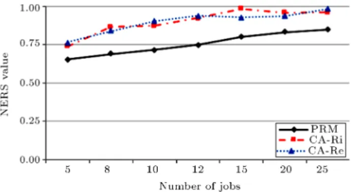
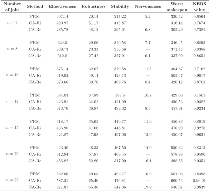
The test problems are simulated in 1000 repeti-tions and the mean value of each dened criterion is calculated for them. The obtained results for PRM, CA-Ri, and CA-Re are shown in Table 6 and Figure 4. Table 6 shows details of computational results ob-tained using PRM, CA-Ri, and CA-Re. These results can be used to evaluate eectiveness and eciency of the proposed solution methods. A general review of the results in Table 6 and Figure 4 shows that:
Figure 4. A comparison between NERS values of dierent solution methods.
Table 6. The mean values of eectiveness and performance criteria according to solution methods. Number
of jobs Method Eectiveness Robustness Stability Nervousness
Worst makespan
NERS value n = 5
PRM 307.14 20.14 214.22 5.2 320.42 0.6564
CA-Ri 290.97 51.17 415.87 | 316.14 0.7674
CA-Re 285.78 48.15 395.01 6.8 305.29 0.7381
n = 8
PRM 324.5 29.06 320.58 7.7 346.45 0.6895
CA-Ri 339.73 23.33 356.56 | 371.45 0.8388
CA-Re 312.8 27.42 357.91 6.1 337.00 0.8651
n = 10
PRM 375.14 32.67 379.58 11.5 404.87 0.7162
CA-Ri 419.02 49.14 423.13 | 505.47 0.9017
CA-Re 370.66 30.76 409.76 8.4 420.12 0.8703
n = 12
PRM 384.03 37.89 388.5 10.7 429.00 0.7501
CA-Ri 423.91 34.02 421.09 | 450.53 0.9382
CA-Re 373.76 36.87 499.32 8.3 457.91 0.9234
n = 15
PRM 418.17 35.65 419.77 11.9 456.86 0.8019
CA-Ri 436.90 41.60 446.81 | 470.90 0.9278
CA-Re 421.87 47.98 497.06 13.9 450.07 0.9631
n = 20
PRM 423.40 46.33 467.50 14.0 550.32 0.8315
CA-Ri 512.94 57.87 469.45 | 578.98 0.9590
CA-Re 456.82 52.80 517.90 16.1 498.55 0.9351
n = 25
PRM 562.06 49.65 499.77 16.5 581.06 0.8498
CA-Ri 587.21 65.40 476.81 | 600.53 0.96.01
CA-Re 571.87 65.36 547.06 19.9 530.07 0.9839
The NERS value of PRM is lower than the NERS
values of the two other methods in each level of jobs. These results show the eciency of the proposed ap-proach compared to two common classical methods;
The NERS value for all solution methods will be
worse when the problem size increases.
With regard to Table 6, the eectiveness of PRM is better than that of other methods for n >= 15. This fact indicates that in addition to NERS, this method also works much better in terms of makespan value of systems with large numbers of jobs.
As mentioned before, the existing coecients in the NERS value measure indicate the importance level of each component. These values are determined by system decision makers such as managers. Changing the values of these coecients will cause change in the proper reaction. To consider the impact of these coecients, we simulated the previous system for 8
dierent levels of coecients for two dierent numbers of jobs (n = 5 and n = 8) to analyze of the inuence of robustness and stability. The values of each component are reported in Tables 7 and 8.
The impact of the stability in the NERS value is considered in Table 7, in which for n = 5 in rows 2 and 3, and ' are xed, and and change; then, in rows 4 and 5, and are xed, and and ' change.
The results show that when the coecient of stability increases and the coecient of nervousness decreases while two other coecients (; ) are xed, the value of stability decreases because its importance increases in the NERS measure. The NERS values in the last column indicate that the coecient of stability has a strong inuence on NERS measure. The same conclusion can be drawn when the coecient of stability increases and the coecient of the robustness decreases while two other coecients (; ') are xed. There are similar conclusions for n = 8.
Table 7. Stability analysis based on dierent coecients of the NERS value components. Number
of jobs ' Eectiveness Robustness Stability Nervousness NERS value
n = 5
0.5 0.3 0.15 0.05 294.89 26.70 161.12 3.5 0.51
0.5 0.3 0.05 0.15 306.85 18.80 219.65 3.9 0.62
0.5 0.05 015 0.3 341.90 57.32 182.29 3.3 0.66
0.5 0.15 0.05 0.3 351.82 53.56 376.01 1.7 0.73
n = 8
0.5 0.3 0.15 0.05 412.90 72.39 229.72 5.9 0.65
0.5 0.3 0.05 0.15 355.90 53.18 210.03 8.2 0.73
0.5 0.05 015 0.3 408.22 87.30 387.12 3.5 0.71
0.5 0.15 0.05 0.3 391.56 80.09 420.76 3.3 0.79
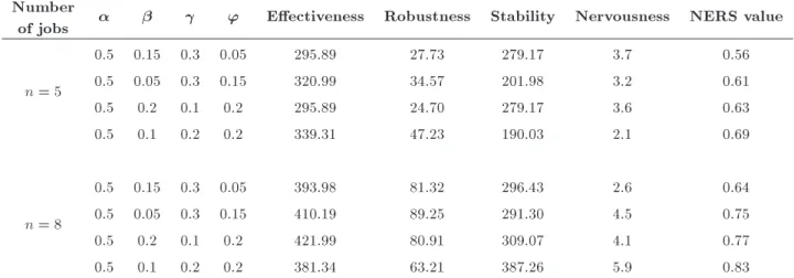
Table 8. Robustness analysis based on dierent coecients of the NERS value components. Number
of jobs ' Eectiveness Robustness Stability Nervousness NERS value
n = 5
0.5 0.15 0.3 0.05 295.89 27.73 279.17 3.7 0.56
0.5 0.05 0.3 0.15 320.99 34.57 201.98 3.2 0.61
0.5 0.2 0.1 0.2 295.89 24.70 279.17 3.6 0.63
0.5 0.1 0.2 0.2 339.31 47.23 190.03 2.1 0.69
n = 8
0.5 0.15 0.3 0.05 393.98 81.32 296.43 2.6 0.64
0.5 0.05 0.3 0.15 410.19 89.25 291.30 4.5 0.75
0.5 0.2 0.1 0.2 421.99 80.91 309.07 4.1 0.77
0.5 0.1 0.2 0.2 381.34 63.21 387.26 5.9 0.83
Table 8 shows the impact of robustness in the NERS value. The results indicate that robustness has a strong inuence on NERS measure, too.
Tables 7 and 8 show that stability is more eective than robustness; thus, a moderate amount is required. Moreover, the tables demonstrate that when and ' are xed and and change, a natural conict between stability and robustness occurs. Based on the results, when increases and decreases, stability and robustness change conversely and this shows the conict between these two measures.
Furthermore, the NERS values for these dierent levels of coecients are considered to gain a proper tradeo between these dierent components and decision makers can choose the best ones based on their opinions.
4.2.1. Comparing eectiveness of solution methods The NERS measure is used to evaluate the performance of the solution methods and to show eectiveness of the proposed method. A single factor ANOVA is used to nd out whether there is a signicant dierence among the performances of solution methods. Data
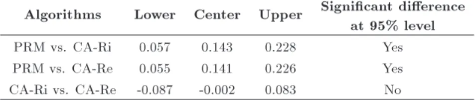
have been made normal and they have equal variances (tested by MINITAB14 software). ANOVA results are presented in Table 9. These results with P-value = 0.003 conrm that there is at least one method with dierent mean response when condence level is set at 0.95. Thus, Fisher's least signicant dierence method is used to compare the performances of methods (see Table 10). The results conrm that there is a signicant dierence between PRM, CA-Ri, and CA-Re. Also, Table 9 shows no signicant dierence between CA-Ri and CA-Re.
As Figure 5 illustrates, among the solution meth-ods, proactive-reactive method for NERS value is better than both the classical approach with right shifting and the classical approach with regeneration.
Table 9. ANOVA results for solution methods.
Source df SS MS F P -value
Algorithm 2 0.09347 0.04674 8.07 0.003 Error 18 0.10426 0.00579
Table 10. Fisher 95% individual condence intervals for all pair-wise comparisons. Algorithms Lower Center Upper Signicant dierence
at 95% level
PRM vs. CA-Ri 0.057 0.143 0.228 Yes
PRM vs. CA-Re 0.055 0.141 0.226 Yes
CA-Ri vs. CA-Re -0.087 -0.002 0.083 No
Figure 5. Means and interval plot for NERS value.
Therefore, the superiority of the proposed solution approach is concluded over other heuristics including CA-Ri and CA-Re due to the computational results. 5. Conclusions
In this paper, a proactive-reactive approach was
pre-sented instead of SMs. This two-stage approach
produced robust and stable solutions for a two-machine scheduling problem in a ow shop environment. In this approach, rstly, by considering uncertain processing times and using the robust optimization approach, the problem was solved and a robust initial solution was proactively produced. Then, in case of machine failure, the appropriate reaction was adopted based on the dened performance measure. This measure was a multi-criteria measure dened in terms of solution eectiveness, robustness, stability, and reduction of system nervousness. Computational results indicated that this method was much more eective than the ordinary scheduling methods that operated on the basis of makespan alone. The results showed eciency of the proposed approach compared to two common classical methods in the face of unexpected failures. For future research, this problem can be considered for other scheduling problems of shop oor, and other classical objectives can be used to evaluate this method. As another research subject, random distributions can be considered for the occurrence time of failure and repair duration, because they can be used for obtaining initial solutions that are proactively able to reduce the eect of machine breakdown. Moreover, the eect of this approach on other random disruptions such as the arrival of new jobs, order cancellations, etc. can be
investigated and analyzed. Another important future research could be the presentation of proper heuristic methods for machine failure, which can be applied in the second step of this approach.
References
1. Beck, J.C. \Solution-guided multi-point constructive search for job shop scheduling", J. Artif. Intell. Res., 29, pp. 49-77 (2007).
2. Beck, J.C. and Wilson, N. \Proactive algorithms for job shop scheduling with probabilistic durations", J. Artif. Intell. Res., 28, pp. 183-232 (2007).
3. Sabuncuoglu, I. and Goren, S. \Hedging production schedules against uncertainty in manufacturing en-vironment with a review of robustness and stability research", Int. J. Comput. Integr. Manuf., 22(2), pp. 138-157 (2009).
4. Ouelhadj, D. and Petrovic, S. \A survey of dynamic scheduling in manufacturing systems", J. Scheduling., 12, pp. 417-43 (2009).
5. Kuchta, D. \A concept of a robust solution of a multi criteria linear programming problem", Cent. Eur. J. Oper. Res., 19, pp. 605-613 (2011).
6. O'Donovan, R., Uzsoy, R. and McKay, K.N. \Pre-dictable scheduling of a single machine with break-downs and sensitive jobs", Int. J. Prod. Res., 37(18), pp. 4217-4233 (1999).
7. Pinedo, M.L., Scheduling: Theory, Algorithms, and Systems, Springer, 3rd Edition (2008).
8. Fattahi, P., Hosseini S.M.H. and Jolai, F. \A math-ematical model and extension algorithm for assembly exible ow shop scheduling problem", Int. J. Adv. Manuf., 65(5-8), pp. 787-802 (2012).
9. Daniels, R. and Kouvelis, P. \Robust scheduling to hedge against processing time uncertainty in single stage production", Manag. Sci., 41(2), pp. 363-376 (1995).
10. Kouvelis, P., Kurawarwala, A.A. and Gutierrez, G.J. \Algorithms for robust single- and multiple-period layout planning for manufacturing systems", Eur. J. Oper. Res., 63, pp. 287-303 (1992).
11. Mulvey, J.M., Vanderbei, R.J. and Zenios, S.A. \Ro-bust optimization of large-scale systems", Oper. Res., 43, pp. 264-281 (1995).
12. Rossi, A. \A robustness measure of the conguration of multi-purpose machines", Int. J. Prod. Res., 48(4), pp. 1013-1033 (2010).
13. Kutanoglu, E. and Sabuncuoglu, I. \Experimental investigation of iterative simulation-based scheduling in a dynamic and stochastic job shop", J. Manuf. Syst., 20(4), pp. 264-279 (2001).
14. Wu, S.D., Storer, R.N. and Chang, P. \One-machine rescheduling heuristics with eciency and stability as criteria", Comput. Oper. Res., 20(1), pp. 1-14 (1993). 15. Leon, V.J., Wu, S.D. and Storer, R.H. \Robustness measures and robust scheduling for job shops", IIE. Trans., 26(5), pp. 32-43 (1994).
16. Lawrence, S.R. and Sewell, E.C. \Heuristic, optimal, static, and dynamic schedules when processing times are uncertain", J. Oper. Manag., 15, pp. 71-82 (1997). 17. Sabuncuoglu, I. and Karabuk, S. \Rescheduling fre-quency in an FMS with uncertain processing times and unreliable machines", J. Manufacturing., 18(4), pp. 268-283 (1999).
18. Jensen, M.T. \Generating robust and exible job shop schedules using genetic algorithms", IEEE. Trans. Evolut. Comput., 7(3), pp. 275-288 (2003).
19. Goren, S. and Sabuncuoglu, I. \Robustness and stabil-ity measures for scheduling: single machine environ-ment", IIE. Trans., 40(1), pp. 66-83 (2008).
20. Sotskov, Y.N., Egorova, N.G. and Lai, T.C. \Mini-mizing total weighted ow time of a set of jobs with interval processing times", Math. Comput. Model., 50, pp. 556-73 (2009).
21. Bouyahia, Z., Bellalouna, M., Jaillet, P. and Ghedira, K. \A priori parallel machines scheduling", Comput. Ind. Eng., 58(3), pp. 488-500 (2010).
22. Ghezail, F., Pierreval, H. and Hajri-Gabouj, S. \Anal-ysis of robustness in proactive scheduling: A graphi-cal approach", Comput. Oper. Res., 58, pp. 193-198 (2010).
23. Al-Hinai, N. and ElMekkawy, T.Y. \Robust and stable exible job shop scheduling with random machine
breakdowns using a hybrid genetic algorithm", Int. J. Prod. Econ., 132, pp. 279-291 (2011).
24. Al-Hinai, N. and ElMekkawy, T.Y. \An ecient hy-bridized genetic algorithm architecture for the exible job shop scheduling problem", Flex. Serv. Manuf. J., 23, pp. 64-85 (2011).
25. Leung, S.C.H. and Wu, Y. \A robust optimization model for stochastic aggregate production planning", Prod. Plan. Control., 15(5), pp. 502-514 (2004). 26. YU, C.S. and LI, H.L. \A robust optimization model
for stochastic logistic problems", Int. J. Prod. Econ., 64, pp. 385-397 (2000).
27. Gan, H.S. and Wirth, A. \Comparing deterministic, robust and online scheduling using entropy", Int. J. Prod. Res., 43(10), pp. 2113-2134 (2005).
28. Rahmani, D. and Heydari, M. \Robust and stable ow shop scheduling with unexpected arrivals of new jobs and uncertain processing times", J. Manuf. Syst., 33(1), pp. 84-92 (2014).
29. Hwang, C.L. and Yoon, K., Multiple Attribute Decision Making: Methods and Applications, Springer-Verlag, Berlin (1981).
Biography
Donya Rahmani is an Assistant Professor of In-dustrial Engineering at K. N. Toosi University of Technology. She received her BSc degree in Industrial Engineering from Bu-Ali Sina University and MSc and PhD degrees both in Industrial Engineering from Iran University of Science and Technology. Her research in-terests are in production planning, robust optimization, dynamic scheduling, and operations research. She is a reviewer of several international journals.