ISSN 2307-7743 http://scienceasia.asia
_______________
2010 Mathematics Subject Classification: 65L06.
Key words and phrases: Sixth order R-K method, Second order ODEs, Transformation, New coefficient Tableau, A-stable, Low implementation cost, Error formula
© 2015 Science Asia 1 / 10
AN IMPLICIT RUNGE-KUTTA METHOD FOR GENERAL SECOND ORDER ORDINARY DIFFERENTIAL EQUATIONS
SA AGAM, YA YAHAYA AND SC OSUALA
Abstract. This paper focuses on the derivation of a fully implicit Sixth order Runge-kutta type method with error estimation formula for the solution of general second order ordinary differential equations (ODEs). We define a transformation on the set of coefficients (Butcher coefficients Tableau) for first order differential equations to generate a new coefficient tableau for direct solution of second order ODEs. The scheme is simple, A-stable, highly efficient and has low implementation cost. Some problems are used as experimental examples.
1.0 Introduction
Development of Runge-kutta method for direct solution of second order Odes started with Nystrom [1]. He extended the fourth order explicit Runge-kutta method for first order ODEs to second order differential equations. Earlier researchers include Huta [2], Felhberg [3], Chawla et al [4], Sharp et al [5], Imoni et al [6] Coper et al [7], Filippi et al[8], Hairer [9] and Agam et al [10] etc. All these methods mentioned above are explicit type. Explicit Runge-kutta methods are unsuitable for solution of Stiff problems because their region of absolute stability is small, in particular they are bounded.
The instability of explicit methods motivates the development of implicit methods. Implicit Runge-kutta methods were earlier proposed by Kuntzmann [11] and Butcher [12]. Their proposed methods are based on Gauss quadrature. The remarkable thing about these methods are that their order 𝑝 = 2𝑠, for an S-stage scheme and are all A-stable [13]
The Gauss-quadrature method is a generalization of integrals in the interval (-1,1). The Gauss-quadrature methods mentioned above are for first order differential equations. Thus there is need to develop parallel Runge-kutta methods for second and higher orders ODEs. In this paper we have tried to address these problems by deriving Runge-kutta method based on Gauss-quadrature for second order ODEs.
1.1 Preliminaries/ Basic definition
1.2 Definition: Let 〈𝐺1∗〉 and 〈𝐺2 . 〉 be two set 𝐺1 and 𝐺2 with binary operations (∗) and (. ) respectively. A transformation 𝑇: 𝐺1 → 𝐺2 is a linear monomorphism if for any two
𝑇(𝑎1∗ 𝑎2) = 𝑇(𝑎1) . 𝑇(𝑎2) and 𝑇(𝑎1) = 𝑇(𝑎2) ⇒ 𝑎1 = 𝑎2
Remark: A monomorphism operators preserve the algebraic structure of the domain into its co domain.
1.2 A Butcher Tableau of coefficients based on Gauss Lengendre quadrature [14] of order 6, for solving first order ordinary differential equation is given below
Table1 Butcher Coefficients table of order 6 for first order differential equations
𝐶 A
(1 2−
√15 10)
5
36 (
2 9−
√15
15) (
5 36−
√15 30) 1
2 (
5 36+
√15
24)
2
9 (
5 36−
√15 24) (1
2+ √15
10) (
5 36+
√15
30) ( 2 9+
√15 15)
5 36 𝑏𝑇
5
18 4 9
5 18
C A
𝑏𝑇 (𝑏1, 𝑏2, … . 𝑏𝑠)
where 𝐴 = (𝑎𝑖𝑗) 𝐶 = (𝑐1, 𝑐2, … . 𝑐𝑠)
𝑏𝑇 = (𝑏1, 𝑏2, … . , 𝑏𝑠) (1.0) 1.4 Error of a Runge-kutta method is defined as
𝑦(𝑥𝑖) − 𝑦𝑖 = (Exact error)
Where 𝑦(𝑥𝑖) is the exact solution at 𝑥 = 𝑥𝑖 and 𝑦𝑖 is the RK solution at 𝑥 = 𝑥𝑖.
2.0 Derivation method
We consider the general second order ODEs 𝑎2𝑦′′+ 𝑎
1𝑦′+ 𝑎0𝑦 = 𝑔(𝑥, 𝑦), 𝑦′(𝑥0) = 𝑦′0 (2.01)
where 𝑎𝑖𝑖 = 0,1,2 are scalar constants or functions. We then rewrite 2.01 in the form
𝑦′′ = 𝑓(𝑥, 𝑦, 𝑦′), 𝑦(𝑥
0) = 𝑦0, 𝑦′(𝑥0) = 𝑦′0 (2.02)
= 𝑓(𝑣), 𝑣 = (𝑥, 𝑦, 𝑦′)
We use the coefficient tableau (1.0) ∈ ℝ3as our basis and domain of transformation T
defined as follows.
𝑣𝑖 = (𝑥 + 𝑐𝑖ℎ , 𝑦 + ∑ 𝑎𝑖𝑗𝑇(𝑣𝑗), 𝑦′ +
3
𝑗=1
∑ 𝑎𝑖𝑗𝑇′(𝑣𝑗)
3
𝑗=1
𝑇(𝑣𝑖) = 𝑇 (𝑥 + 𝑐𝑖ℎ , 𝑦 + ∑ 𝑎𝑖𝑗𝑇(𝑣𝑗), 𝑦′ +
3
𝑗=1
∑ 𝑎𝑖𝑗𝑇′(𝑣𝑗)
3
𝑗=1
) = ℎ (𝑦′+ ∑ 𝑎
𝑖𝑗𝑇′(𝑣𝑗) 3
𝑗=1
)
and
𝑇′(𝑣𝑖) = ℎ𝑓 (𝑥 + 𝑐𝑖ℎ , 𝑦 + ∑ 𝑎𝑖𝑗𝑇(𝑣𝑗), 𝑦′ +
3
𝑗=1
∑ 𝑎𝑖𝑗𝑇′(𝑣𝑗)
3
𝑗=1
) = ℎ 𝑚𝑖
i. e. 𝑚𝑖 = 𝑓 (𝑥 + 𝑐𝑖ℎ , 𝑦 + ∑ 𝑎𝑖𝑗𝑇(𝑣𝑗), 𝑦′ +
3
𝑗=1
∑ 𝑎𝑖𝑗𝑇′(𝑣𝑗)
3
𝑗=1
) (2.03)
Theorem 1
The Transformation 𝑇: ℝ3 ⟶ ℝ in (2.03) is a well defined monomorphism.
Proof:
let 𝑢, 𝑣 ∈ ℝ defined by
𝑈 = (𝑥 + 𝑐𝑖ℎ , 𝑦1+ ∑ 𝑎𝑖𝑗𝑇(𝑢𝑗), 𝑦′1 +
3
𝑗=1
∑ 𝑎𝑖𝑗𝑇′(𝑢𝑗)
3
𝑗=1
)
𝑉 = (𝑥 + 𝑐𝑖ℎ , 𝑦2+ ∑ 𝑎𝑖𝑗𝑇(𝑣𝑗), 𝑦′2+
3
𝑗=1
∑ 𝑎𝑖𝑗𝑇′(𝑣𝑗)
3
𝑗=1
)
by the definition of T on ℝ3 ,we have
𝑇(𝑈 + 𝑉) = ℎ ( 𝑦′
1 + ∑ 𝑎𝑖𝑗𝑇′(𝑢𝑗) 3
𝑗=1
+ 𝑦′
2+ ∑ 𝑎𝑖𝑗𝑇′(𝑣𝑗) 3
𝑗=1
)
= ℎ ( 𝑦′
1+ ∑ 𝑎𝑖𝑗𝑇′(𝑢𝑗) 3
𝑗=1
) + ℎ ( 𝑦′
2 + ∑ 𝑎𝑖𝑗𝑇′(𝑣𝑗) 3
𝑗=1
)
= 𝑇(𝑈) + 𝑇(𝑉)
Hence T is a homomorphism. Now we show that T is one to one
Let 𝑢, 𝑣 ∈ ℝ3 ,with 𝑇(𝑢) = 𝑇(𝑣), then by definition of T, we have
ℎ ( 𝑦1+ ∑ 𝑎𝑖𝑗𝑇′(𝑢𝑗)
3
𝑗=1
) = ℎ ( 𝑦2+ ∑ 𝑎𝑖𝑗𝑇′(𝑣𝑗)
3
𝑗=1
)
Since 𝑇(𝑢) = 𝑇(𝑣) then 𝑇′(𝑢
𝑗) = 𝑇′(𝑣𝑗) (2.04)
Hence 𝑦1 = 𝑦2 and so
(𝑥 + 𝑐𝑖ℎ , 𝑦1+ ∑ 𝑎𝑖𝑗𝑇(𝑢𝑗), 𝑦′1+
3
𝑗=1
∑ 𝑎𝑖𝑗𝑇′(𝑢𝑗)
3
𝑗=1
) = (𝑥 + 𝑐𝑖ℎ , 𝑦2+ ∑ 𝑎𝑖𝑗𝑇(𝑣𝑗), 𝑦′2+
3
𝑗=1
∑ 𝑎𝑖𝑗𝑇′(𝑣𝑗)
3
𝑗=1
Hence 𝑈 = 𝑉
Thus T is one to one ⇒ monomorphism
Remark: By implication the domain of T and the image of T have the same algebraic structure.
We now use this transformation to generate new coefficients and Butcher tableau for direct solution of (2.02).
Using this transformation we have
𝑇(𝑣1) = ℎ ( 𝑦′ + ∑ 𝑎1𝑗𝑇(𝑣𝑗)
3
𝑗=1
) = ℎ ( 𝑦′ + ∑ 𝑎1𝑗 ℎ𝑚𝑗 3
𝑗=1
)
= ℎ(𝑦′+ 𝑎11ℎ𝑚1+ 𝑎12ℎ𝑚2+ 𝑎13ℎ𝑚3) , where (𝑎𝑖𝑗 ∈ 𝑇𝑎𝑏𝑙𝑒 1)
= ℎ ( 𝑦′+ 5
36ℎ𝑚1+ ( 2 9−
√15
15 ) ℎ𝑚2+ ( 5 36−
√15
30 ) ℎ𝑚3) Similarly,
𝑇(𝑣2) = 𝑇 (𝑥 + 𝑐2ℎ , 𝑦 + ∑ 𝑎2𝑗𝑇(𝑣𝑗), 𝑦′+ 3
𝑗=1
∑ 𝑎2𝑗𝑇′(𝑣𝑗)
3
𝑗=1
)
= ℎ( 𝑦′+ 𝑎21ℎ𝑚1+ 𝑎22ℎ𝑚2+ 𝑎23ℎ𝑚3)
= ℎ ( 𝑦′+ (5
36+ √15
24 ) ℎ𝑚1+ 2
9ℎ𝑚2+ ( 5 36−
√15
24 ) ℎ𝑚3) 𝑇(𝑣3) = ℎ(𝑦′+ 𝑎
31𝑇′(𝑣1) + 𝑎32𝑇′(𝑣2) + 𝑎33𝑇′(𝑣3))
= ℎ (𝑦′+ (5
36+ √15
30 ) ℎ𝑚1+ ( 2 9+
√15
15 ) ℎ𝑚2+ 5
36ℎ𝑚3) By the definition of T, from (2.03)
𝑚𝑖 = 𝑇′(𝑉
𝑗) = 𝑓 (𝑥 + 𝑐𝑖ℎ , 𝑦 + ∑ 𝑎𝑖𝑗𝑇(𝑣𝑗), 𝑦′+ 3
𝑗=1
∑ 𝑎𝑖𝑗𝑇′(𝑣𝑗)
3
𝑗=1
)
Now substituting for 𝑇(𝑉𝑖) from (2.03 ), we have
𝑚1 = (𝑓𝑥 + 𝑐1ℎ, 𝑦 + 𝑎11𝑇(𝑣1) + 𝑎12𝑇(𝑣2) + 𝑎13𝑇(𝑣3), 𝑦′+ 𝑎
11𝑇′(𝑣1) + 𝑎12𝑇′(𝑣2)
+ 𝑎13𝑇′(𝑣3))
𝑚1 = 𝑓 (𝑥 + (1 2−
√15
10 ) ℎ , 𝑦 + 5
36ℎ (𝑦′ + ∑ 𝑎𝑖𝑗𝑇(𝑣𝑗)
3
𝑗=1
) + (2 9−
√15
15 ) ℎ (𝑦′ + ∑ 𝑎𝑖𝑗𝑇(𝑣𝑗)
3
𝑗=1
)
+ (5 36−
√15
30) ℎ (𝑦′ + ∑ 𝑎𝑖𝑗𝑇(𝑣𝑗)
3
𝑗=1
) , 𝑦′+ 5
36ℎ𝑚1+ ( 2 9−
√15
15 ) ℎ𝑚2+ ( 5 36−
√15
30 ) ℎ𝑚3),
(𝑇′(𝑣
𝑖) = ℎ𝑚𝑖)
𝑚1 = 𝑓 (𝑥 + (1 2−
√15
10 ) ℎ, 𝑦 + ( 1 2−
√15 10 ) ℎ𝑦
′+ 1
90ℎ
2𝑚
1+ (
7 90−
√15 45 ) ℎ
2𝑚
2
+ (1 9−
√15 36 ) ℎ
2𝑚
3 , 𝑦′+
5
36ℎ𝑚1+ ( 2 9−
√15
15 ) ℎ𝑚2+ ( 5 36−
√15
30 ) ℎ𝑚3) similarly
𝑚2 = 𝑓 [𝑥 +1
2ℎ , 𝑦 + 𝑎21𝑇(𝑣1) + 𝑎22𝑇(𝑣2) + 𝑎23𝑇(𝑣3), 𝑦
′+ 𝑎
21𝑇′(𝑣1) + 𝑎22𝑇′(𝑣2)
+𝑎23𝑇′(𝑣3)]
= 𝑓 (𝑥 +1
2ℎ, 𝑦 + ( 5 36+
√15
24 ) ℎ (𝑦′ + ∑ 𝑎1𝑗ℎ𝑚𝑗
3
𝑗=1
) +2
9ℎ (𝑦′ + ∑ 𝑎2𝑗ℎ𝑚𝑗
3
𝑗=1
)
+ (5 36−
√15
24 ) ℎ (𝑦′ + ∑ 𝑎3𝑗ℎ𝑚𝑗
3
𝑗=1
) , 𝑦′+ 𝑎21ℎ𝑚1+ 𝑎22ℎ𝑚2+ 𝑎23ℎ𝑚3)
𝑚2 = 𝑓 (𝑥 +1 2ℎ, 𝑦 +
1 2ℎ𝑦
′+ ( 7
144+ √15
72 ) ℎ
2𝑚
1+
1 36ℎ
2𝑚
2+ (
7 144−
√15 72 ) ℎ
2𝑚
3,
𝑦′+ (5
36+ √15
24 ) ℎ𝑚1+ 2
9ℎ𝑚2 + ( 5 36−
√15
24 ) ℎ𝑚3)
𝑚3 = 𝑓 (𝑥 + (1 2+
√15
10) ℎ , 𝑦 + 𝑎31𝑇(𝑣1) + 𝑎32𝑇(𝑣2) + 𝑎33𝑇(𝑣3) , 𝑦
′+ 𝑎
31𝑇′(𝑣1) + 𝑎32
+𝑎32𝑇′(𝑣2) + 𝑎33𝑇′(𝑣3))
= 𝑓 (𝑥 + (1 2+
√15
10 ) ℎ, 𝑦 + 𝑎31ℎ (𝑦′ + ∑ 𝑎1𝑗ℎ𝑚𝑗
3
𝑗=1
) + 𝑎32ℎ (𝑦′ + ∑ 𝑎2𝑗ℎ𝑚𝑗 3
𝑗=1
)
+𝑎33ℎ (𝑦′ + ∑ 𝑎3𝑗ℎ𝑚𝑗
3
𝑗=1
) , 𝑦′+ ∑ 𝑎
3𝑗ℎ𝑚𝑗
3
𝑗=1
)
Substituting for 𝑎𝑖𝑗 from table 1 and simplify, we have
𝑚3 = 𝑓 (𝑥 + (1 2+
√15
10) ℎ, 𝑦 + ( 1 2+
√15 10 ) ℎ𝑦
′+ (1
9+ √15
36 ) ℎ
2𝑚
1+ (
7 90+
√15 45) ℎ
2𝑚
2
+ 1 90ℎ
2𝑚
3, 𝑦′+ (
5 36+
√15
30 ) ℎ𝑚1+ ( 2 9+
√15
15 ) ℎ𝑚2+ 5
36ℎ𝑚3) The general solution of (2.02) is define as
𝑦𝑛+1 = 𝑦𝑛+ 𝑏1𝑇(𝑣1) + 𝑏2𝑇(𝑣2) + 𝑏3𝑇(𝑣3)
𝑦𝑛+ 5
18ℎ (𝑦
′+ 5
36ℎ𝑚1+ (
2
9+
√15
15) ℎ𝑚2+ (
5
36−
√15
30) ℎ𝑚3) +
4
9ℎ (𝑦
′+ (5
36+
√15
24) ℎ𝑚1+
2
9ℎ𝑚2+ (
5
36−
√15
24) ℎ𝑚3) + 5
18ℎ (𝑦
′+ (5
36+
√15
30) ℎ𝑚1+ (
2
9+
√15
15) ℎ𝑚2+
5
(2.05) 𝑦′𝑛+1= 𝑦′𝑛+ 𝑏1𝑇′(𝑣1) + 𝑏2𝑇′(𝑣2) + 𝑏3𝑇′(𝑣3)
= 𝑦′𝑛+ 5
18ℎ𝑚1+ 8
18ℎ𝑚2+ 5 18ℎ𝑚3
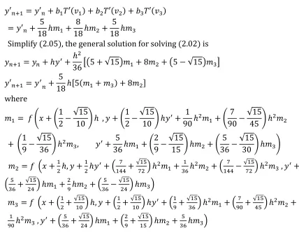
Simplify (2.05), the general solution for solving (2.02) is
𝑦𝑛+1 = 𝑦𝑛+ ℎ𝑦′+ ℎ 2
36[(5 + √15)𝑚1+ 8𝑚2+ (5 − √15)𝑚3]
𝑦′𝑛+1= 𝑦′
𝑛+
5
18ℎ[5(𝑚1 + 𝑚3) + 8𝑚2]
where
𝑚1 = 𝑓 (𝑥 + (
1 2−
√15
10 ) ℎ , 𝑦 + ( 1 2−
√15 10) ℎ𝑦
′+ 1
90ℎ
2𝑚
1+ (
7 90−
√15 45 ) ℎ
2𝑚
2
+ (1 9−
√15 36) ℎ
2𝑚
3, 𝑦′+
5
36ℎ𝑚1+ ( 2 9−
√15
15 ) ℎ𝑚2+ ( 5 36−
√15
30 ) ℎ𝑚3)
𝑚2 = 𝑓 (𝑥 +1
2ℎ, 𝑦 + 1
2ℎ𝑦
′+ ( 7
144+
√15
72) ℎ
2𝑚
1+
1
36ℎ
2𝑚
2+ (
7
144−
√15
72) ℎ
2𝑚
3 , 𝑦′+
(5
36+
√15
24) ℎ𝑚1+
2
9ℎ𝑚2+ (
5
36−
√15
24) ℎ𝑚3)
𝑚3 = 𝑓 (𝑥 + (1
2+
√15
10) ℎ, 𝑦 + ( 1
2+
√15
10) ℎ𝑦
′+ (1
9+
√15
36) ℎ
2𝑚
1+ (
7
90+
√15
45) ℎ
2𝑚
2 +
1 90ℎ
2𝑚
3 , 𝑦′+ ( 5
36+
√15
24) ℎ𝑚1+ (
2
9+
√15
15) ℎ𝑚2 +
5
36ℎ𝑚3)
3.0 Analysis of the scheme
The method for the second order ODEs is summarized in table 2: Table 2: Butcher’s tableau for second order ODEs
𝐶 𝐴 𝐴′
(1 2− √15 10) 5 36 ( 2 9− √15 15) (
5 36− √15 30) 1 90 ( 7 90− √15 45) (
1 9− √15 36) 1 2 ( 5 36+ √15 24) 2 9 ( 5 36− √15 24) (
7 144+ √15 72) 1 36 ( 7 144− √15 72) (1 2+ √15
10) ( 5 36+
√15 30) (
2 9+ √15 15) 5 36 ( 1 9+ √15 36) (
7 90+ √15 45) 1 90
1 5
18 8 18 5 18 1
36(5 + √15)
8 36
1
36(5 − √15)
𝑏𝑇 𝑏′𝑇
= 𝐶 𝐴𝑋𝐴′ = 𝑅(𝑇) ∈ ℜ3
Consistency: Table 1since the (Domain of T) is consistent, we concluded that table 2, is also consistent because it is the range of T. Since the Dim(T) is isomorphic to Rang(T) and T preserve the algebraic structure of Domain onto Rang(T )
Stability: The test stability equation is 𝑦′′ = 𝜆𝑦, 𝜆 < 0
For stability region, we set 𝑍 = 𝜆ℎ2
The stability function is defined as 𝑅(𝑧) where 𝑅(𝑧) = 𝐼 + (𝑍𝑏𝑇+ 𝑍2𝑏′𝑇) (𝐼𝑍𝐴 − 𝑍2𝐴′)−1𝑒
𝑒 = (1,1,1)𝑇, ℎ 𝜖 (0,1), D = 𝐴 x 𝐴′ is the coefficient matrix, I is the identity 3 x 3 matrix, 𝑍 = 𝜆ℎ2, 𝐵 = (𝑏
1, 𝑏2, 𝑏3), 𝑏′= (𝑏′1, 𝑏′2, 𝑏′3) weights.
The A-stability Region is
(𝑅(𝑧)) = {𝑧: 𝑅(𝑧) < 0 𝑎𝑛𝑑 |𝑅(𝑧)| ≤ 1}
Our method is automatically A-stable since the Dim(T) based on Gauss quadrature method which is A-stable (see Butcher [4]), and T preserve its algebraic structure onto its Range. Error: Since every Runge-kutta solution agree with Taylor’s series expansion of order 𝑝 = 6
The error is 𝐶(ℎ𝑝+1) = 𝐶(ℎ7)
Proposition 1 (Error estimation formula)
If 𝑦𝑛+1(ℎ) 𝑎𝑛𝑑 𝑦𝑛+1(
ℎ
2) are approximate solutions of a Runge-kutta type method of order P with
step size ℎ 𝑎𝑛𝑑ℎ
2 respectively, then the error 𝐶(ℎ
𝑝+1) is
𝐸𝑟 = 2
𝑝+1
2𝑝+1− 1[𝑦𝑛+1 (ℎ2)
− 𝑦𝑛+1(ℎ)]
Proof
Let 𝑦𝑛+1(ℎ) and 𝑦𝑛+1(
ℎ
2) be approximation solution of Runge-kutta method of order p respectively.
These solutions can be expanded into Taylor’s series and Runge-kutta solutions agrees with the Taylor’s series expansion up to the p terms and converges to exact solution 𝑦𝑛+1 .Thus we can write
𝑦𝑛+1= 𝑦𝑛+1 (ℎ)
+ 𝐶(ℎ𝑝+1) + 𝑅𝑛(𝑥) … … (𝑖) (2.06 )
𝑦𝑛+1= 𝑦𝑛+1(
ℎ
2) + 𝐶 (ℎ
2)
𝑝+1
+ 𝑄𝑛(𝑥) … … (𝑖𝑖) (2.07)
𝑎𝑠 𝑝 → ∞, 𝑅𝑛(𝑥)& 𝑄𝑛(𝑥) → 0, hence 𝑅𝑛(𝑥) & 𝑄𝑛(𝑥) can be ignored. Then subtracting
(2.07) from (2.06) we have
0 = 𝑦𝑛+1(ℎ) − 𝑦𝑛+1(
ℎ
2) + 𝐶(ℎ𝑝+1) (2𝑝+1− 1
𝐶(ℎ𝑝+1) = 2 𝑝+1
2𝑝+1− 1(𝑦𝑛+1 (ℎ2)
− 𝑦𝑛+1(ℎ))
Since 𝐶(ℎ𝑝+1) is the first neglect term of the series, our truncated error is 𝐶(ℎ𝑝+1). Thus
our error is
𝐶(ℎ𝑝+1) = 𝐸
𝑟 =
2𝑝+1
2𝑝+1−1(𝑦𝑛+1 (ℎ2)
− 𝑦𝑛+1(ℎ))
Remark: Since our method is of order 6. The error of our Runge-kutta method is
𝐸𝑟 =
27
27− 1(𝑦𝑛+1 (ℎ2)
− 𝑦𝑛+1(ℎ)) (error estimation formula) (2.08)
4.0Numerical Experiments
In this section we test the performances of our schemes by considering some problems with exact solutions to check quality, stability and implementation cost of our schemes
Example 1
𝑦′′ = 𝑥(𝑦′)2, 𝑦(0) = 1, 𝑦′(0) =1 2 Analytic solution: 𝑦(𝑥) = 1 +1
2𝐼𝑛 (
2+𝑥 2−𝑥)
Example 2
𝑦′′− 3𝑦′+ 2𝑦 = 𝑥 , 𝑦(0) = 1, 𝑦′(0) = 0 Analytic solution: 𝑦(𝑥) = 𝑒𝑥−3
4𝑒
2𝑥+1
2𝑥 +
3 4
Example 3
𝑦′′ = −100𝑦, 𝑦(0) = 1, 𝑦′(0) = 10 , ℎ = 0.01
Analytic solution: 𝑦(𝑥) = 𝐶𝑜𝑠 (10 𝑥) + 𝑆𝑖𝑛 (10 𝑥)
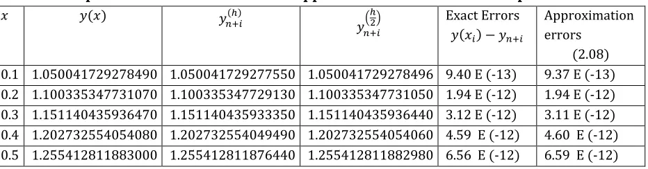
Table 3: Comparison of the theoretical and approximate solutions for example 1
𝑥 𝑦(𝑥) 𝑦
𝑛+𝑖 (ℎ)
𝑦𝑛+𝑖(
ℎ
2) Exact Errors
𝑦(𝑥𝑖) − 𝑦𝑛+𝑖
Approximation errors
Table 4: Comparison of the theoretical and approximate solutions for example 2
𝑥 𝑦(𝑥) 𝑦
𝑛+𝑖 (ℎ)
𝑦𝑛+𝑖(
ℎ
2) Exact Errors
𝑦(𝑥𝑖) − 𝑦𝑛+𝑖
Approximation errors
(2.08) 0.1 0.989118849455522 0.989118849340112 0.989118849453719 1.15 E (-10) 1.15 E (-10) 0.2 0.952534234929220 0.952534234647043 0.952534234924814 2.82 E (-10) 2.80 E (-10) 0.3 0.883269707283120 0.883269706765726 0.883269707275048 5.17 E (-10) 5.13 E (-10) 0.4 0.772669001271920 0.772669000428699 0.772669001258759 8.43 E (-10) 8.37 E (-10) 0.5 0.610009899355840 0.610009898067594 0.610009899335757 1.29 E (-09) 1.28 E (-09)
Table 5: Comparison of the theoretical and approximate solutions for example 3
𝑥 𝑦(𝑥) 𝑦
𝑛+𝑖
(ℎ) Error [15] Exact Error
0.01 1.094837581924850 1.094837581923960 1.0 E (-08) 8.90E (-13) 0.02 1.178735908636300 1.178735908363475 2.3 E (-08) 1.55 E (-12) 0.03 1.250856695786950 1.25085669578490 4.0E (-08) 1.98 E (-12) 0.04 1.310479336311540 1.310479336309410 5.1 E (-08) 2.13 E (-12) 0.05 1.357008100494580 1.357008100492580 6.9 E (-08) 2.00E (-12)
5.0 Discussion of Results
We observed from the three problems tested the approximate error method (2.08) converges to the exact errors. This shows that our method is good and can be used to solve accurately problems without exact solutions. (see tables 3,4 and 5). The new method has only three function evaluations 𝑚1, 𝑚2, 𝑚3 which are directly used for integration of the problems. The method is much better than that of [15] (see table 5) in terms of accuracy and implementation cost.
6.0 Conclusion
We have used three Gauss-quadrature points to derived a 6th order implicit Runge-kutta
method for direct integration of second order differential equations. The method is A-stable, highly efficient and has simple coefficients with low implementation cost. Alongside we develop an accurate error formula for step size control.
Competing of Interests
REFERENCES
[1] Nystrom EJ (1925) Uber die Numerische integration von differential gleichungen, Acta soc. Fennice, 50(13) 55
[2] Huta A (1965) Une amelioration de method de Runge-kutta Nystrom pour la resolution numenique des equation differentielles du premier, Acta math, uni. Comenian P21-24
[3] Felhberg E (1972) Classical eight and lower order Nystrom formulae with step size control for special second order ODEs. Nasa Tech report R-381, Summary, Computing 10, p305-315
[4] Chawla MM and Sherma SR (1981) Intervals of periodicity and absolute stability of explicit Nystrom method for y′′= f(x, y), BIT, volume 21, pages 455-464
[5] Sharp PW and Fine JM (1992) Some Nystron pairs for the general second order initial value problems. Journal of Computational and applied mathematics, volume 42, pages 279- 291
[6] Imoni So, Otunta FO and Ramanohan TR (2006) Embedded Implicit Runge-kutta Nystrom method for solving second order ODEs. International Journal of Computer Mathematics, volume 83, No11 pages 777-784
[7] Cooper GJ and Verner JH (1972) Some explicit Runge-kutta methods of high order. SIAM Journal of Numerical Analysis, volume 9, pages 389-405
[8] Fillip S and Graf S (1986) new Runge-kutta Nystrom formula pair Order 8(7), 9(8), 10(9) and 11(10) for ODEs of the form y′′= f(x, y). Journal of computational and Applied mathematics, volume14 pages
361-370
[9] Hairer E (1977) Methodes de Nystrom pour L’equation differentiable y′′= f(x, y) , Numerical
Mathematics, volume 27,pages 283-300
[10] Agam SA and Ekpeyong FE (2013) Upgrading Runge-kutta-Felhberg method for second order ODEs. International Journal of Science and Technology, volume 3, Number 4 pages 244-249
[11] Kuntzmann J (1961) Neure entwickhingen der methoden von Runge and Kutta, Z Angew Math Mech. 4`1 T28-T31
[12] Butcher J C (1964) Implicit Runge-kutta process, Journal of Mathematics computer volume 18 pages 50-64 [13] Butcher J C (1996) A history of Runge-kutta methods. Journal of Applied Numerical Mathematics.
Volume 20 pp247-260
[14] Press WH, Flannery, Brain P, TTeukoisky, Sail A, Vetterlinf and William P (2007) Runge-kutta methods (htt//apps.nrbook.com/empanel/index. Htm1) .Numerical recipes: The Art of scientific computing (3rd
ed) Cambridge University press ISSN 978-0-521 page 907
[15] Badmus AM and Agom EU (2011) A class of Hybrid Block method for solving special Second order ordinary differential equations. African Journal of physical sciences, volume 4, N0 2, Pages 56-61
SA AGAM, MATHEMATICS DEPARTMENT, NIGERIAN DEFENCE ACADEMY KADUNA, NIGERIA