Vol 4, No 1 (2018)

JEEECCS, Volume 4, Issue 11, pages 5-12, 2018

Design and Implementation of a Temperature

Control System

Mihai Tudor, Sanda Florentina Mihalache

Automatic Control, Computers and Electronics Department Petroleum-Gas University of Ploiești Romania

[email protected]

Abstract – This paper, which features an automatic temperature control system, demonstrates the utility of the controller where no high precision is required, allowing variations between two fixed limits. The temperature control is made in an enclosure made of plexiglas plates thermally insulated with polystyrene to keep the temperature constant over a longer period of time using the Peltier element for the cooling process and thermal resistance for heating. Elements have been purchased based on their price, their efficiency in relation to enclosure dimensions, thermal power, power and supply voltage. The control system also has a user interface where all process parameters can be observed and modified. This is done using the serial connection via USB cable within the LabVIEW development platform.

Keywords-component; automatic control system, bidirectional controller, on off actuator, labview, arduino

I. INTRODUCTION

Before the mechanical freezing systems were used, people cooled the food with snow or ice that either were in the area or were brought from the mountains.

The purpose of this paper is to simulate and implement a computer aided automatic temperature control system.

The program used to graphically simulate the control system is LabVIEW, a program developed by National Instruments. "Control, Design & Simulation" is the package of this program required for graphical implementation of the process. The developed human machine interface is represented in LabVIEW, which displays the system parameter values. This communication is possible through a serial port, using a USB cable and a connection code.

Through the application, the user has the ability to observe the system's response over time, the way in which the adjustment is made, moreover, can intervene at any time to alter system boundaries and manually control the main actuators, but also the secondary ones (buzzer, cooler).

The program associated to the temperature controller is physically implemented in the Arduino IDE. The evolution of the whole process is followed with respect to the error corresponding to the inputs changes (both setpoint and disturbances).

The second chapter is called "Definition, characterization of the automatic control system and the control algorithm used in the process" and it describes the elements used in the process, the type and functioning of the controller and its actuator, as well as the classification of the measuring devices.

In the third chapter, "Virtual Instrumentation and Data Acquisition Systems", there are presented both the LabVIEW development platform and its use in order to build the application and the Arduino IDE programming environment.

The last chapter, "The proposed application for simulating the automatic temperature control system using the LabVIEW and Arduino programming languages" aims to characterize each element used for system design, process data, and experimental results with screenshots during system testing.

II. DEFINITION, CHARACTERIZATION OF THE AUTOMATIC CONTROL SYSTEM AND THE CONTROL

ALGORITHM USED IN THE PROCESS

A. Definition and characterization of the system The system is a collection of elements in interaction that are specific to an organization and purpose [1].

The Automatic Control System (ACS) is a technical system that enables the control and supervision of technological processes without direct human intervention [1].

An ACS consists of two main parts: • controlled process (P)

• control devices (CD) [2].

Figure 2. Detailed block diagram of a feedforward control system [2].

T-transducer, R-controller, EE- actuator, P-process, r-setpoint, c-command, u-manipulated variable, y-controlled variable, m-measurement, v1, v2 - disturbances.

Each element in the control device structure has a well-defined purpose so the transducer takes over and provides as much concrete information as possible about the state of the process at any point in time, the controller develops commands regarding the achievement of the control objective and the actuator implement the controller command to the process.

B. The system elements

The control devices (CD) within the project includes:

-transducer (T) - provides information about the current state of the system (DHT11 temperature sensor)

-controller (R) - generates commands to achieve the control objective (Arduino UNO)

-actuators (EE) - apply the command received from the controller (Peltier element with fan pallet parallel-linked and thermal resistance)

Both actuators are controlled via 2 relays.

The transducer used in this project is suitable to work with Arduino UNO.

The automatic controller is usually an electronic device, having the role of processing the signal using a control algorithm. This algorithm is chosen according to the technological characteristics or the required performance. The control objective is maintaining the current state of the controlled system as close to the desired state.

The controller used to make the automatic temperature control system is an on off controller. They are often used in control systems where high precision for the controlled variable is not required, allowing variations between two fixed limits.

The accuracy of the SRA with on off controller is higher if the width of the hysteresis band is smaller, but an excessive reduction of this leads to a high frequency of switching with negative influences on the reliability of the controller [2].

The on off controller generates a command signal that can have only two distinct values, conventionally denoted by 0 and 1. These controllers are nonlinear control elements, which have the hysteresis relay static characteristic [3].

If the control signal is 0, and the error rises to h/2, then the command becomes 1, and if the command

signal is 1, and the error decreases to -h/2, then the command switches to 0. Hysteresis of the controller is equal to h [3].

Figure 3. Static characteristic of the bipolar controller: r - reference, e - error (deviation), m - measure, c - command, h -

hysteresis [3].

The function of an on-off controller is easy to implement on a computer using a data acquisition tag. This ensures both the temperature read through one of the inputs and the transmission of the command [4].

We consider the TREF variable as the setpoint value for the controlled temperature and denoting the hysteresis width with DELTA, the maximum temperature values TMAX and minimum TMIN are derived from the relations:

TMAX = TREF + Δ

TMIN = TREF – Δ

The width of the hysteresis can be easily changed from the front panel of LabVIEW as shown in the next chapter.

III. VIRTUALINSTRUMENTATION(VI)AND DATAACQUISTIONSYSTEMS

A. LabView environment

LabVIEW is a graphical programming language that allows application development using icons. Different from the textual program languages, where the instructions are the ones that determine the execution of the program, LabVIEW uses in their place the data stream aided by a suitable graphical presentation [8].

On the other hand, like the other programming languages, LabVIEW contains extensive libraries of functions and subroutines that can be used in many applications, such as data acquisition, processing, analysis, presentation and storage. With the help of acquisition equipment for measuring various physical quantities, as well as control of certain processes [8].

In LabVIEW, a VI is constituted by the following three components:

- the front panel, which acts as a user interface;

- the block diagram, which graphically contains the source codes that perform the VI operation;

LabView has many tools that ensure easy configuration of a certain type of VI. It includes hundreds of examples of VIs corresponding to variants of application domains, which the user can use and incorporate into VIs of greater complexity for the intended purpose, or modify them to adapt them to the particularities of the application. [8]

B. Description of LabVIEW application

Accessing LabVIEW, the introductory dialog box appears, after that, accessing the Blank VI button, the main two Front Panel, Block Diagram windows will open, which will allow the development of a new application.

Figure 4. LabVIEW introductory box.

1) Front panel

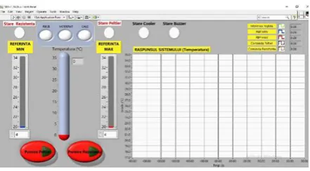
It is considered the example of the system presented with LabVIEW environment. Figure 5 shows the window displaying the front panel of the controlled process, which consists of three analogue temperature indicators, room temperature LEDs (indicating the status of all the ON / OFF elements), the system response in graphical form and manual start/stop buttons of the main actuators. These buttons have been designed to interfere with the system or to change the temperature in case of an emergency state without taking into account algorithms.

Figure 5. The front panel of the adjustment process.

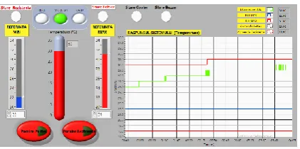
The use of the system's response in time in the form of graphically highlights the system behaviour in a more suggestive way. Viewing the real-time output response is accomplished by connecting the controller to the PC via serial communication. This allows both parameter values to be viewed and modified. On the graphic one can see the different parameters of the system, such as: the upper and lower limit of the system (set by the operator), the adjusted size, and the command of each actuator (figure 6).

Through these, the interactive user interface is provided, the controls simulate the inputs to the VI and inputs data into the block diagram, and the indicators simulate the VI outputs and display the data provided by the block diagram resulting from the execution of the program [8].

Figure 6. Secondary front panel of the adjustment process.

2) Block diagram

The window showing the block diagram corresponding to the controlled process, the front panel of which was previously displayed, is shown in figure 7.

Figure 7. Block diagram of the controlled process.

The block diagram comprises, in the workspace, the graphical representation of the functions corresponding to the objects on the front panel, and illustrates how the data stream and its processing operations circulate. Within the block diagram, the front panel objects appear as terminals, which constitute input and output ports for exchanging information with the front panel [8].

The objects in the block diagram, which highlight the operations performed by the VI program, are called nodes. Data transfer between objects in the block diagram is provided by connection links between them having different colors, styles, and thicknesses, depending on the types of data they are driving. Any connection starts from a single data source, but can be connected to one or more receivers. Also in the block diagram are so-called structures, which are graphic representations of loops and control instructions from textual programming languages.

The response of on-off controller can be observed by following the temperature evolution according to the set limits and control of the actuators.

Through the interface components placed in the front panel, it is possible to view graphic representations. The indicators are given numerical values necessary for the graphical representation, following the processing in the block diagram.

The controls are used in place of the indicators if the values required to achieve the graphical representation are received as input parameters for current VI, used as a subroutine (under VI).

The interface components, dedicated to graphic representations, are divided into two general categories:

• diagram (chart); • graph.

Charts are graphical representations of a size that changes over a period of time. Charts represent the variation of two sizes: y depending on x. In the system presented for the user interface were used 3 graphs for temperatures and humidity.

In the front panel there (first page) is only one graph showing the temperature evolution over time. In page 2, there are two other graphs, which illustrate relative humidity depending on time and current temperature depending on time.

C. Arduino platform

Arduino(figure 8) is one of the simplest to use platforms with microcontroller. We can think of it as a minicalculator (it has the power of computing a regular computer 15 years ago), being able to collect and react to environmental information.

It has 14 digital inputs / outputs and 6 analog inputs. Of the 14 digital pins on the board, 6 can also be used as PWM (Pulse-Width Modulation) outputs and the 6 analog inputs can also be used as digital pins [5].

Figure 8. Arduino UNO Development Plate [7].

D. Monitoring and controlling the system through serial connection

To achieve connectivity between the two programs, it is necessary to upload a file called LabVIEWInterface.ino on the Arduino platform, a file that must contain the DHT11 sensor code.

The LabVIEWInterface.ino file must be located in the same location as LabVIEW so that after uploading it to the microcontroller, they can be interconnected.

IV. THE PROPOSED APPLICATION FOR SIMULATING THE AUTOMATIC TEMPERATURE CONTROL SYSTEM USING THE LABVIEW AND ARDUINO PROGRAMMING

LANGUAGES

A. Physical components

In the example shown, in order to keep the room temperature as stable as possible, with small variations in the presence of various disturbances (e.g. ambient temperature) - the following elements are used: Peltier element, electrical resistance, fan pallet engine, temperature sensor, Arduino UNO development platform, relay module,

1) • Peltier element

The Peltier effect consists in the heat release or absorption at the junction between two different conductors, whereby an electric current flows through it. It has the role of cooling the enclosure by the effect outlined above, functioning as a small heat pump.

Applying a low voltage to the terminals of such a device, we can extract the heat from a junction and transfer it to the other junction based on the Peltier effect. Referring to the thermoelectric module (figure 9), one of the faces of the module is cooled while the opposite face is warming up. The heat flow through the module can be easily changed by simply reversing the sense of the supply current [7].

Figure 9. The deployed diagram of a Peltier cooling module [6].

The module (figure 10) is powered by a voltage of 12V, consuming a current of 3.8A. The maximum temperature difference between the cold and the hot part is 60 °C, the refrigeration power is 60 W and the module dimensions are: 40 x 40 x 3.8 mm. The use of this module it is justified by its main benefits: no moving parts, no noise, no maintenance and its uninterrupted operation can reach up to 30 years

2) Electrical resistance

The heating system is made of a 220V heat-resistant heat exchanger with a power of 75W, which provides heating when the room temperature is below the set limit

3) Fan Pallet Engine

In order to save electricity, an engine is used which simultaneously engages two fan pallets through a single shaft.

The one on the outside (hot side) is designed to keep the temperature as low as possible so that the temperature on the inner side (cold side) is as small as possible to achieve the quickest cooling, and more efficient. The one on the inside has the function of venting cold air inside the enclosure to speed up the cooling process.

4) Temperature Sensor

The DHT11 temperature sensor (figure 11) is a component used in the process, which senses the temperature level in the environment. This element is pre-calibrated and the output is provided as a digital signal. It connects to the programmed Arduino microcontroller. It measures the temperature between 0°C and 60°C. The DHT11 temperature and humidity sensor is suitable to our application, providing good precision, simplicity in use, and small size at a low price. It operates at a voltage between 3.3V - 5V, a maximum current of 2.5mA and does not work below 0°C.

Figure 11. DHT11 sensor [7].

5) Arduino UNO Development Platform

The development platform (figure 12) used to build the system is accessible, open-source, easy to use both in hardware and relatively small software. All devices used in the project are linked to this microcontroller:

• the digital sensor 2 is connected to the temperature sensor;

• the digital pointer 3 is connected to the buzzer;

• the cooler for outdoor cooler is connected to the digital pin 4;

• the digital pin 6 is connected to the Peltier element and a blue LED;

• the thermal resistance and red LED are connected to the digital terminal 7;

• a green LED is connected to the digital pin 8.

Figure 12. Arduino UNO Development Platform.

6) Relay module

The relay module (figure 13) is an automatic device that allows switching of an electrical circuit with a command signal.

Figure 13. Relay module [8].

7) Connection wires, power supply, radiators, breadboard, enclosure

The components that make up the automatic temperature control system were connected by means of male-father and father-to-male wires, as well as by a breadboard. The other sources are supplied at 12V with the 12V / 5A stabilizer and the relay.

The Peltier element is located between the two radiators in the enclosure. The panel is made of Plexiglas and has a length of 30cm, a width of 20cm and a height of 15cm.

B. Technical data

The closing of the contacts corresponding to the buzzer and the secondary fan is manually reset by placing the button corresponding to the actuator in the READY state (figure 14 and 15).

Starting the main actuators of the process is done manually by pressing the button corresponding to the element to be started.

Figure 15. System connection scheme.

C. System operation

In the project, the following blocks have been used: while loops, logical gates, blocks, indicators, controllers, and a number of conditions that control the other peripherals used.

If the temperature exceeds a predefined value (maximum setpoint), then the LabVIEW development environment sends the appropriate signal to Arduino and then it sends the signal to the relay module connected to pin 6 that will start the Peltier element and the fan pallet engine (connected in parallel), and at the same time the blue light turns on to show that the cooling process is carried out in the enclosure.

If the temperature drops below the set value (minimum setpoint), then the control algorithm compute the command and an appropriate signal is sent to Arduino that will connect the resistor via the relay module to increase the temperature. At the same time, the red LED will turn on to indicate that the heating process is being carried out in the enclosure.After bringing the temperature between the two previously set limits, both the actuators and the LEDs listed above will turn off and the green LED will light up, indicating a moderate temperature.

D. Experimental results. Cooling and heating on manual mode

1) Manual mode cooling:

The following experiment presented in Table I and Table II has 30 °C as start temperature. The average outside temperature of the radiator is 34.04 °C.

TABLE I. TEMPERATURE ADJUSTED BY USING SECONDARY FAN

Set temperature

(°C) Time (s) outside heatsink(°C) Temperature on the

30 00:00 34.2 29 01:22 35.4 28 02:14 35.6 27 03.06 35.2 26 03:57 34.8 TABLE II. TEMPERATURE ADJUSTED WITHOUT USING

SECONDARY FAN

Set temperature

(°C) Time (s)

Temperature on the outside heatsink(°C)

30 00:00 34.3 29 02:10 42.4 28 03:00 45.2 27 03.58 47.7

Average outdoor heat exchanger temperature (Table II) is 42.4 °C.

With an active secondary fan the average time required to lower a grade is 59 s and the average temperature on the radiator is 35.04 °C. Deactivating the secondary fan the average time required to lower a grade becomes 79 s. The average temperature on the radiator is 42.4 °C.

From experimental data, one can conclude that the average time required to lower a grade is 20 seconds lower when using the secondary fan, thus in the same period, using the fan reduced 4 degrees instead of 3 degrees.

2) Manual mode heating

Due to thermal resistance inertia, the temperature tends to increase by 4-5 °C, after disconnecting its command. In the example presented in Table III, resistance was decoupled after temperature rise by one degree (from steady state 25°C to 26°), however, it may be seen that the temperature rise by 3 degrees to the Setpoint temperature after approximately 60 seconds after uncoupling.

TABLE III. TEMPERATURECONTROLLEDBY THERMALRESISTANCE

Set temperature

(°C)

26 27 28 29

Time(s) 00:37 01:01 01:23 01:49

This thermal inertia depends on several factors, such as: the distance between the sensor and the thermal resistance, the volume of the enclosure, the operating time of the resistance, its thermal power.

A secondary fan is used and in the following two examples that are presented starting from different steady states.

a) Example 1 (Figure 16): Starting temperature: 27 °C;

Exterior radiator temperature before start: 28 °C; Ambient temperature: 27.3 °C;

Setpoint temperature: 25 °C;

Heat exchanger temperature: 35 °C;

Cooling time: 01:59 minutes.

Figure 16. Temperature set from 27 °C to 25 °C with the secondary fan turned on.

b) Example 2 (Figure 17): Starting temperature: 31 °C;

Exterior radiator temperature before start: 32.4 °C; Ambient temperature: 28.2 °C;

Setpoint temperature: 26 °C;

Heat exchanger temperature at 26 °C: 35.1 °C;

Cooling time: 03:02 minutes.

Figure 17. Temperature set from 31 °C to 26 °C with the secondary fan turned on.

The system reached a temperature of 29 °C after 1 minute and 10 seconds, the outdoor heat sink showing a value 1 degree greater than 70 seconds ago when the element was started manually. After 40 seconds the temperature dropped to 28 °C and the outside radiator has a value just 0.4 degrees more than 40 seconds ago.

The system reaches the setpoint temperature of 26 °C within 3 minutes. The total temperature reduction time of 31 °C to 26 °C is 3 minutes after the Peltier element starts up manually.

The following two experiments were done with secondary fan off:

c) Example 3 (Figure 18): Starting temperature: 28 °C;

Exterior radiator temperature at start: 29 °C; Ambient temperature: 27 °C;

Setpoint temperature: 25 °C;

Heat exchanger temperature: 43.4°C;

Cooling time: 2:48 minutes.

Figure 18. Adjustable temperature from 28 °C to 25 °C with the secondary fan off.

The system reached a temperature of 27 °C after 1 minute and 6 seconds. After 2 minutes it reached 26 °C. The system reaches the setpoint temperature of 25 °C within 2 minutes and 45 seconds and it stabilizes at

that temperature after 2 minutes and 48 seconds after the Peltier element has started manually.

The outside radiator temperature after reaching the temperature of 27 °C is 36.2 °C, at 26 °C the temperature on the radiator reaches 40.4 °C and when the room temperature stabilizes at 25 °C, value of 43.6 °C on the outside heat sink.

d) Example 4 (Figure 19): Starting temperature: 30 °C;

Exterior radiator temperature before start: 31.8 °C;

Ambient temperature: 28 °C;

Setpoint temperature: 25 °C;

External radiator temperature: 47.1 °C;

Cooling time: 04:00 minutes.

Figure 19. Temperature set from 30 °C to 25 °C with the secondary fan off.

In the above example the temperature is controlled with thermal resistance.

e) Example 5 (Figure 20): Starting temperature: 25 °C;

Ambient temperature: 28 °C;

Setpoint temperature: minimum 26 °C;

The resistance was manually disconnected after the temperature rose from 25 °C to 26 °C, but due to thermal inertia the temperature increased further in about 4 minutes by another 4 degrees.

Figure 20. Temperature set from 25 °C to 26 °C by thermal resistance.

V. CONCLUSIONS

The implementation of this application implied a careful study for the proper selection of the thermoelectric module (hot source temperature, cold source temperature, cooling power at the hot-water source, voltage and supply current).

The above system uses commercially available Peltier mode. The selection of the modules took into account the typical features, the reliability and the cost price of the modules. Thanks to this Peltier cooling technology, operating costs are reduced by up to 90% compared to compressor technology together with saving space and quietly operating due to lack of compressor and vibration.

Considering the purpose of the project mentioned in the introduction of the documentation, we can state that the target was fulfilled. Thus, the proposed theme has been physically achieved and can be used both for educational purposes to simulate the behavior of an control system and the study of its structure, as well as in more complex processes, such as controlling and measuring the temperature in a room or any another industrial application that requires temperature control without human intervention.

This project can be improved by using a PWM control signal that allows PID control algorithm in

spite of on off actuator. Moreover, the components can be replaced by some more performing ones, and the transducer with a much higher measuring precision. So, the purpose of this project has been successfully accomplished and can be easily implemented and used in practice.

REFERENCES

[1] Cîrtoaje, V., Systems Theory – Elementary analysis in time domain (in Romanian), Ed. Univ. Petrol-Gaze din Ploiești, 2015.

[2] Paraschiv, N., Rădulescu, G. Introduction in systems and computers science (in Romanian), Ed. MATRIX ROM, Bucureşti, 310 pg., 2007.

[3] Băieșu A., Automatic control technique (in Romanian), Editura MATRIX ROM, Bucuresti, 2012.

[4] Doicin B., Popescu M., Pătrăşcioiu C., PID Controller Optimal Tuning, Proceedings of the International Conference on ELECTRONICS, COMPUTERS and ARTIFICIAL INTELLIGENCE – ECAI-2016, Ploiesti, 2016, vol. 3, pp P-49 – P-52.

[5] www.robofun.ro Arduino for beginners (in Romanian). [6] Mihon L., Thermo electrical cooling systems (in Romanian),

Termotehnica, 1-2, pp 68-73, Universitatea Politehnica, Timisoara 2004.

[7] www.optimusdigital.ro