STABILITY AND BOUNDEDNESS ANALYSIS OF A SYSTEM OF RLC CIRCUIT WITH RESPONSE

ISSN: 1311-1728 (printed version); ISSN: 1314-8060 (on-line version) doi:_{http://dx.doi.org/10.12732/ijam.v33i1.4}

STABILITY AND BOUNDEDNESS ANALYSIS OF A SYSTEM OF RLC CIRCUIT WITH RESPONSE

A.L. Olutimo1§, I.D. Omoko2 1,2_{Department of Mathematics}

Lagos State University Ojo - 23401, NIGERIA

Abstract: This paper presents a stability and boundedness analysis of a sys-tem of RLC circuit modeled using a time varying state-space method. Stability problem analysis is very important in RLC circuits. There is some potential for a response characterizing the system of RLC circuit to approach infinity when subjected to certain types of inputs. Unstable circuit causes damage to electrical systems. Analysis of problems of such system stability is carried out using the Lyapunov’s theory. In this paper, we provide in simple form, con-ditions which ensure the stability and boundedness of the state variables xi(t) (i= 1,2) characterizing the system of RLC circuit using Lyapunov’s second or direct method.

AMS Subject Classification: 34D40, 34D20, 34D20, 34C25

Key Words: RLC circuits; state variables; stability and boundedness of system circuit; Lyapunov function

1. Introduction

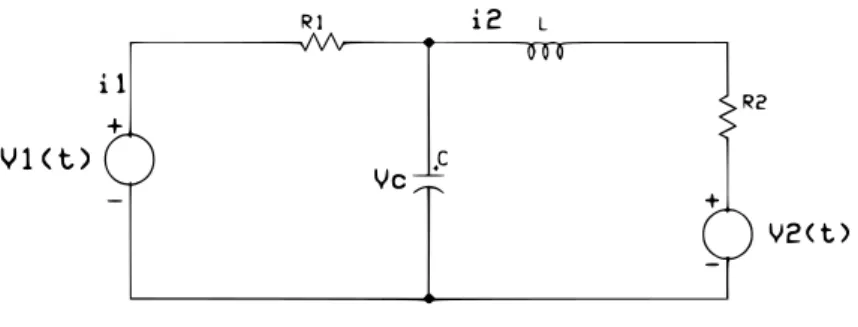
An RLC circuit is a resonant or a tuned circuit consisting of a resistor (R), an inductor (L) and a capacitor (C) connected in series or parallel. An RLC circuit can be described by a linear second order differential equation for circuit analysis. The importance of this is that its characterization is given by its transfer function, which is the frequency domain equivalent of the time domain input-output relation. The knowledge of the interior parameters of the circuit

Received: July 22, 2019 c 2020 Academic Publications

Figure 1: RLC Circuit

is not considered but rather to the control of the closed-loop behavior when feedback control is used. RLC circuit systems are widely applied in electro-mechanical systems and other technical field of application. The qualitative theory of such system is more complicated to analyze. If we determine input, the state variables and their response vary depending on the circuit. The out response tends to zero as time tends to infinity. If out response of such a system circuit approaches infinity, the circuit is said to be unstable. This undesirable case can be detected theoretically and eliminated at development stage. To address this problem, we make use of Lyapunov theory. Results obtained may be useful to researchers who may want to use it for the development of more general cases like coupled circuits.

The energy storage elements of a system are what make the system dynamic. The flow of energy into and out of a storage element occurs at a finite rate is described by a differential equation relating the derivative of the energy storage variable (a state variable) to other power variable of the element. There are two independent energy storages in RLC circuit, the capacitor which stores energy in an electric field and the inductor which stores energy in a magnetic field. The state variables are the energy storage variables of these two elements, Vc and

ViL. According to Peng and Pileggi [8], state variables are the minimum set of variables that fully describe the system circuit and its response to any given set of inputs. By this, it shows that the qualitative properties of state-determined system like Fig.1 is completely characterized by the stability and boundedness of the set of xi(t) (i= 1,2) variables.

x₂(t) =Vc(t). It is also necessary to apply Kirchhoff’s laws and by KCL and KVL in Morris [4], we obtain the following system of differential equations:

˙

x1(t) = −

R2

L x1(t) +

1

Lx2(t)− V2(t)

L ,

˙

x₂(t) = −1

Cx1(t)−

1

CR1

x₂(t) +V1(t)

CR1

. (1)

Equation (1) is linear heterogeneous system of two differential equations of the first order which can be represented in matrix notation as

d dt

x1(t)

x2(t)

=

−R2

L L1

−_C1 −_CR1 1

x1(t)

x2(t)

+

0 −_L1

1 CR1 0

V1(t)

V₂(t)

. (2)

Now, we represent (2) as a linear vector differential equation of order one,

˙

X=AX+F(t), (3)

with load. And very recently, Piriadarshani and Sujitha [7] investigated the stability of feedback control system using transfer function while Lenka [2] es-tablished new stability conditions for certain class of nonautonomous fractional order systems using time varying Lyapunov functions. Thus, our problem in Fig. 1 is best treated since it has been reduced to stability problem according to Lyapunov’s equations in (1). This Lyapunov’s second method lies in con-structing a scalar function, Φ such that it is positive definite and its derivative ˙Φ, along the system (1) is negative-semi definite. When these properties of Φ and ˙Φ are shown to be satisfied according to Lyapunov’s theory (Demidovich [1], Yoshizawa [12]), then the behavior of the system circuit is known. The construction of a Lyapunov function Φ, which is a quadratic form satisfying the requirements for Φ and ˙Φ for discussing the stability and boundedness of thexi(t) variables of the linear vector differential equation (3) forF(t) = 0 and

F(t)6= 0 respectively is obtained. It must be noted here that the physical mean-ing of Lyapunov function is not considered. In known cases Lyapunov functions were obtained as abstract mathematical approach results, see Pai [6]. Also, in this study we assume that physical meaning availability is not connected with function efficiency.

2. Stability analysis Assumptions:

In addition to the basic assumption imposed on the elements R, L and C

in (1), we also assume that

(i) R22

L + R1R2

L + R2

CR1 +

1

C >0 and (ii) |V₁(t)−V₂(t)| ≤ρ(t),

where V₁(t) and V₂(t) are the input and reverse voltages respectively in the circuit.

To establish our result, we employ the following scalar function Φ = Φ(x1, x2) defined by

2Φ(x1, x2) = R2+

L

CR₁ +R1

x2₁+ 2x1x2+

CR1

L x

2

2. (4)

From (4), it is clear that Φ(0,0) = 0. Φ in (4) can be arranged as follows,

2Φ(x1, x2) = R2+R1x21+

L CR1

x1+

CR1

L x2 2

It is obvious from (5) that the function Φ defined in (4) is a positive definite function. Hence, there is a positive constant D1 such that

Φ(x1, x2)≥D1(x21+x22). (6)

Now, consider the case of a natural process where dissipation is absent that is,

F(t) = 0 in (3).

On using (4), a direct differentiation of dΦ_dt along the system (1) gives after simplification of Φ, yields

˙Φ(t)≤ − R

2 2

L + R1R2

L +

R2

CR1 + 1

C

x2₁. (7)

It follows that dΦ(x1,x2)

dt = 0 if and only if x1 = 0,

dΦ(x1,x2)

dt <0 for x1 6= 0 and Φ(0,0) ≥0.

Thus, the system of RLC circuit in Fig. 1 is stable according to Lyapunov’s theory if Assumption (i) is satisfied from the timeto to t→ ∞,t≥to. In this case, the impulse response approaches zero ast→ ∞.

3. Boundedness analysis

We now consider the case F(t) 6= 0 in (3) where dissipation is present due to external conductive connections or elements.

The conclusion of (7) can be revised as follows

˙Φ(t) = dΦ

dt ≤k1|V1−V2|x1+k2|V1−V2|x2,

wherek1= max_CRV1₁,R_L2 +_CR1₁ + R_L1 and k2 =_L1 . By noting Assumption (ii), we have

˙Φ(t)≤ k1|x1|+k2|x2|

ρ(t).

On using inequality |x| ≤1 +x2, we get

˙Φ(t)≤k3 2 +x21+x22

ρ(t),

wherek3= max{k1, k2}. Thus,

˙

Since D₁(x2₁+x2₂)≤Φ(x₁, x₂), by (6) it follows that

˙Φ(t)≤2k3ρ(t) +k3D1−1Φ(x1, x2)ρ(t). (8) We assume that the input is conditioned to be finite and controllable, thus we have that

Z t

0

ρ(s)ds

≤D2, D2 >0 for allt≥0.

Integrating (8) from 0 to t with the above assumption and Gronwall-Reid-Bellman inequality, we obtain

Φ(x1, x2)≤ Φ(0,0) + 2k3D2exp k3D₁−1D2. (9)

Now, since the right hand side of (9) is a constant and Φ(x1, x2) → ∞ as

x2₁+x2₂→ ∞, it follows that there exist a positive constantD3 such that

|x1(t)| ≤D3 and |x2(t)| ≤D3 for t≥0.

Thus, this implies that every bounded input produces a bounded output if the stated assumptions are satisfied.

Stability analysis for system (1)

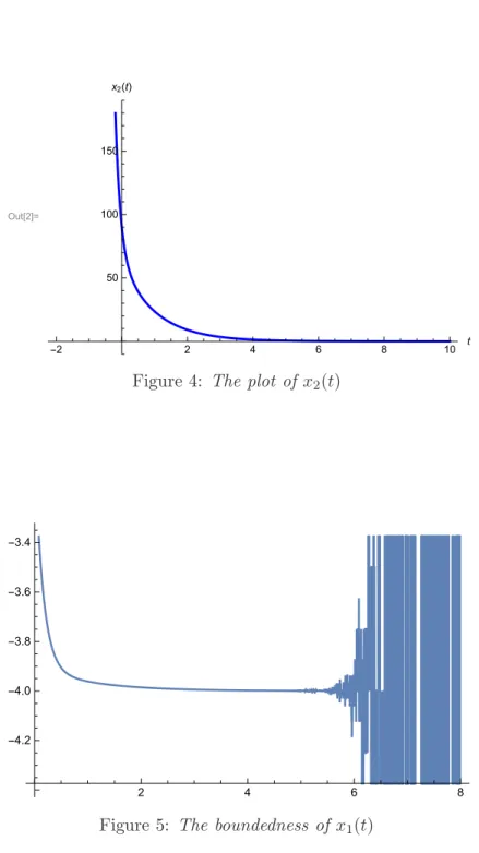
The plot of x1(t), x2(t) of equations (1) which are the critical variables characterizing the RLC circuit in Fig. 1. is shown in Fig. 2, Fig. 3 and Fig. 4 below. It is very clear from Fig. 2, Fig. 3 and Fig. 4 that Assumption (i) obtained by the Lyapunov functional (4) is satisfied for all values of R1, R2, C and Lalong the graphs and x1(t),x2(t) are asymptotically stable ast→ ∞.

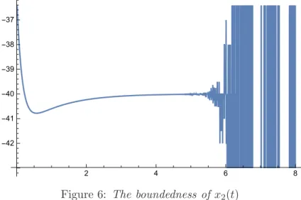
In Fig. 5 and Fig. 6, as Assumption (i) and (ii) are satisfied, x1(t), x2(t) are bounded as t→ ∞. The boundedness ofx1(t), x2(t) obviously depend on

R1, R2, C and L. Our result shows that x1(t), x2(t) are bounded by a single constant if the Assumption (i) and (ii) are satisfied but the physical effect on the external conductive elements or connections is not considered.

Conclusion

Out[4]=

2 4 6 8

-0.06 -0.04 -0.02 0.02 0.04 0.06

x₂[t]

x₁[t]

Figure 2: The plot of x₁(t) in (blue) and x₂(t) in (red) on the same axes

Out[1]=

2 4 6 8 t

-2.0

-1.5 -1.0 -0.5 0.5 1.0

x1(t)

Out[2]=

-2 2 4 6 8 10 t

50 100 150 x

✷(

t)

Figure 4: The plot of x₂(t)

2 4 6 8

-4.2

-4.0

-3.8

-3.6

-3.4

2 4 6 8

-42

-41

-40

-39

-38

-37

Figure 6: The boundedness of x2(t)

References

[1] B.P. Demidovich, Lectures about Mathematical Stability Theory, Nauka, Moscow (1967).

[2] B.K. Lenka, Time-varying Lyapunov functions and Lyapunov stability of nonautonomous fractional order systems,International Journal of Appled Mathematics,32, No 1 (2019), 111-130; DOI: 10.12732/ijam.v32i1.11. [3] A.M. Liapunov, Stability of Motion, Academic Press, London (1966).

[4] N.M. Morris, F.W. Senior, Electric Circuits, Macmillan, Hong Kong (1991).

[5] A.L. Olutimo, Stability analysis of a system of DC servo motor with load, Engineering Math. Letters,6 (2017), 1-7.

[6] M.A. Pai, Power System stability studies by Lyapunov-Pupov Approach, In: 5th IFAC World Congress, Paris (1972).

[7] D. Piriadarshani, S.S. Sujitha, The role of transfer function in the study of stability analysis of feedback control system with delay, Interna-tional Journal of Appled Mathematics, 31, No 6 (2018), 727-736; DOI: 10.12732/ijam.v31i6.3.

[9] Y. Qin, Y. Liu, L. Wang, Stability of Motion for Dynamic Systems with Delay, Academic Press, Beijing (1966).

[10] C. Tunc, Some remarks on the stability and boundedness of solutions of certain differential equations of fourth-order,Comp. Appl. Math.,26, No 1 (2007), 1-17.

[11] H. Yao, W. Meng, On the stability of solutions of certain nonlinear third order delay differential equations,Int. J. Nonlinear Science,6, No 3 (2008), 230-237.