ISSN: 1311-1728 (printed version); ISSN: 1314-8060 (on-line version) doi:http://dx.doi.org/10.12732/ijam.v30i5.2
SINGLE MACHINE SLACK DUE-WINDOW SCHEDULING WITH LINEAR RESOURCE ALLOCATION, AGING EFFECT,
AND A DETERIORATING RATE-MODIFYING ACTIVITY
Bo Cheng1§, Ling Cheng2
1Department of Applied Mathematics
School of Finance
Guangdong University of Foreign Studies Guangzhou, 510420, P.R. CHINA
2School of Electrical and Information Engineering
University of the Witwatersrand Private Bag 3, Wits. 2050 Johannesburg, SOUTH AFRICA
Abstract: In this paper, we consider the slack due-window method and inves-tigate single machine scheduling with a deteriorating rate-modifying activity, linear resource allocation and aging effect. The objective is to minimize the to-tal cost caused by the due-window location, the due-window size, the earliness and tardiness with respect to a slack due-window, and resource consumption. We provide a polynomial-time algorithm to solve the corresponding problem.
AMS Subject Classification: 90B35
Key Words: aging effect, due-window, rate-modifying activity, resource al-location, scheduling
1. Introduction
In the studies on operations management, a good customer service usually requires jobs completed as close as possible to their due-dates. A time interval is assigned in the supply contract so that a job finished within this period will
Received: August 8, 2017 c 2017 Academic Publications
be considered on time and not be penalized. This period is called the due-window of a job (cf. [1, 2]). The due-due-window assignment methods include common due-window, slack due-window (also called common flow allowance) and others.
Scheduling theory for jobs with changeable job processing times has been developed steadily in the last decade. The single machine common due-window assignment problem with deteriorating jobs and learning effect was studied by [3] and polynomial-time algorithms were given to minimize the total costs for earliness, tardiness, window location and window size. The parallel problem for the slack due-window model was investigated by [4]. Other scheduling problems with the aging effect were studied by [5, 6, 7].
The effect of allocating additional resources on job processing times was also extensively investigated by [8, 9, 10] and others. A linear function taking the amount of allocated resource as the input parameter was proposed to quantify the effect of additional resources on job processing times. For example, in a linear resource consumption model, the actual processing time of a job is determined by
˜
p=p−cu, 0≤u≤u <¯ p
c, (1)
where ˜pis the actual processing time,pis the non-compressed (normal) process-ing time,cis the positive compression factor, uis the actual resource allocated to the job, and ¯u is the maximum resource that could be allocated to the job. For the linear resource consumption model in this paper, we remove the upper bound on ¯uin (1), since the new one without the upper bound is more general. Machine scheduling with a rate-modifying activity (RMA) was initially in-vestigated by [11]. In this paper, at most one RMA can be scheduled before or after any job except that it is unnecessary to schedule a RMA after the last job. The scheduler decides when to perform the RMA. However, the RMA cannot interrupt any job. It means the RMA can be scheduled either before or after a job.
The combinations of the above-mentioned settings have been further in-vestigated. [12] studied common due-window assignment and scheduling with time-dependent deteriorating jobs and a maintenance activity, and [9, 10] in-vestigated the scheduling problem with resource allocation, aging effect and a deteriorating RMA based on common due-window method. [13] considered the slack due-window assignment and scheduling taking into account variable processing-time jobs and a rate-modifying activity.
position-dependent deteriorating jobs with a RMA. To our best knowledge, this problem has not been studied in literatures.
The rest of this paper is organized as follows. A description of the problem under study is given in Section 2. In Section 3 a few important lemmas and properties are presented. In the same section, a polynomial-time solution is given. A numerical example is presented to demonstrate the polynomial-time solution in Section 4. The research is concluded and future study is foreseen in the last section.
2. Model Formulation
In the models considered in this paper,nindependent and non-preemptive jobs J1, J2, . . . , Jn and at most one RMA are scheduled on a single machine. All
the jobs and the RMA can be scheduled at time zero. Let pj be the normal
processing time of job Jj. The predetermined parameters of job Jj are the
job-dependent aging factoraj and the maximum available resource amount ¯uj.
Let pjr denote the actual processing time of Jj scheduled in the rth position.
The actual resource allocated to jobJj is denoted asuj. For the linear resource
consumption model, the actual processing time of jobJj is determined by
pjr =pjraj−cjuj, (2)
wherecj is the positive compression rate of job Jj, 0≤uj ≤u¯j and pjr≥0.
The RMA duration is determined by f(t) = b+σt, where b > 0 is the basic RMA time, σ ≥ 0 is the RMA deterioration rate, and t is the starting time of the RMA. The modifying rate of job Jj is notated by λj. After the
RMA, the machine will revert to its initial conditions, machine deterioration will start anew, and the processing time of jobJj will be multiplied byλj. In
the proposed model, we assume the RMA can improve the efficiency of a job (thereforeλj takes a value in (0, 1]).
The due-window of jobJj is specified by a pair of non-negative real numbers
[dj, d′j] such that dj ≤d′j, wheredj and d′j are the beginning and ending times
of the due-window respectively. For the slack due-window method, dj and d′j
are determined by
dj =pjr+q, (3)
and
d′j =pjr+q′, (4)
Then the due-window sizeDj =dj−d′j =q′−q, forj= 1, . . . , n, is identical
for all the jobs. Let D=Dj.
For a given schedule π, Cj denotes the completion time of job Jj, Ej =
max{0, dj −Cj} is the earliness value of job Jj, and Tj = max{0, Cj −d′j} is
the tardiness value of jobJj. To this end, we can create the following total cost
function
Z =
n
X
j=1
(αEj +βTj+γdj +δD) +θ n
X
j=1
Gjuj, (5)
which takes into account (i) earliness Ej, (ii) tardiness Tj, (iii) the starting
time of the due-window dj, (iv) the due-window size D, and (v) the resource
allocation. We further define α >0, β > 0, γ > 0 and δ >0 representing the earliness, tardiness, due-window starting time and due-window size costs per unit time respectively. For the resource consumption cost,Gj is defined as the
per unit resource cost for job Jj and θ is a constant weight which is specified
by the decision-maker.
The general objective is to determine the optimal job sequence, the optimal location of the RMA, the optimal resource consumption and the optimalq and q′ to minimize the total cost function
Z =Z(π, u, q, q′) =
n
X
j=1
(αEj+βTj+γdj +δD) +θ n
X
j=1
Gjuj. (6)
The problems under study are denoted as
1|SLK, pjr=pjraj−cjuj,
RM A| n
X
j=1
(αEj +βTj+γdj +δD) +θ n
X
j=1
Gjuj,
whereSLKandRM Adenote the slack due-window method and rate-modifying activity, respectively.
3. Optimal Solution
In this section some properties for an optimal schedule are obtained.
Lemma 1. IfC[r]≥d′
[r] holds, thenC[r+1]≥d′[r+1].
Lemma 2. IfC[r]≤d[r] holds, thenC[r−1]≤d[r−1].
Consider a job sequenceπand a resource consumption wayu= (u1, u2, . . . ,
un). Assume that C[s]≤q ≤C[s+1] andC[t]≤q′ ≤C[t+1]. Then the total cost
Z is a linear function of q and q′, and thus an optimum is obtained either at q=C[s]or q=C[s+1]and either at q′=C
[t] or q′ =C[t+1].
Lemma 3. (i) For any given job sequenceπ and resource consumptionu, there exists an optimal schedule in which the values of q and q′ coincide with the completion times of thek-th and l-th jobs (l≥k) in the sequence.
(ii) An optimal schedule starts at time zero and contains no idle time be-tween consecutive jobs.
For a numbera,thesymbol⌊a⌋denotes the largest integer not more thana.
Lemma 4. k=jn(δ−γ)α k and l=jn(β−δ)β k.
By Lemma 4, the values ofkand lcan be calculated. Let ibe the position of the last job preceding the RMA. If the position of the RMA is beforek(i.e., i < k), then the total cost is given by
Z =
n
X
r=1
(αE[r]+βT[r]+γd[r]+δD) +θ n
X
j=1
Gjuj
=α
k
X
r=1
(pjr+q−C[r]) +β n
X
r=l+1
(C[r]−pjr−q′)
+γ
n
X
r=1
(q+pjr) +nδ(q′−q) +θ n
X
j=1
Gjuj
=α
k
X
r=1
jpjr+αi(b+σ i
X
r=1
pjr) +β n
X
r=l+1
(n−r)pjr
+γ(n(b+σ
i
X
r=1
pjr) + (n+ 1) k
X
r=1
pjr+ n
X
r=k+1
+nδ
l
X
r=k+1
pjr+θ n
X
j=1
Gjuj
=nbγ+αib+
n
X
r=1
wrpjr+θ n
X
j=1
Gjuj, (7)
where
wr=
αr+αiσ+γnσ+ (n+ 1)γ, if r = 1,2, ..., i,
αr+ (n+ 1)γ, if r =i+ 1, i+ 2, ..., k,
γ+nδ, if r =k+ 1, k+ 2, ..., l,
β(n−r) +γ, if r =l+ 1, l+ 2, ..., n.
(8)
Ifk≤i < l, then we have
Z =α
k
X
r=1
rpjr+β n
X
r=l+1
(n−r)pjr+γ (n+ 1) k
X
r=1
pjr+ n
X
r=k+1
pjr
!
+nδ(b+σ
i
X
r=1
pjr) +nδ l
X
r=k+1
pjr+θ n
X
j=1
Gjuj
=nδb+
n
X
r=1
wrpjr+θ n
X
j=1
Gjuj,
(9)
where
wr =
αr+γ(n+ 1) +nδσ, 1≤r≤k, γ+nδσ+nδ, k < r≤i,
γ+nδ, i < r≤l,
β(n−r) +γ, l < r≤n.
(10)
Ifl≤i≤n, then we have
Z =α
k
X
r=1
rpjr+β n
X
r=l+1
(n−r)pjr+ (n−i)(b+σ i
X
r=1
pjr)
!
+γ (n+ 1)
k
X
r=1
pjr+ n X r=k+1 pjr ! +nδ l X r=k+1
pjr+θ n
X
j=1
Gjuj
= (n−i)βb+
n
X
r=1
wrpjr+θ n
X
j=1
Gjuj,
where
wr =
αr+β(n−i)σ+γ(n+ 1), 1≤r ≤k, β(n−i)σ+γ+nδ, k < r ≤l, β(n−r) +β(n−i)σ+γ, l < r ≤i,
β(n−r) +γ, i < r≤n.
(12)
Note that when i = n there is no RMA scheduled since by then all jobs are finished.
For the linear resource consumption models, we have
pjr=
(
pjraj−cjuj, r ≤i,
λjpj(r−i)aj−cjuj, r > i,
(13)
and thus
Z =M +
n
X
r=1
wrpjηjr+ n
X
r=1
(θGj−wrcj)uj, (14)
where M =
nbγ+αib, i < k, nδb, k≤i < l, (n−i)βb, l≤i≤n,
(15)
and
ηjr=
(
raj, r≤i,
λj(r−i)aj, r > i.
(16)
Therefore, minimizing the objective functionZ is equivalent to minimizing Z′:
Z′ =
n
X
r=1
wrpjηjr+ n
X
r=1
(θGj−wrcj)uj. (17)
Since pjr>0, we have
pjraj−cjuj ≥0 if r ≤i (18)
and
λjpj(r−i)aj−cjuj ≥0 if r > i. (19)
Set
u′j =
min{uj,pjr aj
cj }, if r≤i,
min{uj,λjpj(r−i) aj
cj }, if r > i.
Therefore, we have uj ≤u′j.
We see the optimal resource consumption for a job depends on the sign of θGj−wrcj. Letu∗j be the optimal resource consumption for jobJj. Then,
u∗j =
u′j, if θGj−wrcj <0,
uj ∈[0, u′j], if θGj−wrcj = 0,
0, if θGj−wrcj >0.
(21)
To this end we can define the elementχjrin an assignment matrix as follows:
χjr =
(
wrpjηjr, if θGj−wrcj ≥0,
wrpjηjr+ (θGj −wrcj)u′j, if θGj−wrcj <0,
(22)
and
zjr=
(
1 if job Jj is scheduled in therth position
0 otherwise. (23)
To minimize the problem 1|SLK, pjr=pjraj−cjuj, RM A|Pnj=1(αEj+βTj+
γdj+δD) +θPnj=1Gjuj is equivalent to minimizing the following Assignment
Problem, which can be solved in time complexity O(n3):
min
n
X
j=1 n
X
r=1
χjrzjr
s.t.
Pn
j=1zjr = 1, r = 1,2, . . . , n,
Pn
r=1zjr= 1, j = 1,2, . . . , n,
zjr= 0 or 1, j, r = 1,2, . . . , n.
(24)
Here (24) presents a 0-1 integer linear programming problem, which guar-antees that each position has one job scheduled and each job is scheduled once. The following solution algorithm has anO(n4) time complexity.
Algorithm 1. Solution algorithm for the problem 1|SLK, pjr =pjraj−
cjuj, RM A|Pnj=1(αEj+βTj +γdj+δD) +θPnj=1Gjuj.
1 SET k=j n(δ−γ)α k, l=j n(β−δ)β k.
2 FOR each position i= 0,1, . . . , n available to allocate rate-modifying activity
4 DETERMINE the positional weight wr
5 END FOR
6 FOR each job j= 1,2, . . . , n
7 FOR each position r = 1,2, . . . , n in a schedule
8 DETERMINE the value χjr according to (22)
9 END FOR
10 END FOR
11 DETERMINE a local optimal schedule of the
assignment problem described in (24) and its
total cost 12 END FOR
13 DETERMINE the global optimal schedule with the minimum total cost
Theorem 1. Algorithm 1 solves the problem1|SLK, pjr=pjraj−cjuj,
RM A|Pn
j=1(αEj+βTj +γdj+δD) +θPnj=1Gjuj inO(n4) time.
Proof. The correction of Algorithm 1 is guaranteed by Lemmas 4 and the derivation from (7) to (24). The time complexity from Step 3 to Step 11 is O(n3). In the outer loop from Step 2 to Step 12, position index i takes on integer values between 0 to n. Hence, the time complexity for solving the 1|SLK, pjr =pjraj−cjuj, RM A|Pnj=1(αEj+βTj+γdj+δD)+θPnj=1Gjuj
problem isO(n4).
In most studies of the linear resource model, an upper bound on ¯u is stated as (1). In this paper we remove this constraint and consider a more general case, to which Algorithm 1 gives a solution.
4. Numerical Example
In this section, Algorithm 1 for the linear resource model is demonstrated by the following example.
Example 1. There aren= 7 jobs. The initial setup of all jobs is illustrated by Table 1.
j 1 2 3 4 5 6 7
pj 45 18 48 46 50 43 21
aj 0.3 0.5 0.25 0.3 0.15 0.4 0.2
cj 3 2 3 4 3 4 2
λj 0.58 0.84 0.45 0.55 0.38 0.64 0.75
Gj 34 40 25 38 24 48 42
uj 99 7 7 6 6 6 7
Table 1: The settings in Example 1.
Solution: By Lemma 4, we have the locations of k = jn(δ−γ)α k = 3 and
l=jn(β−δ)β k= 5.
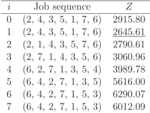
As shown in Table 2, all the local optimal job sequences and the correspond-ing total costs are presented, among which the optimal total cost is underlined. The global optimal solution for this example includes the following: (i) the job sequence is (2, 4, 3, 5, 1, 7, 6) and the corresponding job starting time and ac-tual processing time are (0, 19.40, 20.70, 25.39, 29.79, 29.79, 37.52) and (4.00, 1.30, 4.69, 4.40, 0, 7.73, 56.35), respectively; (ii) the slack window parameters are q = 25.39 and q′ = 29.79; (iii) the RMA is located immediately after the first job (i.e. Job J2), starting at time t= 4.00 and ending at time t = 19.40
(maintenance duration 15.40); (iv) the optimal resource consumption of each job is (13.19, 7.00, 7.00, 6.00, 6.00, 0, 7.00); (v) the total cost isZ = 2645.61.
i Job sequence Z
0 (2, 4, 3, 5, 1, 7, 6) 2915.80 1 (2, 4, 3, 5, 1, 7, 6) 2645.61 2 (2, 1, 4, 3, 5, 7, 6) 2790.61 3 (2, 7, 1, 4, 3, 5, 6) 3060.96 4 (6, 2, 7, 1, 3, 5, 4) 3989.78 5 (6, 4, 2, 7, 1, 3, 5) 5616.00 6 (6, 4, 2, 7, 1, 5, 3) 6290.07 7 (6, 4, 2, 7, 1, 5, 3) 6012.09
5. Conclusion
We have investigated a single machine scheduling and slack due-window assign-ment problem with linear resource allocation, aging effect and a deteriorating rate-modifying maintenance activity. The objective is to minimize the total cost caused by the due-window location, due-window size, earliness, tardiness and resource consumption.
Further research may consider the problem with other performance mea-sures, or the problem with multiple rate-modifying maintenance activities.
References
[1] T. C. E. Cheng, Optimal common due-date with limited completion time deviation, Computers &Operations Research,15(1988), 91–96.
[2] S. Liman, S. Panwalkar, and S. Thongmee, Common due window size and location determination in a single machine scheduling problem,Journal of the Operational Research Society, 49(1998), 1007–1010.
[3] J.-B. Wang and C. Wang, Single-machine due-window assignment problem with learning effect and deteriorating jobs, Applied Mathematical Mod-elling,35(2011), 4017–4022.
[4] J.-B. Wang, L. Liu, and C. Wang, Single machine SLK/DIF due window assignment problem with learning effect and deteriorating jobs, Applied Mathematical Modelling,37 (2013), 8394–8400.
[5] S.-J. Yang, D.-L. Yang, and T. C. E. Cheng, Single-machine due-window assignment and scheduling with job-dependent aging effects and deterio-rating maintenance, Computers &Operations Research, 37 (2010), 1510– 1514.
[6] C.-L. Zhao and H.-Y. Tang, Single machine scheduling with general job-dependent aging effect and maintenance activities to minimize makespan,
Applied Mathematical Modelling,34 (2010), 837–841.
[7] R. Rudek, Scheduling problems with position dependent job processing times: computational complexity results, Annals of Operations Research,
196(2012), 491–516.
[9] M. Ji, J. Ge, K. Chen, and T. Cheng, Single-machine due-window assign-ment and scheduling with resource allocation, aging effect, and a deteri-orating rate-modifying activity, Computers & Industrial Engineering, 66
(2013), 952–961.
[10] B. Cheng and L. Cheng, Note on single-machine due-window assignment and scheduling with resource allocation, aging effect, and a deteriorating rate-modifying activity, Computers & Industrial Engineering, 78 (2014), 320–322.
[11] C.-Y. Lee and V. Leon, Machine scheduling with a rate-modifying activity,
European Journal of Operational Research, 128(2001), 119–128.
[12] T. C. E. Cheng, S.-J. Yang, and D.-L. Yang, Common due-window as-signment and scheduling of linear time-dependent deteriorating jobs and a deteriorating maintenance activity, International Journal of Production Economics,135 (2012), 154–161.
[13] B. Mor and G. Mosheiov, Scheduling a maintenance activity and due-window assignment based on common flow allowance,International Jour-nal of Production Economics,135 (2012), 222–230.
[14] G. Mosheiov and D. Oron, Job-dependent due-window assignment based on a common flow allowance,Foundations of Computing and Decision Sci-ences,35(2010), 185–195.