How To Write A New Vertical Diffusion Package

A New Vertical Diffusion Package with an Explicit Treatment of

Entrainment Processes

SONG-YOUHONG ANDYIGN NOH

Department of Atmospheric Sciences, Global Environment Laboratory, Yonsei University, Seoul, South Korea

JIMYDUDHIA

Mesoscale and Microscale Meteorology Division, National Center for Atmospheric Research, Boulder, Colorado

(Manuscript received 11 April 2005, in final form 13 December 2005) ABSTRACT

This paper proposes a revised vertical diffusion package with a nonlocal turbulent mixing coefficient in the planetary boundary layer (PBL). Based on the study of Noh et al. and accumulated results of the behavior of the Hong and Pan algorithm, a revised vertical diffusion algorithm that is suitable for weather forecasting and climate prediction models is developed. The major ingredient of the revision is the inclusion of an explicit treatment of entrainment processes at the top of the PBL. The new diffusion package is called the Yonsei University PBL (YSU PBL). In a one-dimensional offline test framework, the revised scheme is found to improve several features compared with the Hong and Pan implementation. The YSU PBL increases boundary layer mixing in the thermally induced free convection regime and decreases it in the mechanically induced forced convection regime, which alleviates the well-known problems in the Medium-Range Forecast (MRF) PBL. Excessive mixing in the mixed layer in the presence of strong winds is resolved. Overly rapid growth of the PBL in the case of the Hong and Pan is also rectified. The scheme has been successfully implemented in the Weather Research and Forecast model producing a more realistic structure of the PBL and its development. In a case study of a frontal tornado outbreak, it is found that some systematic biases of the large-scale features such as an afternoon cold bias at 850 hPa in the MRF PBL are resolved. Consequently, the new scheme does a better job in reproducing the convective inhibition. Because the convective inhibition is accurately predicted, widespread light precipitation ahead of a front, in the case of the MRF PBL, is reduced. In the frontal region, the YSU PBL scheme improves some characteristics, such as a double line of intense convection. This is because the boundary layer from the YSU PBL scheme remains less diluted by entrainment leaving more fuel for severe convection when the front triggers it.

1. Introduction

The approach pioneered by Troen and Mahrt (1986, hereafter TM86), the so-called “nonlocalK” approach, considers the countergradient fluxes in a model that diagnoses the PBL depth and then constrains the ver-tical diffusion coefficientKto a fixed profile over the depth of the PBL. This scheme is supported by the large-eddy simulation results (Wyngaard and Brost 1984), and has been successfully applied to general cir-culation models as well as numerical weather prediction

models with further generalization and reformulation (Holtslag and Boville 1993; Hong and Pan 1996, here-after HP96). It is also applied to the upper-ocean boundary layer (Large et al. 1994).

The nonlocal boundary layer vertical diffusion scheme implemented by HP96 for the operational Me-dium-Range Forecast (MRF) model revealed a consis-tent improvement in the skill of precipitation forecasts over the continental United States (Caplan et al. 1997). Features of monsoonal precipitation and associated large-scale features over India were greatly improved compared with the results from a local approach (Basu et al. 2002). In the fifth-generation Pennsylvania State University–National Center for Atmospheric Research (PSU–NCAR) Mesoscale Model (MM5; Grell et al. 1994), this scheme, the MRF PBL, has been widely

Corresponding author address:Song-You Hong, Department of Atmospheric Sciences, Yonsei University, Seoul 120-749, South Korea.

E-mail: [email protected]

2318 M O N T H L Y W E A T H E R R E V I E W VOLUME134

© 2006 American Meteorological Society

selected because it provides a realistic development of a well-mixed layer despite its simplicity. For example, Farfán and Zehnder (2001) selected this scheme based on its capability in simulating the structure and diurnal variability of the boundary layer over land and ocean. Bright and Mullen (2002) compared four boundary layer schemes and concluded that the MRF PBL scheme, together with the Blackadar scheme, correctly predicted the development of the deep, monsoon PBL, and consequently did a better job of predicting the con-vectively available potential energy (CAPE). The re-sults of two years of real-time numerical weather pre-diction over the Pacific Northwest also showed that the scheme could be applicable for a wide range of hori-zontal grid spacings without a significant defect (Mass et al. 2002). Because of the reasons above, the MRF PBL scheme was selected as a standard option for the vertical diffusion process in the Weather Research and Forecast (WRF) model.

While the MRF PBL scheme has been extensively evaluated in the National Centers for Environmental Prediction (NCEP) operational models and MM5, some deficiencies have been reported. A typical prob-lem is that the scheme produces too much mixing when wind is strong. Persson et al. (2001) showed that in comparison with aircraft data over the oceans, the simulation of a maritime storm using the MRF PBL scheme shows a significant defect by producing too deep a boundary layer. Mass et al. (2002) determined that the scheme produced too much mixing and results in excessive winds near the surface at night. Braun and Tao (2000) showed that in the simulation of Hurricane Bob (in 1991) the MRF PBL scheme produced the weakest storm compared with other PBL schemes available in MM5, which was because the lower PBL is dried as a result of excessively deep vertical mixing. Bright and Mullen (2002) demonstrated that the MRF PBL scheme weakens the convective inhibition, which in turn provides a limiting factor in the model’s ability to produce accurate quantitative precipitation forecasts during the southwestern monsoon over the United States.

Recently, Noh et al. (2003, hereafter N03) proposed some modifications to the TM86 method based on large-eddy simulation (LES) data. Major modifications made by N03 include the following: 1) an explicit treat-ment of the entraintreat-ment process of heat and momen-tum fluxes at the inversion layer, 2) using vertically varying parameters in the PBL such as the Prandtl number and mixed-layer velocity scale, and 3) the in-clusion of nonlocal-K mixing for momentum. N03 re-vealed that the first factor is the most critical to the improvement, which resolves the problems of too much

mixing with strong wind shear and too little mixing in the convection-dominated PBL.

This paper documents a revised vertical diffusion package after HP96, focusing on the inclusion of con-cepts introduced by N03 for mixed layer turbulence. An overview of the performance of the MRF PBL is given in section 2. Changes of free atmospheric diffu-sion processes after HP96 as well as mixed-layer pro-cesses to be suitable for the use of weather forecasting and climate prediction models is introduced in section 3, with a detailed description of the algorithm in appen-dix A. One-dimensional offline test results are pre-sented in section 4, and the results for real case runs are discussed in section 5. Concluding remarks are given in section 6.

2. A review of the performance of the MRF PBL

As shown by HP96, the determination of the bound-ary layer heighthis most critical to the representation of nonlocal mixing. Following the derivation of TM86, the boundary layer height in the MRF PBL is given by

h⫽Ribcr

␪␷a|U共h兲| 2

g关␪_␷共h兲⫺␪s兴

, 共1兲

where Ribcr is the critical bulk Richardson number,

U(h) is the horizontal wind speed ath,␪_␷ais the virtual

potential temperature at the lowest model level,␪_␷(h) is the virtual potential temperature at h, and ␪s is the

appropriate temperature near the surface. The tem-perature near the surface is defined as

␪s⫽␪␷a⫹␪T

冋

⫽b

共w⬘␪⬘␷兲0

ws

册

, 共2兲

where␪Tis the virtual temperature excess near the

sur-face. Herews⫽u_*␾⫺ 1

m is the mixed-layer velocity scale,

whereu

*is the surface frictional velocity scale, and␾m

is the wind profile function evaluated at the top of the surface layer. The virtual heat flux from the surface is (w⬘␪⬘_␷)oand the proportionality factorbis set as 7.8.

Computationally, firsthis estimated by (1) without considering the thermal excess␪T. This estimatedhis

utilized to compute ␾mand ws. Using ws and ␪T,his

enhanced. The enhancedhis determined by checking the bulk stability between the surface layer (lowest model level) and levels above. The bulk Richardson number between the surface layer and a levelz is de-fined by

Rib共z兲⫽g关␪␷共z兲⫺␪s兴z ␪␷aU共z兲

2 , 共3兲

where Ribcris the critical value (⫽0.5). The computed

Rib at a levelzis compared with Ribcr. The value ofh

corresponding to Ribcris obtained by linear

interpola-tion between the two adjacent model levels. Thus, en-trainment effects are simply represented by additional mixing between the bottom of the inversion layer andh. In spite of the importance of determiningh, several factors of uncertainty lie in the determination ofh. In (2) ␪Tsometimes becomes too large when the surface

wind is very weak, resulting in unrealistically largehas pointed out by HP96. For this reason, HP96 put a maxi-mum limit of␪Tas 3 K. On the other hand,hcould be

too large when wind speed at a levelzis too strong as shown by N03 and Mass et al. (2002).

In (3), it can be seen that the thermal difference

␪␷(z)⫺ ␪s because of a nonzero Ribcr (currently 0.5)

becomes larger as wind speed at zgets stronger. For example, the difference is as big as 3.4 K given that␪_␷a

is 300 K,U(z) is 15 m s⫺1, andhis 1000 m, which is not an unusual meteorological situation. The difference can be as large as 6.1 K when wind speed is 20 m s⫺1. The resulting thermal difference due to the surface flux in (2) and Rib in (3) can be unrealistically large, resulting in overdevelopment of the mixed layer. This would ex-plain why there was too much mixing over the valleys in the western United States (Mass et al. 2002). Vogele-zang and Holtslag (1996) also showed that the amount of entrainment at the PBL top in the TM86 approach is significantly sensitive to the definition of boundary layer top used, and the scheme can undesirably lead to the boundary layer scheme mixing into cumulus layers. Occasional overmixing has been a problem since the scheme was implemented into the NCEP MRF model in 1995. A smaller Ribcrreduces the turbulent intensity

by weakening the entrainment effect, which could sometimes provide a more realistic PBL structure, par-ticularly when the wind is strong and the boundary layer develops. However, based on a long-term evalu-ation of the scheme in the MRF model, the overall performance of the scheme in the forecasting of pre-cipitation was degraded when the entrainment was weakened, as demonstrated by HP96 (see section 6c of HP96). This is because weaker turbulent mixing accu-mulates more moisture near the surface, which in turn initiates light precipitating convection before organiz-ing deeper convection. Because turbulent mixorganiz-ing is im-portant in representing the interaction between the boundary layer and deep convection processes and pre-cipitating convection mainly occurs when the boundary layer collapses rather than when it develops, the MRF PBL scheme has stayed unchanged in NCEP MRF and NCAR MM5 since it produces realistic features of pre-cipitation.

3. A revised vertical diffusion package

For the mixed layer (z ⱕ h), following HP96 and N03, the turbulence diffusion equations for prognostic variables(C, u,␷,␪,q, qc, qi) can be expressed by

⭸C ⭸t ⫽ ⭸ ⭸z

冋

Kc

冉

⭸C ⭸z⫺␥c

冊

⫺共w⬘c⬘兲h

冉

z h

冊

3

册

, 共4兲

whereKcis the eddy diffusivity coefficient and␥cis a

correction to the local gradient, which incorporates the contribution of the large-scale eddies to the total flux. Here (w⬘c⬘)h is the flux at the inversion layer. The

formula keeps the basic concept of HP96, but includes an asymptotic entrainment flux term at the inversion layer⫺(w⬘c⬘)(z/h)3, which is not included in HP96. The PBL heighthis defined as the level in which minimum flux exists at the inversion level, whereas in HP96 it is defined as the level that boundary layer turbulent mix-ing diminishes. Thus, the major difference from HP96 is the explicit treatment of the entrainment processes through the second term on the rhs of (4), whereas the entrainment is implicitly parameterized by raising h

above the minimum flux level in HP96. Above the mixed layer (z⬎h), a local diffusion approach is ap-plied to account for free atmospheric diffusion. In the free atmosphere, the turbulent mixing length and sta-bility formula based on observations (Kim and Mahrt 1992) are utilized. The penetration of entrainment flux abovehin N03 is also considered.

The major concept of an explicit treatment of en-trainment at PBL top from N03 is adapted. In N03, the moisture effect, including water vapor and hydromete-ors in the atmosphere, was not taken into account in turbulent mixing. The new concept was devised at an LES resolution of a few tens of meters in the vertical. Also, further generalization and reformulation of the proposed formula in N03 are crucial to make it work in NWP models under various synoptic situations. A com-prehensive description of the new algorithm focusing on the modifications since HP96 is presented in appen-dix A, and its numerical discretization is discussed in appendix B.

The new scheme with the changes described above is implemented in the Advanced Research WRF model (Skamarock et al. 2005), as the Yonsei University (YSU) PBL, because it was developed by the staff of the Department of Atmospheric Sciences at Yonsei University.

4. One-dimensional offline tests

The one-dimensional code is identical to the WRF module, but with a driver routine providing an

ized surface boundary forcing. At the initial time (0800 LST), the profiles of temperature and moisture are as-sumed to be well mixed below 500 m (Fig. 1a). The temperature above 500 m is stratified with a lapse rate of 0.01 K m⫺1_{. Moisture decreases with a rate of 0.01}

g kg⫺1_m⫺1_{up to 1500 m, and has a constant value of 5}

g kg⫺1 _{above. Wind is assumed to be uniform above}

500 m at 15 m s⫺1_{, and decreases linearly below. The}

diurnal variation of the kinematic heat flux from the surface in daytime evolves with a sine function with a maximum of 400 W m⫺2_{at noon, and decreases}

after-ward (Fig. 1b). After 1800 LST, downafter-ward heat flux into the soil is provided. The moisture flux also evolves with a sine function with a maximum of 200 W m⫺2at 1400 LST.

Two sets of the experiments are designed. One is a high-resolution experiment with the number of vertical levels set to 138, and the other, low resolution with 10 vertical levels. For both runs, the model top is lo-cated at 2750 m. In the high-resolution grid, the lowest model level is located at 10 m and equally spaced in the vertical with an interval of 20 m up to the model top, which is similar to the vertical resolution used in a LES model. The low-resolution experimental setup has the lowest model level at 50 m, and then 150, 300, 500, 750, 1050, 1400, 1800, 2250, and 2750 m, which is re-garded as a normal resolution for current weather fore-cast models. The model integration time step is 1 s and

5 min for the high- and low-resolution experiments, respectively.

Because the fundamental differences between the YSU PBL and MRF PBL for a constant idealized forc-ing in comparison with the LES data were well docu-mented in N03, we focus on the new insights of the characteristics of the YSU PBL scheme, and the imple-mentation issues in the low-resolution model. Note that the free atmospheric diffusion is the same for both schemes. Further sensitivity experiments will be de-scribed to investigate the important assumptions made in this study.

a. Comparison of YSU and MRF PBL schemes

Figure 2 compares the evolution ofhfrom three ex-periments using the YSU PBL, MRF PBL, and MRF PBL with Ribcr ⫽ 0, in the high- and low-resolution

frameworks. In response to the daytime variation of heat fluxes the YSU PBL and MRF PBL schemes simu-late the growth and decay of the mixed layer realisti-cally. At high resolution (Fig. 2a), the simulated height with the YSU PBL scheme is smaller than that with the MRF PBL in the morning, and higher after 1400 LST. The MRF PBL at low resolution (Fig. 2b) simulates a higherh after noontime and until early evening than that at high resolution. In the MRF PBL case, the maxi-mum value of 1970 m at 1630 LST in the high-resolution grid is compared with the value of 2015 m at FIG. 1. (a) Initial profiles of the potential temperature (solid line;␪⫺300 K), water vapor (dotted line; g kg⫺1), and wind speed

(dashed line; m s⫺1_{), and (b) the given sensible (solid) and latent (dotted) heat fluxes (W m}⫺2_{) as the bottom boundary conditions}

during the model integration time.

1600 LST in the low-resolution experiments. The YSU PBL scheme at low resolution delays the growth of the mixed layer by about an hour, with the maximum height smaller by 70 m than that from the high-resolution experiment. Considering the low vertical resolution aboveh⫽1000 m ranging from 300 to 500 m, the difference between the high- and low-resolution re-sults for both MRF PBL and YSU PBL schemes may be acceptable.

The effect of the Ribcrin computinghin the MRF

PBL is less aszincreases, which indicates overestima-tion (underestimaoverestima-tion) of turbulent mixing in the early (late) stage of the boundary layer development. The differences ofhdue to the Ribcrare 374 and 224 m at

0800 LST and 1600 LST, respectively.

It is noted that the comparison of the MRF PBL with Ribcr⫽0.5 and Ribcr⫽0.0 illuminates the fundamental

differences between the MRF PBL and YSU PBL schemes. Realizing that the Rib used in computinghin the MRF PBL is larger as the wind speed is smaller, the scheme with Ribcr⫽0.0 represents a synoptic condition

when the wind speed are nearly zero. In other words, the PBL structures in the MRF PBL with Ribcr⫽0.5

and Ribcr⫽0.0 apply for the case with a mechanically

induced, and a thermally induced free convection re-gime, respectively. The free atmospheric wind speed of 15 m s⫺1 _{plays a role in enhancing the entrainment in}

the MRF PBL when setting Ribcr⫽0.5. Consequently,

compared with the MRF PBL scheme, the YSU PBL increases boundary layer mixing in the thermally

in-duced free convection regime and decreases it in the mechanically induced forced convection regime. Ay-otte et al. (1995) and N03 point out that mixing of the boundary layer in free (forced) convection regimes in the TM86 concept is too weak (strong).

In Fig. 3, it is clear that there exists a distinct differ-ence between the two schemes in terms of the tempera-ture near the inversion layer. It is evident that the MRF PBL scheme at low resolution also produces a more stable boundary layer than at high resolution, whereas the PBL structure is near well mixed in both high and low resolutions when the YSU PBL is used. At 1100 LST, in particular, stronger stability within the bound-ary layer is more pronounced in the low-resolution runs than in the high-resolution runs. Differences are smaller with time. At 1700 LST, two profiles are very similar in low resolution, whereas the PBL top with the MRF PBL is slightly lower than that with the YSU PBL. These characteristics follow the differences in PBL height shown in Fig. 2. Both schemes produced upward moisture flux within the mixed layer, with a maximum atz⫽h(the minimum heat flux level, not shown). Differences in the evolution of moisture flux between the two schemes were very similar to the char-acteristics analyzed for the heat flux, with an exagger-ated maximum at the initial time in the MRF PBL. Momentum flux is enhanced by the YSU PBL scheme producing a more neutralized wind profile, but not a distinct difference (not shown). Meanwhile, the kinks in the middle of the inversion layer in the YSU PBL at FIG. 2. Time evolution of the PBL height obtained from the YSU PBL (solid), MRF PBL (dotted), and MRF PBL with Ribcr⫽0

(dashed), for the (a) high- and (b) low-resolution experiments.

high resolution (Fig. 3a) are due to the combined dif-fusion coefficients between the minimum flux level and

h[see (A21)], but they are not seen at low resolution. The free atmospheric diffusion in (A15) considers the free atmospheric mixing when the entrainment is in-duced by vertical wind shear at the PBL top.

To further investigate the mixing characteristics for the two schemes and the resolution dependency, the time evolution of profiles of heat flux is given in Fig. 4. In the high-resolution grid, both schemes exhibit the profiles of the vertical flux realistically in association with the development of the PBL. Too much entrain-ment is apparent in the early morning by the MRF PBL scheme, which is due to the characteristics of the Rib used to compute h in (3). HP96 pointed out that too much mixing occurred at the PBL top in the morning and at 1200 LST (see Figs. 3 and 4 of HP96). This problem is resolved in the YSU PBL scheme. In the low-resolution grid, both schemes simulate the fluxes in a realistic fashion compared with the features at high resolution. Compared with the smooth evolution-ary features at high resolution, the results from the low resolution show a fluctuating evolution of the fluxes. However, vertically averaged downward fluxes for both resolutions are comparable. The strong down-ward flux after sunset (around 1820 LST) appears in

both schemes, which is a result of the enhanced free atmospheric diffusion in the transition period from the unstable to stable boundary layer. At this time, near the surface it is stable, but the inversion layer is still sharply defined with strong vertical wind shear in that layer.

It was found that in both schemes the flux amount from the surface is comparable to the amount of integrated flux from the model top to the top of the surface layer with an error below 0.04%, which is due to an implicit diffusion scheme in computing the flux matrix. This conservation of heat and moisture provides confidence in the numerics and physical prop-erties of the new scheme. Thus, further discussion on the difference between the two schemes and subse-quent sensitivity experiments of the YSU PBL scheme will be focused on the results from the low-resolution experiments, which is more relevant to atmospheric models.

The comparison of the diffusivity for heat and mois-ture is shown in Fig. 5. Overall, the two schemes reveal a typical variation of turbulent mixing in response to a diurnal variation of solar heating. A distinct difference lies in the magnitude of the diffusion coefficients with a larger value produced by the YSU PBL scheme than by the MRF PBL. The maximum value ofKhis larger by

FIG. 3. Comparisons of boundary layer profiles of potential temperature (K) from the YSU PBL (solid) and MRF PBL (dotted) schemes at 1100, 1400, and 1700 LST for (a) high- and (b) low-resolution experiments.

a factor of 1.2 in the YSU PBL than in the MRF PBL (see section 3). This is because of largerwsand Prandtl

number Pr in the YSU PBL scheme than in the MRF PBL. A largerwsin computingKmis offset by a larger

Pr in obtaining Kh, but not fully compensated. It is

noted that the timing of the maximum turbulence is retarded by about an hour by the YSU PBL compared with the MRF PBL, which is promising for triggering precipitating convection in the late afternoon. En-hanced turbulence after sunset is pronounced in the YSU PBL. The formula for diffusivity in the stable

re-gime is the same for the two schemes. Thus, the stron-ger diffusion after sunset for the YSU PBL scheme is due to the neutral stratification of the PBL tempera-ture, whereas the profile is slightly stable in the MRF PBL (see Fig. 3). The enhanced turbulent activity when boundary layer collapses is very important for moist convection to occur at the right time (HP96). The en-hanced diffusivity in the MRF PBL when the surface flux is negative is due to a Ribcrvalue that is greater

than zero (⫽0.5 in the HP96) in computingh in (1). This feature is naturally reproduced by the YSU PBL FIG. 4. Time evolution of vertical profiles of sensible heat fluxes from the (a) YSU PBL and (b) MRF PBL in the high-resolution

grids in the vertical, and (c) and (d) for the corresponding low-resolution grids.

scheme, and the YSU PBL scheme does not generate the stable structure in the upper part of the PBL as in the MRF PBL scheme.

The overall impact of the changes introduced in the previous section can be better seen in Fig. 6. Because of the reduced development of the mixed layer before 1500 LST and the nearly well-mixed profile shape of the boundary layer structure as seen in Figs. 2 and 3, the YSU PBL scheme produces warmer temperatures near the PBL tophand cooling below. It can be seen that the depth of the entrainment layer penetrates into the stable layer in the YSU PBL scheme as the mixed layer grows, which results in cooling after 1500 LST in the free atmosphere, compared with the profiles from the MRF PBL scheme. This is because of a specified flux profile of the entrainment abovehas seen in (A13).

The moisture profile experiences a similar impact on evolution as that seen for the temperature. For the YSU PBL, a drier region is found near h, whereas a moister PBL profile exists during the simulation period until sunset. The differences of the moisture between the two schemes are more noticeable than those of the temperature. This characteristic is very important to precipitation processes as will be seen in real case runs. The overall impact on the wind field reveals a strengthening of the wind speed near the PBL top and a weakening of it in the upper part of the mixed layer and a slight strengthening near the surface. The strengthening effect above the inversion is because of reduced development of the mixed layer in the YSU PBL scheme compared with the MRF PBL. The

re-duced shear effect of the wind speed within the mixed layer is due to the inclusion of nonlocal momentum mixing as seen below.

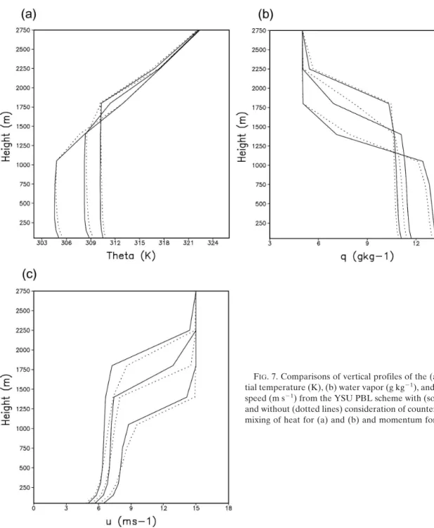
b. The role of countergradient mixing in the YSU and MRF PBL schemes

The effects of the nonlocal term for temperature and moisture,␥cin (4), are presented in Figs. 7a,b for the

YSU PBL, and Figs. 8a,b for the MRF PBL, and the nonlocal mixing of momentum in Fig. 7c for YSU PBL. Note that the countergradient mixing terms for water substances including water vaporqare not considered in the YSU PBL and the current version of the MRF PBL schemes because they are passive variables that are not necessarily correlated with the thermals. In the YSU PBL, the inclusion of countergradient mixing for moisture, that is␥qin (4), showed a negligible effect on

the PBL structure (not shown). Thus, the differences in temperature and moisture in Figs. 7 and 8 come from the nonlocal mixing effect of temperature.

For both schemes, it is clear that the nonlocal turbu-lent mixing of heat due to the countergradient effect plays a role in neutralizing the gradient by cooling the lower part of PBL and warming the upper part. In the YSU PBL, the temperature is slightly unstable in the lower part of the PBL when the countergradient mixing is not considered (Fig. 7a). Weakening of turbulent mixing for moisture is due to the lowered mixed layer height when the nonlocal heat flux is considered (Fig. 7b). The same effect appears in the MRF PBL, but with a greater magnitude in the inversion layer because the FIG. 5. Time–height cross sections of the eddy diffusivity for thermal properties (m2_s⫺1_{) calculated with the (a) YSU PBL and}

(b) MRF PBL schemes.

effect of the countergradient term in this scheme pen-etrates aboveh(Figs. 8a,b). In the MRF PBL case, the resulting temperature profiles show a stable feature, whereas the temperature is near neutral in the YSU PBL. It is evident that the effect of the nonlocal mo-mentum flux in the YSU PBL also neutralizes the wind shear (Fig. 7c). A decrease of wind speed within the PBL is discernible, except for a slight increase near the surface. This shows that the increase of winds near the surface and the decrease above in Fig. 6c is due to the countergradient mixing of momentum.

Stevens (2000) demonstrated that there is only a lim-ited range of values for the nonlocal flux in TM86 that lead to physical profiles across a reasonable range of parameter space. Also, the nonlocal flux in the MRF

PBL can be excessive, and a sharply decreasing shape ofKin the upper part of the PBL is desirable to reduce the amount of nonlocal flux (B. Stevens 2001, personal communication). Another misconception in the MRF PBL may be that the nonlocal flux penetrates up to the top of entrainment zone, whereas the effect is confined below the minimum flux level in the YSU PBL ap-proach. Having the nonlocal flux across the minimum flux level in the TM86 scheme is regarded to be a dis-advantage of the MRF PBL.

c. Further sensitivity of the parameters in the YSU PBL scheme

In addition to the nonlocal flux term due to the coun-tergradient mixing in the YSU BPL, several sensitivity

FIG. 6. Time–height evolution of the differences of the (a) potential temperature (K), (b) water vapor (g kg⫺1_{), and (c)}

wind (m s⫺1_{) resulting from the YSU PBL and MRF PBL}

schemes.

experiments are conducted to investigate the impor-tance of the parameters in the YSU PBL. Additional parameters in the YSU PBL scheme includeain (A12) and␦in (A14), where the former determines the ther-mal excess used for h, and the latter the depth of the entrainment zone.

Figure 9 shows that the impact of the perturbation temperature term in computing h is relatively large. This is because the factor ain (A12) directly controls the magnitude of turbulent mixing by determining the mixed-layer height that is defined as the minimum flux

level. By doubling the factora, the scheme works more like the MRF PBL in terms of the height of the mixed layer. On the other hand, the effect of the definition of the entrainment zone,␦in (A14), is negligible. This is because the diffusion coefficients decrease exponen-tially rapidly aboveh.

5. Real-time forecasts in the WRF model

Recently, the WRF model has been increasingly ap-plied at grid sizes of 4 km or less in real-time

cloud-FIG. 7. Comparisons of vertical profiles of the (a) poten-tial temperature (K), (b) water vapor (g kg⫺1_{), and (c) wind}

speed (m s⫺1_{) from the YSU PBL scheme with (solid lines)}

and without (dotted lines) consideration of countergradient mixing of heat for (a) and (b) and momentum for (c).

resolving forecasts. The WRF was run daily over the central United States to evaluate its usefulness as a guidance tool for forecasters participating in the Bow-Echo and Mesoscale Convective Vortex Experiment

(BAMEX; Davis et al. 2004) field program. With a 4-km grid size and no cumulus parameterization, it was found to have skill in predicting the occurrence and mode of precipitating systems in the spring of 2003. The FIG. 8. Same as in Figs. 7a,b but for the MRF PBL scheme.

FIG. 9. (a) Time–height evolution of the PBL height (m) and (b) potential temperature (K) profiles at 1400 LST, obtained from the sensitivity experiments designed in section 4c, YSU PBL (solid), and YSU PBL witha⫽13.6 in (A12) (long dashed), and witha⫽3.4 (dotted), and with the doubled (short dashed) and halved (dot–dashed) entrainment zone in (A14). Note that the solid, short-dashed, and dot–dashed lines overlap.

PBL scheme chosen for BAMEX was the YSU PBL, and part of the success must be attributed to this scheme’s capability because the forecasts were initial-ized at 0000 UTC in the local evening and run for 36 h, so that a complete diurnal cycle of PBL development was captured in the middle hours of the forecast.

Prior to BAMEX, the MRF PBL and YSU PBL were evaluated in several real-time and case studies. The most significant differences were in the developed PBL soundings in clear-sky conditions where the YSU PBL

produced lower well-mixed-layer depths, and cooler, moister PBL structures, as was expected from the re-sults in ideal case runs in the previous section. However, a few cases also showed distinct rainfall differences that can be understood in terms of the differences in these schemes. Here, one such case that exhibited significant sensitivity to PBL treatment will be presented.

a. Case description and model setup

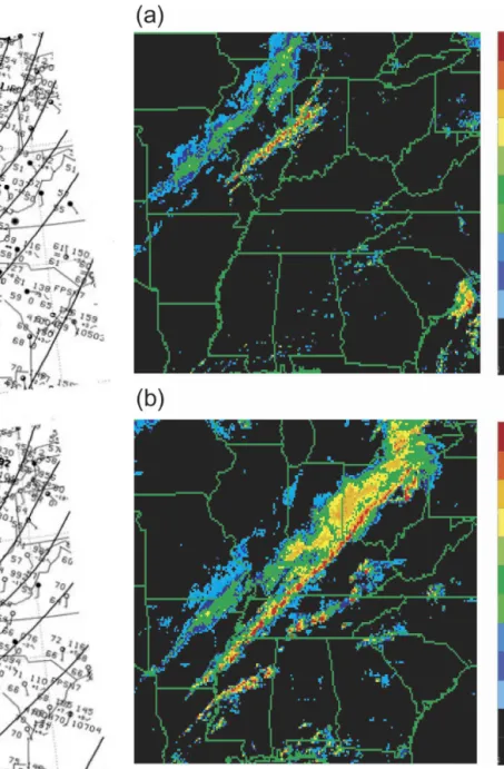
Convection triggered along a strong cold front and spawned 75 tornados in 13 states on the night of 10 November 2002. Ohio, Tennessee, and Alabama all had FIG. 10. Surface analyses for (a) 1200 UTC 10 Nov and (b) 0000

UTC 11 Nov 2002. The map is a fraction of the daily weather map issued by NCEP.

FIG. 11. Composite maximum reflectivity (dBZ) at (a) 1800

UTC 10 Nov and (b) 0000 UTC 11 Nov 2002.

SEPTEMBER2006 H O N G E T A L . 2329

numerous tornados as a 1000-km highly convective front produced a broad swath of damage resulting in 36 deaths. Tornado outbreaks of this magnitude are rare in November, but a meeting of warm moist air from the Gulf of Mexico and cold air from Canada was particu-larly abrupt and focused on this occasion. At 1200 UTC 10 November 2002 (model initial time), a surface front extended southwestward with a center in Wisconsin (Fig. 10a). A cold front had surged eastward extending from Louisiana to the northeastern United States at 0000 UTC 11 November (Fig. 10b). Between 1500 and 1800 UTC convection developed along the cold front in Illinois, and over the next 6 h lengthened into a severe convective line ahead of the front from Ohio to Ala-bama (Fig. 11).

This case was simulated with the WRF model (Ska-marock et al. 2005) on a large (380⫻380⫻34 levels) 4-km grid. Version 2.0 of the WRF was used with the Noah land surface model (Chen and Dudhia 2001), and WRF single-moment six-class microphysics (Hong et al. 2004; Hong and Lim 2006), Dudhia (1989) simple cloudinteractive shortwave, and rapid radiative transfer model longwave radiation (Mlawer et al. 1997) schemes. No cumulus parameterization was used be-cause at 4 km, updrafts may be resolved sufficiently to provide the convective vertical transports explicitly.

The simulation was initialized at 1200 UTC 10 No-vember 2002, and was run for 24 h driven by initial and 3-hourly boundary conditions from the NCEP Eta model operational forecast grids. Analyses of the simu-lation results will be focused on the first 12 h from 1200 UTC 10 November to 0000 UTC 11 November 2002, just prior to the onset of major tornado outbreaks. It was found that the simulation was more sensitive than most cases to the choice of PBL scheme. Here we will outline the differences between the simulations and ex-plain them in terms of the differences between the MRF PBL and YSU PBL. This gives us insight into potential benefits of the YSU PBL scheme in a high-resolution numerical weather prediction application.

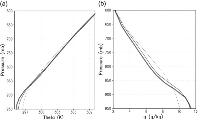
b. Results

Figure 12 compares the potential temperature and specific humidity profiles at 1800 UTC. In the tempera-ture profiles, temperatempera-tures colder below 870 mb and warmer up to 700 mb are simulated by the YSU PBL compared with the MRF PBL scheme, which is closer to the observed. This indicates that a typical afternoon cold bias at 850 mb with the MRF PBL scheme is im-proved when the YSU PBL is employed. This behavior can be explained by a direct impact of the different nature of mixing between these schemes. The impact is FIG. 12. Comparisons of boundary layer profiles of (a) potential temperature (K) and (b) specific humidity (g kg⫺1_{) at 1800 UTC 10}

Nov 2002, obtained from the analysis (thick gray), and the experiments with the YSU PBL (solid), and MRF PBL (dotted) schemes, averaged over the model domain.

more significant for the moisture. Drying near the sur-face is as large as 1.5 g kg⫺1 when the MRF PBL scheme is employed. Overall weakening of the bound-ary layer mixing with the YSU PBL is due to the syn-optic situations accompanying relatively strong winds embedded within a cold front. This point will be further explained later.

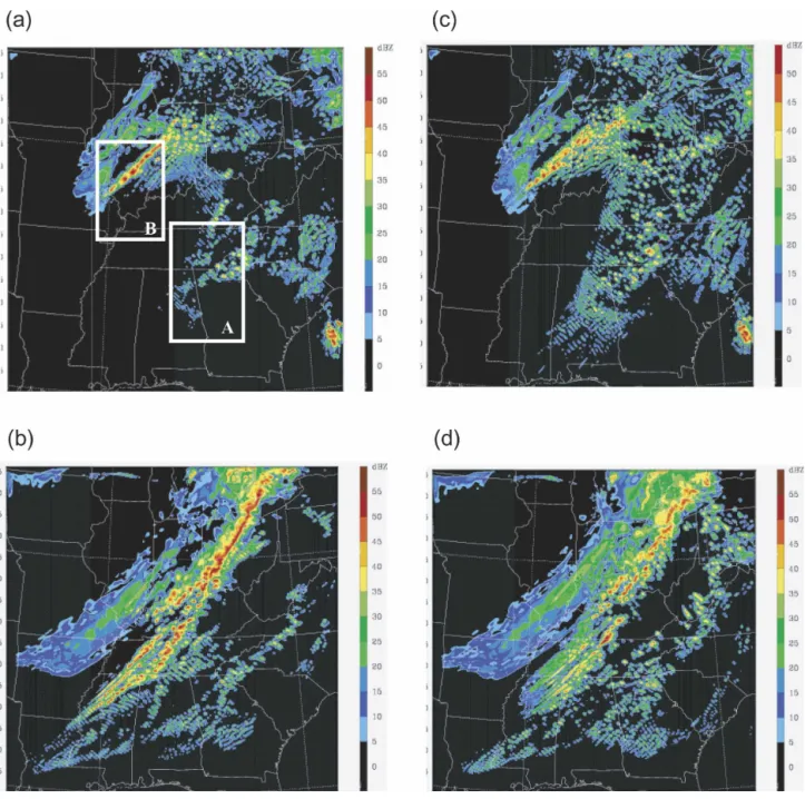
It is apparent that the simulation with the YSU PBL scheme intensified the front more rapidly and length-ened the line of severe convection, in better agreement

with observations, than the MRF PBL (see Fig. 13). Figure 13b compared with Fig. 11b also shows that some characteristics, such as a double line of intense convection at 0000 UTC were captured to some extent in the YSU PBL simulation, while comparing Fig. 13d shows that the MRF PBL line extension to the south was weaker than observed at this time. On the other hand, it is distinct that the YSU PBL scheme reduces spurious widespread convection in front of intense con-vection regions that is seen in the simulation with the FIG. 13. Simulated maximum reflectivity (dBZ) with YSU PBL at (a) 1800 UTC 10 Nov and (b) 0000 UTC 11 Nov 2002, and (c), (d) the corresponding forecasts with MRF PBL. The boxes A and B designate the light and heavy precipitation regions, respectively, for time variations analyses in Figs. 16–18.

SEPTEMBER2006 H O N G E T A L . 2331

MRF scheme, in particular at 1800 UTC (cf. Figs. 11a and 13a,c).

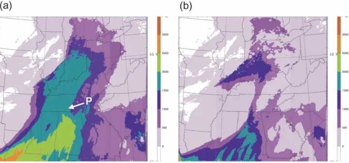
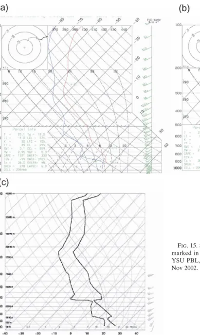
The reason for the 0000 UTC intensity difference can be inferred by comparing the prefrontal CAPE at 1800 UTC (Fig. 14). The YSU PBL shows a large region of significantly higher CAPE where convection later de-velops when triggered by the front. It was during this development phase that the PBL scheme sensitivity be-came most apparent. A typical sounding from Tennes-see (Fig. 15) shows a significant difference in the PBL depth in this case. This difference is more exaggerated here than in most other situations, but it shows that the shallower moister PBL produced by the YSU scheme has more CAPE than the deeper drier MRF PBL. An observed 1800 UTC sounding from Nashville, Tennes-see, shows that the YSU PBL captured the PBL depth much better, but there is a difference in the strengths of the inversions in the observed and modeled soundings. The lack of definition in the upper inversion at the 625-mb level may be due to overactive free atmospheric diffusion, and/or due to insufficient vertical resolution that is about 30 mb.

A large region of significantly higher CAPE is due to the reduced entrainment of dry air into the PBL during the morning hours, which is a direct result of the en-trainment parameterization of the YSU PBL, as seen from the idealized experiments in the previous section. In this case the MRF PBL is particularly active because of a strong 20 m s⫺1_{southwesterly flow just above the}

boundary layer, which leads to a decrease of the PBL’s Rib used to compute the boundary layer height, and

hence enhances the entrainment above the inversion layer. In the YSU PBL scheme, the shear only contrib-utes in a secondary way to enhance entrainment, which is mostly governed by the magnitude of the surface fluxes, and thus does not maximize until later in the day.

Despite the higher CAPE with the YSU PBL com-pared with the MRF PBL, the radar reflectivity in Fig. 11 showed the weakening of convection in the prefron-tal region. The reason can be better explained by ex-amining the frontal and prefrontal regions separately. It is seen that the light precipitation in front of intense convection is better captured by the YSU PBL than the MRF PBL, although the there is a difference in diurnal variation of the precipitation (Fig. 16a). In the intense convection region, the model generally underestimated the precipitation amount irrespective of the choice of the PBL scheme, but the YSU PBL scheme better cap-tured the time variation of the precipitation associated with late afternoon convection after 210 UTC 10 No-vember 2002 (Fig. 16b).

The reason for the precipitation and reflectivity dif-ferences can be inferred by comparing the relative hu-midity and temperature profiles that are directly af-fected by the vertical turbulent mixing. Moistening within the PBL and drying above due to weaker mixing by the YSU PBL than the MRF PBL appear in both light and intense convection regions (Fig. 17). Tem-perature difference follows the same behavior as in the moisture, but with the opposite signs (not shown). Cooling below the PBL top and warming above it were FIG. 14. Simulated CAPE at 1800 UTC 10 Nov 2002 with (a) YSU PBL and (b) MRF PBL. The station point P in (a) is the place

for the sounding analysis in Fig. 15.

2332 M O N T H L Y W E A T H E R R E V I E W VOLUME134

apparent in both regions. These behaviors of the YSU PBL scheme reflect the improved PBL structure includ-ing the inversion in front of a cold front (see also Fig. 15).

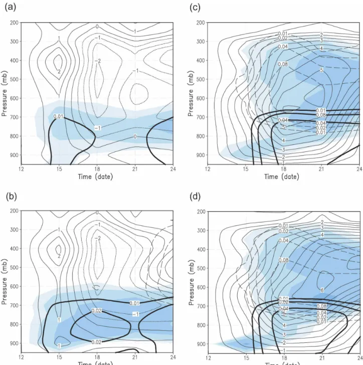
A typical difference in the thermodynamical struc-ture of the PBL between the two schemes induces weakened (strengthened) convection activities in pre-frontal (pre-frontal) regions as seen in Fig. 13. To illustrate the difference in the predicted convection, we compare the temporal evolution of the vertical velocity and hy-drometeors simulated by the MRF PBL and YSU PBL (Fig. 18). In the prefrontal region (Figs. 18a,b), warm clouds are dominant. Downward motion is prevalent above the PBL in the daytime when the PBL develops,

indicating the formation of the inversion layer at the PBL top (as seen in Fig. 15). This inversion inhibits the initiation of convection. Both the YSU and MRF PBL schemes show the development of clouds in the morn-ing hours, but more actively in case of the MRF PBL scheme. This is because the intensity of the inversion layer is strong with the YSU PBL scheme, which leads to a weakening of the vertical motion within the PBL. The relative humidity in cloud layers is also smaller with the YSU PBL than with the MRF PBL (see Fig. 17a). Consequently, the YSU PBL scheme produces less early cloud activity, although the CAPE is larger.

The same scenario applies to the intense convection region in terms of the mixing properties due to the FIG. 15. Simulated sounding near Nashville, TN, at the point P marked in Fig. 14a, obtained from the experiments with the (a) YSU PBL, (b) MRF PBL, and (c) the observed at 1800 UTC 10 Nov 2002.

SEPTEMBER2006 H O N G E T A L . 2333

different PBL schemes. Moistening and cooling within the PBL and drying and warming above the PBL top are also significant in the intense convection region (Fig. 17b), but the impact on the predicted convection is different from the case of weak convection in the pre-frontal region. The reason can be attributed to the

dif-ferences in synoptic environment associated with the formation of convection (Figs. 18c,d). Upward motion prevails within the entire troposphere and cloud tops reach the tropopause, whereas the downward motion is dominant above the PBL ahead of a front. Ice micro-physics is the key mechanism, whereas warm clouds are

FIG. 17. Time variation of the differences in relative humidity (%) (YSU PBL minus MRF PBL experiments) from 1200 UTC 10 Nov to 0000 UTC 11 Nov 2002 averaged over the (a) light and (b) heavy precipitation regions, marked A and B in Fig. 13a, respectively.

FIG. 16. Time variation of 3-h accumulated precipitation from 1500 UTC 10 Nov to 0000 UTC 11 Nov 2002 obtained from the observation (thick gray), YSU PBL (solid), and MRF PBL (dotted) runs, averaged over the (a) light and (b) heavy precipitation regions, marked A and B in Fig. 13a, respectively. The observed precipitation from the stage-IV data with a 4-km grid is interpolated to the model grid. [Available online at http://www.emc.ncep.noaa.gov/mmb/ylin/pcpanl/.]

dominant in the prefrontal region. This indicates that, in contrast to the prefrontal region, the PBL processes play a secondary role in the intense convection region. Because of the weakened mixing in the YSU PBL, the PBL clouds are weakened before 2100 UTC 10 Novem-ber, but with negligible difference. Because the synop-tic environment associated with the frontal convection

is strong, the difference in the PBL mixing does not influence the overall evolution of daytime convection. The enhanced convection in late afternoon in case of the YSU PBL is due to the moister boundary layer below clouds, which leads to a reduced evaporation of falling precipitation. The 3-h accumulated precipitation ending 0000 UTC 11 November is nearly doubled (see FIG. 18. Time variation of the vertical velocity [cm s⫺1_{; upward (solid) and downward (dotted)], cloud and ice water (shaded),}

rainwater (g kg⫺1_{, thick solid), snow and graupel (long dashed) from 1200 UTC 10 Nov to 0000 UTC 11 Nov 2002, obtained from the}

(a) YSU PBL and (b) MRF PBL experiments, averaged over the light precipitation region (marked A in Fig. 13a), and (c), (d), over the heavy precipitation region (marked B in Fig. 13a). Contour lines and shaded intensity are at 0.01, 0.02, 0.04, and 0.08 g kg⫺1_.

SEPTEMBER2006 H O N G E T A L . 2335

Fig. 16b). The overall resulting impact is that the boundary layer from the YSU PBL scheme remains less diluted by entrainment leaving more fuel for severe convection when the front triggers it.

6. Concluding remarks

In this paper, we have proposed a revised vertical diffusion package with a nonlocal turbulent mixing in the PBL that is suitable for weather forecasting and climate models. Significant revisions are introduced to the MRF PBL (HP96) that was based on the nonlocal diffusion concept of TM86. The major ingredient of the modifications is the inclusion of an explicit treatment of the entrainment processes at the top of PBL proposed by N03, whereas it is treated implicitly in the MRF PBL by raising the PBL height. The new diffusion package is named the YSU PBL. A comprehensive description of the new package has been given, and its characteristics were examined in a one-dimensional offline test frame-work as well as real-time forecasts in the WRF model. It is found that the YSU PBL scheme produces a realistic structure of the PBL in response to an ideal-ized daytime variation of surface heat and moisture fluxes. The vertical resolution dependency of the new algorithm is acceptable. Compared with the MRF PBL scheme, the YSU PBL increases boundary layer mixing in the thermally induced free convection regime and decreases it in the mechanically induced forced convec-tion regime, which alleviates the well-known problems in the MRF PBL. The problem of early development of the PBL before noon is also resolved. Improvements are due to the explicit specification of the entrainment at the inversion layer by removing the ambiguity of treating it as a component of the MRF PBL’s internal eddy mixing. In the YSU PBL, the magnitude of the nonlocal mixing term is smaller than that of the MRF PBL, and plays a role in neutralizing the PBL structure whereas the nonlocal flux in the MRF PBL produces an overstable structure. It is found that the specification of the boundary layer height, using a smaller thermal ex-cess and a zero critical bulk Richardson number, is very important in the YSU PBL because it determines the minimum flux level.

The performance of the YSU PBL scheme in a case study with the WRF model showed that the new scheme improves the representation of the boundary layer in such a way that an advancing cold front more realistically triggers the convection that occurs later in the day. In the frontal region the YSU PBL scheme improves some characteristics, such as a double line of intense convection. This is because the YSU PBL scheme remains less diluted by entrainment leaving

more fuel for severe convection when the front triggers it. The new scheme does a better job in reproducing the convective inhibition in the prefrontal region. Because the convective inhibition is accurately predicted, the widespread light precipitation ahead of a front, in the case of the MRF PBL, is reduced, supporting the idea that the YSU PBL is more physically based in repre-senting the PBL-top entrainment explicitly rather than it implicitly.

The results presented here show that the new scheme is a promising option in mesoscale models alleviating several problems inherent in its predecessor (the MRF PBL). The enhancements to the YSU PBL scheme have little impact on its efficiency, making it a viable option for real-time forecasting and computer-intensive regional climate runs. Since its addition in the WRF, it has been used regularly in real-time forecasts at NCAR, including hurricane forecasts and has proved to be robust and realistic in its behavior in a wide variety of situations since its first inclusion in 2003. Systematic verifications were carried out as part of the Develop-mental Test Bed Center’s Retrospective Test Plan (Bernadet et al. 2005) in several high-resolution win-dow domains for monthlong periods over the United States, and also included the YSU PBL in the Ad-vanced Research WRF and in the NCEP Nonhydro-static Mesoscale Model in some ensemble members. These results, along with the value of WRF in BAMEX (Davis et al. 2004) demonstrated that the new scheme is a competitive choice for current-day models.

Acknowledgments.This work was funded by the Ko-rea Meteorological Administration Research and De-velopment Program under Grant CATER-2006-2204. A part of this work was done during the first author’s (S-Y. Hong) visit to NCAR, which was partly sup-ported by NCAR. We are grateful to Tae-Young Lee, John Brown, and Joe Klemp for their interest and en-couragement.

APPENDIX A

The Revised Vertical Diffusion Scheme

a. Mixed-layer diffusion

As in TM86, HP96, and N03, the momentum diffu-sivity coefficient is formulated as

Km⫽kwsz

冉

1⫺

z h

冊

p

, 共A1兲

wherepis the profile shape exponent taken to be 2,k

is the von Kármán constant (⫽0.4),zis the height from

the surface, andhis the height of the PBL. The mixed-layer velocity scale is represented as

ws⫽共u 3 *⫹␾mkw 3 *bzⲐh兲 1Ⲑ3_{, 共A2兲}

whereu_*is the surface frictional velocity scale, and␾m

is the wind profile function evaluated at the top of the surface layer, and the convective velocity scale for the moist air, w

*b⫽ [(g/␪␷a)(w⬘␪⬘␷)0h]

1/3_{. The}

countergra-dient term for ␪and momentum is given by

␥c⫽b

共w⬘c⬘兲0

ws0h

, 共A3兲

where (w⬘c⬘)0is the corresponding surface flux for␪,u,

and ␷, and bis a coefficient of proportionality, which will be derived below. Note that the countergradient mixing terms for water substances including water va-porqare not considered. In other words, the potential temperature and horizontal velocity components are the only variables for nonlocal term due to the coun-tergradient mixing [␥_␪in (4)]. The mixed-layer velocity scalews0in (A3) is defined as the velocity atz⫽0.5h

in (A2).

The eddy diffusivity for temperature and moistureKt

is computed fromKmin (A1) by using the relationship

of the Prandtl number of N03, which is given by Pr⫽1⫹共Pr0⫺1兲exp关⫺3共z⫺␧h兲

2_Ⲑh2

兴, 共A4兲 where Pr0, (␾t/␾m⫹bk␧), is the Prandtl number at the

top of the surface layer given by TM86 and HP96. The ratio of the surface layer height to the PBL height,␧, is specified to be 0.1. In (A4) Pr increases upward rather than being a constant within the whole mixed boundary layer as in TM86 and HP96.

To satisfy the compatibility between the surface layer top and the bottom of the PBL, identical profile func-tions are used to those in surface layer physics. First, for unstable and neutral conditions [(w⬘␪⬘_␷)0ⱖ0],

␾m⫽

冉

1⫺16

0.1h L

冊

⫺1Ⲑ4

for u and ␷, and

␾t⫽

冉

1⫺16

0.1h L

冊

⫺1Ⲑ2

for ␪ and q, 共A5兲 while for the stable regime [(w⬘␪⬘_␷)0⬍0],

␾m⫽␾t⫽

冋

1⫹5

0.1h

L

册

, 共A6兲

wherehis, again, the boundary layer height, and Lis the Monin–Obukhov length scale. To determine the factorbin (A3), the exponent of⫺1_{⁄3is chosen to}

en-sure the free convection limit. TypicallyLranges from

⫺50 to 0 in unstable situations. Therefore, we can use the following approximation:

␾m⫽

冉

1⫺16 0.1h L

冊

⫺1Ⲑ4 ⬇

冉

1⫺80.1h L

冊

⫺1Ⲑ3 . 共A7兲 Note that the approximated value of 12 in HP96 instead of 8 in (A7) is not correct. Following N03 and Moeng and Sullivan (1994), the heat flux amount at the inver-sion layer is expressed by

共w⬘␪⬘兲h⫽ ⫺e1wm 3 _Ⲑh

, 共A8兲

wheree1is the dimensional coefficient (⫽4.5 m⫺ 1_s2_K),

wmis the velocity scale based on the surface layer

tur-bulence (w3 m⫽w

3

*⫹5u

3

*), and the mixed-layer velocity scale for the dry airw

* ⫽[(g/␪a)(w⬘␪⬘0)h]

1/3_{. Using a}

typical value of␪at 300 K, the gravity at 10 m s⫺2_{, and}

the limit ofu

*⫽0 in the free convection limit, (A8) can be generalized for the moist air with a nondimensional constant, which can be expressed by

共w⬘␪⬘_␷兲h⫽ ⫺0.15

冉

␪␷a

g

冊

wm

3 _Ⲑh

, 共A9兲

wherewmconsiders the water vapor driven virtual

ef-fect for buoyancy flux. Equation (A9) implies that the entrainment flux is ⫺0.15 times the surface flux of buoyancy, which is a standard finding in LES. Given the buoyancy flux at the inversion layer [(A9)], the flux at the inversion layer for scalars ␪ and q, and vector quantitiesuand␷,is proportional to the jump of each variable at the inversion layer:

共w⬘␪⬘兲h⫽we⌬␪|h, 共A10a兲

共w⬘q⬘兲h⫽we⌬q|h, 共A10b兲

共w⬘u⬘兲h⫽Prhwe⌬u|h, and 共A10c兲

共w⬘␷⬘兲h⫽Prhwe⌬␷|h, 共A10d兲

respectively. Here, we is the entrainment rate at the

inversion layer, which can be expressed by

we⫽

共w⬘␪⬘_␷兲h

⌬␪␷|h

, 共A11兲

where the maximum magnitude ofweis limited towmto

prevent excessively strong entrainment in the presence of too small of a jump in␪_␷ in the denominator. The Prandtl number at the inversion layer Prh, is set as 1,

which follows the asymptotic limit of Pr in (A4). The Prh ⫽0.5 from N03 occasionally produces a jump of

momentum flux, which results in numerical instability when the wind is strong near the surface. Meanwhile, the flux for the liquid water substance at the inversion layer is assumed to be zero.

In this study, following HP96 [see (1) in this paper]h

is determined as the first neutral level by checking the stability between the lowest model level and levels above considering the temperature perturbation due to surface buoyancy flux, which can be expressed by,

␪␷共h兲⫽␪␷a⫹␪T

冋

⫽a

共w⬘␪⬘_␷兲0

ws0

册

, 共A12兲

where the␪_␷(h) is the virtual potential temperature ath.

The above formula is the same as that of HP96, but the thermal excess term␪Tis smaller than that in the HP96

because of a largerws0. As shown in section 4,ais an

important parameter in the new scheme. We set the parametera⫽6.8, which is the same as thebfactor in (A3). In (A12)␪Tranges less than 1 K under clear-sky

conditions.

Numerically, h is obtained by two steps. First, h is estimated by (1) without considering␪T. This estimated

his utilized to compute the profile functions in (A5)– (A7), and to compute thews0, which is estimated to be

the value atz⫽h/2 in (A2). Usingws0and␪Tin (2),h

is enhanced. The enhancedhis determined by checking the bulk stability between the surface layer (lowest model level) and levels above. The computed bulk Ri-chardson number Rib between the surface layer and a level zis compared with Ribcr(⫽0.0). The value of h

corresponding to Ribcris obtained by linear

interpola-tion between the two adjacent model levels. With the enhanced handws0,Kmis obtained by (A1),

entrain-ment terms in (A9)–(A11), andKtby the Prandtl

num-ber in (A4). The countergradient correction terms for␪ in (4) are also obtained by (A3).

b. Free atmosphere diffusion

The local diffusion scheme, the so-called localK ap-proach (Louis 1979) is utilized for free atmospheric dif-fusion above the mixed layer (z ⬎ h). On the other hand, N03 considers the entrainment flux aboveh. The former considers the local instability of the environ-mental profile, whereas the latter expresses the pen-etration of entrainment flux abovehirrespective of lo-cal stability. We consider both effects within the en-trainment zone and the localKapproach above.

First, N03 assumes that fluxes decrease exponentially abovehwhere the diffusion coefficients for mass(t;␪, q) and momentum(m; u,␷) can be expressed by

Kt_ent⫽ ⫺共w⬘␪⬘_␷兲h 共⭸␪␷Ⲑ⭸z兲h exp

冋

⫺共z⫺h兲 2 ␦2

册

, 共A13a兲 Km_ent⫽Prh ⫺共w⬘␪⬘_␷兲h 共⭸␪␷Ⲑ⭸z兲h exp

冋

⫺共z⫺h兲 2 ␦2

册

, 共A13b兲

and where the thickness of the entrainment zone can be estimated as

␦Ⲑh⫽d1⫹d2Ricon⫺ 1

, 共A14兲

wherewmis the velocity scale for the entrainment, Ricon

is the convective Richardson number at the inversion layer {⫽[(g/␪_␷a)h⌬␪v_ent] /w

2

m}, and d1 and d2 are

con-stants, which are set as 0.02 and 0.05, respectively. Here,⌬␪v_entis the jump of the virtual potential

tem-perature across the inversion layer, which is the same as

⌬␪␷|hin (A11) by definition, but practically differ from

each other as follows. In (A11)⌬␪_␷|his the actual

dif-ference of the virtual potential temperature between the adjacent model levels across h, which is used to compute the entrainment flux in (A10), whereas here

⌬␪v_ent is the jump of ⌬␪␷ within the inversion layer.

Note that the penetration depth in (A14) is based on the theoretical formula from observations and LES data, in which the inversion layer depth is accurately determined. Because the inversion layer depth is not explicitly resolved in coarse-resolution models, we set

⌬␪v_entas a function ofh(⫽0.001h). As will be shown in

the next section, the scheme is insensitive to the mag-nitude of␦.

As in HP96, we also compute the vertical diffusivity coefficients for momentum (m; u,␷) and mass (t;␪, q), following Louis (1979) above h, and these are repre-sented by Km_loc,t_loc⫽l 2 fm,t共Rig兲

冉

⭸U ⭸z

冊

共A15兲

in terms of the mixing lengthl, the stability functions

fm,t(Rig), and the vertical wind shear,|⳵U/⳵z|. The

sta-bility functionsfm,tare represented in terms of the local

gradient Richardson number Rig. For the noncloudy layer,

Rig⫽g

␪␷

冋

⭸␪␷Ⲑ⭸z

共⭸UⲐ⭸z兲2

册

. 共A16a兲

For the cloudy air, Rig is modified for reduced stability within cloudy air, which can be expressed by

Rigc⫽

冉

1⫹ L_␷q_␷ RdT

冊

冋

Rig⫺ g 2 |⭸UⲐ⭸z|2 1 CpT 共A⫺B兲 共1⫹A兲

册

, 共A16b兲 whereA⫽L2 ␷q␷/CpR␷T2andB⫽L␷q␷/RdT. Equation

(A16b) is adapted from Durran and Klemp (1982). For cloudy air, Rig in (A16a) is replaced by Rigcin (A16b)

in computing (A15). The computed Rig is bounded to

⫺100 to prevent unrealistically unstable regimes. The mixing length scalelis given by

1 l⫽ 1 kz⫹ 1 ␭0 , 共A17兲

where k is the von Kármán constant (⫽0.4), z is the height from the surface. Here ␭0 is the asymptotic

length scale (⫽150 m), which is based on Kim and Mahrt (1992).

The stability functionsfm,t(Rig) differ for stable and

unstable regimes. We adopt the stability formulas used in the NCEP MRF model (Betts et al. 1996). For the stably stratified free atmosphere (Rig⬎0),

ft共Rig兲⫽

1

共1⫹5Rig兲2 共A18兲 and the Prandtl number is given by

Pr⫽1.0⫹2.1⫽Rig. 共A19兲 For the neutral and unstably stratified atmosphere (Rigⱕ0),

ft共Rig兲⫽1⫺

8Rig

共1⫹1.286

公

⫺Rig兲 and 共A20a兲

fm共Rig兲⫽1⫺

8Rig

共1⫹1.746

公

⫺Rig兲. 共A20b兲 For the entrainment zone aboveh, the diffusivity is determined by geometrically averaging the two differ-ent diffusivity coefficidiffer-ents from (A13) and (A15), and is expressed by

Km,t⫽共Km,t_entKm,t_loc兲 1Ⲑ2

. 共A21兲

The top of the entrainment zone is determined as the level at which 1% of the minimum flux at hexists, in which the value of the exponential terms in (A13) is 4.6. Note that (A21) represents not only the entrainment

but also the free atmospheric mixing when the entrain-ment above the bottom of the inversion layer is induced by vertical wind shear at PBL top. Above the entrain-ment zone, the local approach is then used, Km,t ⫽

Km,t_loc.

We also introduce a small background diffusion (0.001 times the vertical grid length) so that the com-puted Kz is bounded between this and 1000 m

2_s⫺1_.

Here Pr is set between 0.25 and 4.0. With the diffusion coefficients and countergradient correction terms com-puted in (A1)–(A21), the diffusion equations for all prognostic variables, (4), are solved by an implicit nu-merical method, as described in appendix B.

APPENDIX B

Numerical Method of Solution

The numerical formulation as applied to the poten-tial temperature equation is discussed here. The ar-rangement and nomenclature of layers is as shown in Fig. B1.

The diffusion equation for potential temperature in (4) is given by ⭸␪ ⭸t⫽ ⭸ ⭸z

冋

Kt

冉

⭸␪ ⭸z⫺␥T

冊

⫺共w⬘␪⬘兲h

冉

z h

冊

3

册

. 共B1兲 The finite-difference centered-in-zform of (B1) is

␪k n⫹1 ⫺␪k n⫺1 2⌬t ⫽ 1 ⌬Zk

冋

Kk ⌬Zˆk 共␪k⫹1 n⫹1_⫺␪ k n⫹1_⫹⌬Zˆ k␣兲 ⫺ Kk⫺1 ⌬Zˆ k⫺1 共␪k n⫹1_⫺␪ k⫺1 n⫹1_⫹⌬Zˆ k⫺1␣兲

册

, 共B2兲 where␣ ⫽ 关⫺␥T⫺(w⬘␪⬘)h(z/h) 3 K⫺t1]. The subscripttis

omitted in the diffusion coefficient hereafter.

FIG. B1.The arrangement and nomenclature of layers for the numerical formulation applied to the potential temperature equation described in appendix B.

And we define, ␥k⫺1⫽ 2⌬tKk⫺1 ⌬Zˆ k⫺1 1 ⌬Zk , ␦k⫽ 2⌬tKk ⌬Zˆ k 1 ⌬Zk , and ␮k⫽␣⌬Zˆk. 共B3兲

The general interior equation, for 1⬍k⬍kxhas the form ␪k n⫹1_⫽␪ k n⫺1_⫹␦ k共␪k⫹1 n⫹1_⫺␪ k n⫹1_兲⫹␦ k␮k ⫺␥k⫺1共␪k n⫹1_⫺␪ k⫺1 n⫹1 兲⫺␥k⫺1␮k⫺1. 共B4兲

For the top layer, k ⫽ kx the boundary condition is

K(⳵␪/⳵Z)⫽0, so the equation becomes

␪kx n⫹1_⫺␪ kx n⫺1 2⌬t ⫽ 1 ⌬Zkx

冋

0⫺ Kkx⫺1 ⌬Zˆkx⫺1 共␪kx n⫹1 ⫺␪kx⫺1 n⫹1 ⫹⌬Zˆ kx⫺1␣兲

册

. 共B5兲

The lower boundary condition is

K1

冉

⭸␪ ⭸Z

冊

⫽ ⫺ H0 ␳Cp ⫽ ⫺共w⬘␪⬘兲0, 共B6兲

which is passed from the land surface model. The equation for the lowest layerk⫽1 is now

␪1 n⫹1_⫺␪ 1 n⫺1 2⌬t ⫽ 1 ⌬Z1

冋

K1 ⌬Zˆ1 共␪2 n⫹1_⫺␪ 1 n⫹1_⫹␣⌬ Zˆ1兲 ⫹H0Ⲑ共␳Cp兲

册

共B7兲

and the upper and lower boundary equations now be-come ␪kx n⫹1_⫽␪ kx n⫺1_⫺␥ kx⫺1共␪kx n⫹1_⫺␪ kx⫺1 n⫹1 _兲 ⫺␥kx⫺1␮kx⫺1, and ␪1 n⫹1_⫽␪ 1 n⫺1_⫺␦ 1共␪2 n⫹1_⫺␪ 1 n⫹1 兲⫺␦1␮1⫹␤, 共B8兲

respectively, where ␤ ⫽ 2⌬tH0/⌬Z1␳Cp.

Recombina-tion of terms yields, for interior, top, and bottom:

⫺␥k⫺1␪k⫺1 n⫹1_{⫹共1⫹␦} k⫹␥k⫺1兲␪k n⫹1_⫺␦ k␪k⫹1 n⫹1 ⫽␪k n⫺1_⫹␦ k␮k⫺␥k⫺1␮k⫺1, ⫺␥kx⫺1␪kx⫺1 n⫹1 ⫹共1⫹␥kx⫺1兲␪kx n⫺1 ⫽␪kx n⫺1_⫺␥ k⫺1␮kx⫺1, and 共1⫹␦1兲␪1 n⫹1_⫺␦ 1␪2 n⫹1_⫽␪ 1 n⫺1_⫹␦ 1␮1⫹␤, 共B9兲

respectively. Equation (B9) can be expressed in a tridi-agonal matrix (A␪⫽F), and is given by

冢

1⫹␦1 ⫺␦1 0 0 ⫺␥1 1⫹␦2⫹␥1 ⫺␦2 0 · · · · 0 0 ⫺␥kx⫺1 1⫹␥kx⫺1

冣冢

␪1 ␪2 · · · ␪kx

冣

n⫹1 ⫽

冢

␪1 n⫺1_⫹␦ 1␮1⫹␤ ␪2 n⫺1_⫹␦ 2␮2⫺␥1␮1 · · · ␪kx n⫺1_⫺␥ kx⫺1␮kx⫺1

冣

, 共B10兲

where the main diagonals ofAare defined as AD共k兲⫽共1⫹␦k⫹␥k⫺1兲,

AD共1兲⫽共1⫹␦1兲, and

AD共kx兲⫽共1⫹␥kx⫺1兲, 共B11兲

and the upper and lower diagonals are AU共k兲⫽ ⫺␦k and

AL共k兲⫽ ⫺␥k⫺1. 共B12兲

The vector of potential temperature␪is solved using the matrixAand forcingFin subroutine TRIDIN.

REFERENCES

Ayotte, K. W., and Coauthors, 1995: An evaluation of neutral and convectively planetary boundary layer parameterizations relative to large eddy simulations.Bound.-Layer Meteor.,79, 131–175.

Basu, S., G. R. Iyengar, and A. K. Mitra, 2002: Impact of a non-local closure scheme in a simulation of a monsoon system over India.Mon. Wea. Rev.,130,161–170.

Bernardet, L. R., L. B. Nance, H.-Y. Chuang, A. Loughe, M. Demirtas, S. Koch, and R. Gall, 2005: The Developmental Testbed Center Winter Forecasting Experiment. Preprints,

21st Conf. on Weather Analysis and Forecasting/17th Conf. on Numerical Weather Prediction,Washington, DC, Amer. Me-teor. Soc., CD-ROM, P7.1.

Betts, A., S.-Y. Hong, and H.-L. Pan, 1996: Comparison of NCEP–NCAR reanalysis with 1987 FIFE data.Mon. Wea. Rev.,124,1480–1498.

Braun, S. A., and W.-K. Tao, 2000: Sensitivity of high-resolution simulations of Hurricane Bob (1991) to planetary boundary layer parameterizations.Mon. Wea. Rev.,128,3941–3961. Bright, D. R., and S. L. Mullen, 2002: The sensitivity of the

nu-merical simulation of the southwest monsoon boundary layer to the choice of PBL turbulence parameterization in MM5.

Wea. Forecasting,17,99–114.

Caplan, P., J. Derber, W. Gemmill, S.-Y. Hong, H.-L. Pan, and D. Parrish, 1997: Changes to the 1995 NCEP operational me-dium-range forecast model analysis-forecast system. Wea. Forecasting,12,581–594.

Chen, F., and J. Dudhia, 2001: Coupling an advanced land sur-face–hydrology model with the Penn State–NCAR MM5