Forecasting and Information Sharing in Supply Chains Under
Quasi-ARMA Demand
Avi Giloni∗, Clifford Hurvich †, Sridhar Seshadri‡
July 9, 2009
Abstract
In this paper, we revisit the problem of demand propagation in a multi-stage supply chain in which the retailer observes ARMA demand. In contrast to previous work, we show how each player constructs the order based upon its best linear forecast of leadtime demand given its available information. In order to characterize how demand propagates through the supply chain we construct a new process which we call quasi-ARMA or QUARMA. QUARMA is a generalization of the ARMA model. We show that the typical player observes QUARMA demand and places orders that are also QUARMA. Thus, the demand propagation model is QUARMA-in-QUARMA-out. We study the value of information sharing between adjacent players in the supply chain. We demonstrate that under certain conditions information sharing can have unbounded benefits. Our analysis hence reverses and sharpens several previous results in the literature involving information sharing and also opens up many questions for future research.
KEYWORDS: Supply Chain Management, Information Sharing, Time Series, ARMA, Invert-ibility.
∗Sy Syms School of Business, Yeshiva University, BH-428, 500 West 185th St., New York, NY 10033. E-mail: [email protected]
†Department of Information, Operations, and Management Science, Leonard N. Stern School of Business, New
York University, Suite 8-52, 44 West 4th St., New York, NY 10012. E-mail: [email protected] ‡IROM B6500, 1 University Station, Austin, TX 78712. E-mail: [email protected]
1
Introduction
We study demand propagation in a multi-stage supply chain in which the retailer observes ARMA demand with Gaussian white noise (shocks). Similar to previous research, we assume each supply chain player constructs a linear forecast for the leadtime demand and uses it to determine the order quantity via a periodic review myopic order-up-to policy. The new feature in our paper is the derivation of thebest linear forecast of leadtime demand for each supply chain player given the particular information that is available to that player. This is important since under the assumption of Gaussian white noise the best linear forecast is the best forecast. Therefore, in the absence of the best linear forecast, the order quantity determined by a player would be sub-optimal, see for example Johnson and Thompson (1975).
In order to construct its best linear forecast, we describe how a supply chain player must first, via a traditional time-series methodology, characterize the information available to the player. We assume that information sharing occurs only between contiguous players. We show that under certain assumptions there arise only four mutually exclusive and exhaustive information sets when contiguous players either share or do not share their information (shocks). This permits us to exactly construct a recursive process that characterizes how demand propagates from player to player when each player uses his or her best linear forecast. Under each of the four information sets, we show that the demand propagation model is QUARMA-in-QUARMA-out where a QUARMA model is defined in (3) and is a more general time series model than an ARMA model. This result generalizes the ARMA-in-ARMA-out property proposed by Zhang (2004). Furthermore, we show that under certain conditions information sharing can have tremendous benefits. Our analysis hence reverses and sharpens several of the previous results in the literature involving information sharing and also opens up many questions for future research.
Our paper is an extension of the work of Lee, So and Tang (2000) and Raghunathan (2001), Zhang (2004) and Gaur, Giloni, and Seshadri (GGS, 2005), who study the value of information
sharing in supply chains. Zhang and GGS extend the original work of Lee, So and Tang (2000) and Raghunathan (2001) by studying the value of information sharing in supply chains where the retailer serves an ARMA(p,q) demand as opposed to AR(1) demand. In each of these papers, the
retailer places orders with a supplier using a periodic review order-up-to policy. Both the supplier and the retailer know the parameters of the demand process, however, the retailer may or may not choose to share information about the actual realizations of demand with the supplier. Zhang (2004) studies how the order process propagates upstream in a supply chain under the assumption that ARMA demand to the retailer is invertible. Zhang does not consider the case when demand becomes non-invertible at any stage of the chain, a phenomenon that GGS point out can happen even though the retailer’s demand is invertible.
The concept of invertibility is central to an understanding of the value of information shar-ing, and also to an understanding of how demand propagates through a supply chain. In any ARMA(p, q) model for demand at a given stage of the supply chain, a linear combination of the
present observation andppast demand observations is set equal to a constant plus a linear
combi-nation of the present and q past values of a particular white noise (shock) series. The given player
in the supply chain does not directly observe the white noise series, but only the present and the past values of his or her own demand. To facilitate the construction of the optimal forecast and the evaluation of the corresponding mean squared forecast errors, it is useful to represent a given demand series as a constant plus a (potentially infinite) linear combination of present and past shocks. Zhang assumes that the current shock can be obtained from present and past demand observations, and uses these shocks to construct forecasts for leadtime demand (equation (11) in Zhang). Unfortunately, as pointed out by GGS, this is not always possible due to lack of invert-ibility. Informally, invertibility of a demand series with respect to a particular shock series is the property under which it is possible to obtain the current shock by linear operations on the present and past demand observations. In Section 2, we provide a precise definition of invertibility, as well
as the necessary and sufficient conditions for invertibility of an ARMA(p, q) model with respect to
the shocks in its defining equation, in terms of theq moving average parameters in that equation.
GGS show that the supplier’s demand may not be invertible with respect to the retailer’s shocks, even when the retailer’s demand is invertible with respect to its own shocks. Therefore, in this case, Zhang’s order process cannot be utilized since it would require information that is not available to the supplier, while the order process proposed by GGS can be used. The GGS order process for this case utilizes a sub-optimal forecast as opposed to the best linear forecast of leadtime demand, and hence, results in larger inventory related costs compared to those under the best linear forecast.
In this paper, we provide an order process for the retailer as well as (under some restrictions) for each upstream supply chain player based on its best linear forecast of leadtime demand where its demand is non-invertible with respect to the retailer’s shocks, and information is not shared between the retailer and the supplier. We also derive the resulting optimal mean squared forecast error. In this case, the demand observed by the supplier is less informative than the retailer’s demand, because the supplier can recover neither the retailer’s shocks nor the retailer’s demand based on the supplier’s own demand. Here, there is a benefit to the supplier when the retailer shares its demand information with the supplier, because then the supplier can base the forecast of leadtime demand on the retailer’s shocks. We show that in some circumstances the improvement from demand sharing can be unbounded, as measured by the ratio of the mean squared errors of the resulting forecasts.
The implications of our research, both for two-stage and multi-stage supply chains, are in contrast to the managerial implications suggested by both Zhang and GGS. For example, Zhang concludes that information sharing is generally not beneficial to the supplier, nor to any other upstream player, since he states that the player in question will be able to infer the previous player’s demand and ultimately the retailer’s shocks. GGS concludes that under an additional condition, once the supplier’s demand is not invertible with respect to the retailer’s shocks, information sharing
would be required by all upstream players in order to construct their order processes.
In contrast to Zhang, we show that in some circumstances there can be great benefit from information sharing to a supply chain player when the demand observed by the player is not invertible with respect to the previous player’sfull information shocks, see Definition 2. Informally, a player’s full information shocks are those shocks that convey the full information that is available to the player. This information is based upon either the player’s own current and historical demand or a sharing arrangement with the previous player. Thus, even though a certain set of shocks might be driving the order process of the previous player, the current player might not have access to those shocks unless the previous player shares them. Furthermore, we show that when a supply chain player is able to obtain the previous player’s full information shocks, its order process is similar to that suggested by Zhang. If a supply chain player is not able to obtain or construct the previous player’s full information shocks, we show that the forecast proposed by Zhang cannot be used.
For the majority of our paper, we assume the supply chain is such that at each individual stage, either the equivalent of full information shocks are shared or there is no sharing. In contrast to GGS, we show that under such assumptions, even if a supply chain player’s demand is not invertible with respect to the previous player’s shocks and the previous player does not share information it is possible to construct its best linear forecast of leadtime demand. In other words, information sharing is never needed to determine a player’s order process and hence the propagation of demand can be described precisely with or without information sharing at any stage of the chain.
Even though we allow only for the possible sharing of information between contiguous players in the chain, the patterns of the effects of information sharing on mean squared forecasting error can be quite complex. As we show in Section 6, there can be a difference between sharing of demand and sharing of shocks between playersk−1 andkwhenk≥3. Until now, researchers have
studied demand sharing, whereas we show that shock sharing at times provides greater information. Further, if one were to relax the assumption that information is shared only between contiguous
players, there exists future work on how to characterize the information sets for each player in the supply chain.
Our research is valuable to managers because it even pertains to the simple case where a retailer observes AR(1) demand, since even in this case, the retailer’s order process can be a non-invertible ARMA(1,1) process with respect to the retailer’s shocks. As noted by other researchers, another
reason why our research is valuable to managers is that actual demand patterns often follow higher order autoregressive processes due to the presence of seasonality and business cycles. For example, the monthly demand for a seasonal item in its simplest form is approximately an AR(12) process. More general ARMA(p, q) processes are found to fit demand for long life cycle goods such as fuel,
food products, machine tools, etc. as observed in Chopra and Meindl (2001) and Nahmias (1993). Aviv (2003) proposes an adaptive inventory replenishment policy that utilizes the Kalman filter technique in which the types of demand considered are ARMA models as well as more general demand processes.
The structure of our paper is as follows. In Section 2 we discuss the model setup with regard to our assumptions on all supply chain players, define the concept of invertibility and continue our discussion of its importance in supply chain management under ARMA demand. In Section 3 we discuss the retailer’s order process along with the mean square forecast error of aggregated demand over the lead time. In Section 4, we demonstrate how a player observing demand that is not invertible with respect to the previous player’s full information shocks can represent its demand as an invertible ARMA process with respect to a new set of shocks. In Section 5, we show how demand propagates upstream in a supply chain under the assumption that all players either shared the equivalent of their full information shocks or did not share any information. We also discuss the value of information sharing for the various scenarios discussed previously. In Section 6, we demonstrate that the value to playerkof receiving demand information shared by playerk−1 may
provide a summary of our results and include some suggestions for future research.
2
The Model; Invertibility
We consider a K-stage supply chain where at discrete equally-spaced time periods, the retailer (assumed to be at stage 1) faces external demand {D1,t}, for a single item. Let {D1,t} follow a
covariance stationaryARM A(p, q1) process withp≥0,q1 ≥0,
D1,t=d+φ1D1,t−1+φ2D1,t−2+· · ·+φpD1,t−p+²1,t−θ1,1²1,t−1−θ1,2²1,t−2− · · · −θ1,q1²1,t−q1, (1)
where {²1,t} is a sequence of uncorrelated random variables with mean zero and variance σ12, and
φ1, . . . , φp andθ1,1, . . . , θ1,q1 are known constants such that φp6= 0 and all roots of the polynomial
1−φ1z− · · · −φpzp are outside the unit circle. We also assume that all roots of the polynomial
1−θ1,1z− · · · −θ1,q1zq1 are on or outside the unit circle. This ensures that the retailer’s demand
is invertible with respect to its full information shocks. (See the discussion below.) Ifθ1,1, . . . , θ1,q1
are all equal to zero, then {D1,t} is an AR(p) process. It is often useful to express (1) in terms of
the backshift operator, B, whereBs(²
1,t) =²1,t−s. In order to do so, let φ(B) = 1−φ1B−φ2B2− · · · −φpBp andθ
1(B) = 1−θ1,1B−θ1,2B2− · · · −θ1,q1Bq1. Then{D1,t}in (1) can be expressed as
φ(B)D1,t=d+θ1(B)²1,t. (2)
Since{D1,t}is covariance stationary,E[D1,t] exists and is constant for allt,V ar[D1,t] is a finite
constant, and the covariance betweenD1,t and D1,t+h depends onh but not on t.
Following Lee, So and Tang (2000) and Zhang (2004), we assume that the shocks {²1,t} are
Gaussian white noise. We note that this implies that full information shocks (when they exist) at all subsequent stages are also Gaussian due to the manner in which demand and full information shocks propagate upstream a supply chain (see Theorem 1). Let the replenishment leadtime from the retailer’s supplier to the retailer be `1 periods. Similarly, let the replenishment leadtime from
myopic order-up-to inventory policy where negative order quantities are allowed, anddis sufficiently
large so that the probability of negative demand or negative orders is negligible. In time period t,
after demand D1,t has been realized, the retailer observes the inventory position and places order
D2,t with its supplier. The retailer receives the shipment of this order at the beginning of period
t+`1, where`1 ≥1. The sequence of events at all supply chain players is similar. We assume that
the`k period lead time guarantee holds, i.e., if the player at stagek+ 1 does not have enough stock
to fill an order from the player at stagek, then the player at stagek+ 1 will meet the shortfall from
an alternative source, possibly by incurring an additional cost. See, for example, Lee So and Tang or Chen (2003) for a discussion of this assumption. Excess demand at the retailer is backlogged.
With respect to the information structure, we assume, as did GGS and others, that the form and parameters of the model generating player k−1’s demand are known by playerk, but player
k−1’s demand realizations and/or full information shocks may be private knowledge. When there
is no information sharing, the retailer’s supplier receives an order of D2,t in time period t from
the retailer. On the other hand, when there is information sharing, the retailer’s supplier receives the order D2,t as well as information about D1,t and/or ²1,t in time period t from the retailer.
As we show later in the paper, if the retailer’s supplier receives information about D1,t in time
period t from the retailer, he will be able to construct the shock series {²1,t} as described in (1).
Unfortunately, as we show in Section 6, this is not necessarily the case for upstream playerk who
receives information aboutDk−1,t in time periodtfrom playerk−1 (that is, it might not be possible for player k to construct the shock series {²k−1,t}). Therefore, the potential information sharing arrangements between upstream supply chain players at contiguous stages can be quite complex.
Central to our study of information sharing and how demand {D1,t}propagates upstream in a
supply chain is the concept of invertibility, for which we provide a definition below. First, we define thequasi-ARMA model. In Theorem 1, we show that under certain assumptions, ARMA demand to the retailer propagates to quasi-ARMA or QUARMAdemand for upstream players even when
a given player’s demand is non-invertible with respect to the previous player’s shocks. Hence, the QUARMA model is central to our study of the propagation of demand in a supply chain. One manner in which a given player’s demand is non-invertible with respect to the previous player’s shocks is when the given player’s demand, represented in terms of the previous player’s shocks, has a coefficient of zero on the current shock. This case is important, as it is here that the potential for the improvement from shock sharing is unbounded. In other words, when presented with such demand, if the previous player shares its shocks, the given player may have a perfect forecast of leadtime demand, whereas without information sharing the forecast will not be perfect.
Consider a demand series {Dt} expressed in terms of the shocks{²t},
Dt=d+φ1Dt−1+φ2Dt−2+· · ·+φpDt−p+²t−J−θ1²t−J−1−θ2²t−J−2− · · · −θq²t−J−q, (3) whereJ ≥0 entails a lagging of the shocks byJ time units. We show that the scenarioJ >0 in (3)
can arise at any stage beyond the retailer’s, even though the retailer’s demand hasJ = 0, without
loss of generality. We denote the model (3) with J ≥ 0 by QUARMA(p, q, J). By convention,
we say that a constant demand series (see Remark 1) is QUARMA with J =∞. In terms of the
backshift operator, the QUARMA(p, q, J) model may be expressed as φ(B)Dt = d+BJθ(B)²t,
where θ(B) = 1−Pjq=1θjBj ifJ < ∞ and θ(B) = 0 if J =∞. WhenJ = 0, {Dt} is ARMA(p,
q) with respect to {²t}, so that the QUARMA(p, q,0) model reduces to an ARMA(p, q) model.
The AR and MA polynomials of the QUARMA(p, q, J) model in (3) may have common roots. A
QUARMA(p, q, J) model in which the AR and MA polynomials do not share any common roots is
said to be inminimal form.
Definition 1 {Dt} is invertible with respect to shocks {²t} in (3) with J < ∞ if the current and
previous shocks can be recovered by a constant plus a linear combination of present and past values of the demand process {Dt} or as a constant plus the limit of a sequence of linear combinations of
Questions of invertibility are not relevant in (3) with J = ∞ (since {Dt} does not depend
on the shocks {²t}), nor are questions of information sharing since if a player observes constant
demand, there is no need for information sharing. Thus, henceforth when we discuss invertibility or information sharing, we implicitly assume (unless stated otherwise) that the upstream player’s demand is not constant. It is clear from the definition that if 0< J <∞,{Dt}cannot be invertible
with respect to {²t}. It is well-known that for the ARMA case J = 0 (see Brockwell and Davis
1991, pp. 127-129), {Dt}is invertible with respect to shocks {²t} in (3) if and only if all the roots
of the equation
1−θ1z−θ2z2− · · · −θqzq = 0 (4)
lie outside or on the unit circle. It follows that for the QUARMA(p, q, J) model with any 0≤J <∞,
{Dt} is invertible with respect to the lagged shocks{BJ²t} if and only if all roots of (4) lie on or
outside the unit circle.
In all of the QUARMA representations of demand{Dt} with respect to shocks{²t}considered
in this paper, the AR polynomial of upstream players is the same as the AR polynomial of the retailer. Since it was assumed that the retailer’s AR polynomial has all of its roots outside the unit circle, this is also the case for upstream players. Although it is further assumed that the retailer’s demand is in minimal form, it is possible for an upstream player to observe QUARMA demand whose AR and MA polynomials share at least one common root. Such a common root must lie outside the unit circle since all the roots of the AR polynomials in this paper are outside the unit circle. Therefore, in the event that{Dt} is QUARMA(p, q, J) with respect to {²t}where φ(z) and
θ(z) share at least one common root, consider the associated QUARMA representation of {Dt}
with respect to{²t}in minimal form with AR polynomialφm(z) and MA polynomialθm(z). Based
upon our assumptions on φ(B), it follows that {Dt} is invertible with respect to {²t} if and only
if all roots of the original MA polynomial θ(z) lie on or outside the unit circle. This is because
circle if and only if the roots of the original MA polynomialθ(z) lie on or outside the unit circle.
Under our definition of invertibility, the demand series is invertible with respect to shocks {²t}
if and only if the present and past demand observations generate the same linear space (up to an additive constant) as the present and past shocks, so that from the point of view of linear operations the shock series contains no more information than the demand series. We note that our definition of invertibility coincides with the extended definition considered by Brockwell and Davis (1991, p. 128). The extended definition includes the case where the shocks {²t} can only be recovered as
a constant plus the limit of a sequence of linear combinations of present and past values of the demand process{Dt}as opposed to a constant plus a linear combination of present and past values
of {Dt}. This corresponds to the case where at least one root of (4) lies on the unit circle (see
Brockwell and Davis 1991, Problem 3.8, p. 111) and can result in the next player’s demand being constant (see Remark 1).
As noted in the introduction, invertibility of playerk’s demand with respect to{²k−1,t}, the full information shocks of playerk−1, is central to our discussion of the value of information sharing
in a supply chain. If {Dk,t} is invertible with respect to{²k−1,t}, then player kcan utilize present and past values of {²k−1,t} in its forecast of its leadtime demand. On the other hand, if{Dk,t} is not invertible with respect to{²k−1,t}, then playerkcan utilize²k−1,t in its forecast of its leadtime demand if player k−1 shares information equivalent to its full information shocks. If {Dk,t} has
a QUARMA representation with respect to {²k−1,t} where J > 0 then {Dk,t} is not invertible with respect to{²k−1,t}since the current shock²k−1,t cannot be observed by playerk. In the next section, we discuss the retailer’s order process and thus provide a starting point for understanding how demand propagates upstream in a supply chain.
3
Determining the Retailer’s Order
As mentioned in the previous section, we assume that the retailer observes ARMA(p, q) demand as
given by (1). We assume that the ARMA(p, q) model of the retailer’s demand is in minimal form,
i.e., the values ofpandq are such that there are no common roots of the AR and MA polynomials.
We further assume, as in Lee, So, and Tang, Raghunathan, Zhang, and GGS, that the retailer utilizes a periodic review system. Let S1,t be the order up to level that minimizes the retailer’s
total expected holding and shortage costs in period t+`1. Let MDt 1 = sp{1, D1,t, D1,t−1, . . .},
i.e., the Hilbert space generated by {1, D1,t, D1,t−1, . . .} with inner product given by the covari-ance. We refer to MD1
t as the linear past of {D1,t}. Similarly, let M²t1 = sp{1, ²1,t, ²1,t−1, . . .}.
For the linear past of two time series, for example, {D1,t} and {D2,t}, we write MDt1,D2 =
sp{1, D1,t, D2,t, D1,t−1, D2,t−1, . . .}.
In this paper, we only consider linear forecasting since it follows from our assumptions that all random variables appearing in the paper are Gaussian, in which case the best possible forecast is a linear one. In this context, a given player’s information set can always be represented as the linear past of some collection of one or more time series. We denote the full information set available to player 1 as M1
t. We assumed in Section 2 that the retailer’s demand {D1,t} is invertible with respect to the shocks {²1,t}. This entails no loss of generality, since the only shocks observable
to the retailer are those obtained from an invertible ARMA(p, q) representation of its demand.
Therefore, M1
t = MDt1 = M²t1. This is the retailer’s information set available at time t after
D1,t has been observed. We refer to {²1,t} as the retailer’s full information shocks. Let σ1 be the
standard deviation of²1,t.
Therefore, the retailer’s order-up-to level at time t is given by S1,t = m1,t+kσ1√v1 where
m1,t is the best linear forecast of
P`1
i=1D1,t+i in the space M1t and v1 is the associated mean
squared forecast error. Thus, the retailer’s order to its supplier is D2,t = D1,t+S1,t−S1,t−1 =
Since it is assumed that{D1,t}is invertible with respect to{²1,t}, we have²1,t ∈ M1t. It follows
that ²1,t is observable to the retailer, as are²1,t−1, ²1,t−2, . . .. Furthermore, since {D1,t} is ARMA with respect to {²1,t} with all roots of φ(z) outside the unit circle, it has a one-sided M A(∞)
representation with respect to these shocks.
Proposition 1 (Zhang, 2004). The retailer’s demand and its best linear forecast of lead-time demand can be represented as MA(∞) processes with respect to the retailer’s full information shocks
{²1,t}. Its order {D2,t} to its supplier is given by (5) with respect to the retailer’s full information shocks {²1,t}. In particular with µd = d/(1−φ1 − · · · −φp), the retailer’s demand is D1,t =
P∞
i=0ψ1,i²1,t−i+µd, where the {ψ1,i} are given in (19). Furthermore, the retailer’s order is
D2,t= ( `1 X
j=0
ψ1,j)²1,t+
∞ X
i=1
ψ1,i+`1²1,t−i+µd. (5)
See the Appendix for a version of the proof that lays the groundwork for our development. Equation (5) provides a representation of the retailer’s order as a constant plus a linear combi-nation of present and past values of{²1,t}, that are in the retailer’s information set. Although the
retailer’s order is equivalent to its supplier’s demand,{D2,t} can be expressed in terms of various
sets of shocks. As will be shown in Theorem 1,{D2,t}has a QUARMA representation with respect
to {²1,t}. However, it is possible that {²1,t} may not be in the supplier’s information set in the
absence of information sharing. This occurs when{D2,t}is not invertible with respect to{²1,t}and
hence the supplier will not be able to obtain the retailer’s current shock from the supplier’s present and past demand observations.
Thus, in order to study how ARMA demand propagates upstream in a supply chain, it is necessary for us to understand the potential information sets faced by a given supply chain player. In the above case of the retailer, its information set is straightforward. However, the information set that is available to supply chain playerkwithk≥2 can be quite complex. We discuss some of
these information sets in Section 5. But, before doing so, we first describe how a player observing demand that is not invertible with respect to the previous player’s full information shocks can represent its demand as an invertible ARMA process with respect to a new set of shocks.
Remark 1 It is possible that {D2,t} in (5) reduces to a constant, D2,t = µd for all t. This case
arises when1 +P`1
j=1ψ1,j = 0 andψ1,i+`1 = 0 fori≥1. It can be easily seen that these conditions are satisfied when {D1,t} is an MA(q1) process with respect to {²1,t} with q1 ≤ `1 and the MA
polynomial has a root at1. In Theorem 1, we provide conditions when {Dk,t} reduces to a constant when player k−1’s demand is QUARMA with respect to {²k−1,t}.
4
Representation of Noninvertible ARMA Demand
Consider an ARMA(p, q) model for a demand series {Dt} with respect to a shock series {²t}, that
is,φ(B)Dt =d+θ(B)²t where θ(B) = 1−θ1B− · · · −θqBq. As discussed in Section 2, the series
{Dt} is non-invertible with respect to {²t} if and only if at least one root of θ(z) lies inside the
unit circle, where z is a complex variable. This situation may be faced by a given supply chain
player with respect to the previous player’s full information shocks. If the previous player (k−1)
does not share any information with the given player (k), then in order to forecast its leadtime
demand, under the assumptions in Section 5 along with the assumption that player k’s demand
is not constant, player k first represents its demand as ARMA(p, q) with respect to a new set of
shocks that are observable in the sense that they generate the same linear past as the given player’s demand series, such that the new ARMA(p, q) model yields the same variance and autocorrelations
as the original one. We now explain how this is done for the ARMA series{Dt}originally expressed
with respect to{²t}.
Since {Dt} is ARMA(p, q) with respect to shocks²t, p
Y
s=1
(1−a−s1B)Dt=d+ q
Y
s=1
(1−b−s1B)²t, (6)
whereas,1≤s≤p are the roots of the polynomial equation
1−φ1z−φ2z2− · · · −φpzp,
bs,1≤s≤q are the roots of the polynomial equation
Since {Dt} is not invertible with respect to shocks {²t}, there exists at least one 1 ≤ r ≤ q
such that |br| < 1. Without restriction of generality, we assume that |bs| > 1,1 ≤ s ≤ h, and
|bs| < 1, h < s ≤ q. It follows (see for example Brockwell and Davis (1991, pp. 125-127)) that
{Dt}can be represented as aninvertible ARMA(p, q) with respect to a new set of shocks{γt}with
variance σ2
γ = (
Q
h<s≤q|bs|)−2)σ²2. Since |bs| < 1, for h < s ≤ q,
s=h+1|bs|−2 > 1 and hence
σ2
γ > σ2².This invertible representation has form p
Y
s=1
(1−a−s1B)Dt=d+ h
Y
s=1
(1−b−s1B) q
Y
s=h+1
(1−¯bsB)γt, (7)
where ¯bs is the complex conjugate of bs. Thus
φ(B)Dt=d+θ(B)²t=d+θ†(B)γt (8) where
θ†(B) = h
Y
s=1
(1−b−s1B) q
Y
s=h+1
(1−¯bsB) (9)
has all of its roots outside the unit circle. Thus, the ARMA(p,q) representation of {Dt} in (8) is
invertible with respect to{γt}and henceγt, γt−1, . . .are observable to the player observing demand {Dt}, i.e.,Mγt =MDt . Furthermore, in such a case,{γt}is the only set of shocks with the following
properties: (i){Dt}is invertible with respect to{γt}, (ii) the roots ofφ(B) are all outside the unit
circle, and (iii) the coefficient in front ofγt is one in the ARMA representation of{Dt}.
The above methodology is widely available in the time series literature, but to the best of our knowledge has not been noted in the OM literature. This methodology is central to our paper as it demonstrates how a supply chain player can construct shocks that include as much information as is available to the player without information sharing. In contrast, GGS did not use this methodology when considering a supplier’s demand that is not invertible with respect to the retailer’s shocks and hence its proposed forecast is sub-optimal from the supplier’s perspective. Furthermore, the fact that σ2
5
The Propagation of Demand Under a Restriction on
Informa-tion Sharing
Player k must forecast its leadtime demand, using all information available to it. A variety of
information sets can arise here, depending on sharing arrangements and on considerations of in-vertibility. We denote the full information set available to player k as Mk
t. This entails MDtk possibly together with information obtained through sharing with playerk−1 whenk≥2.
Definition 2 We say that {²k,t} are playerk’s full information shocks if there exists a white noise sequence, {²k,t}, such that Mkt =M²tk.
In this section, we show how demand propagates upstream (and how playerkcan construct its
full information shocks) in a supply chain under the assumption that all players either shared the equivalent of their full information shocks or did not share any information. In order to accomplish this task, we need to understand the various information sets that a supply chain player may face. In Theorem 1 below, we show that there are four such sets, which are mutually exclusive and exhaustive. The theorem thus needs to establish the existence and construction of each player’s full information shocks which itself is contingent upon demonstrating those information sets that are available to a supply chain player. Furthermore, it is only possible to determine which information sets are available to a supply chain player when one models how demand propagates upstream the supply chain. Hence, Theorem 1 necessarily includes these three parts along with a fourth that although appears to only be a special case would result in the theorem being incomplete if left out. In other words, in order to determine its order to player k, player k−1 must first represent
its demand, and then its best linear forecast of its leadtime demand, each as a constant plus a linear combination of its present and past full information shocks, {²k−1,t}. Finally, using the order-up-to-policy, player k−1 constructs its order {Dk,t} to playerk again as a constant plus a
order construction is performed using these representations. Theorem 1 establishes the existence of such representations by constructing playerk’s full information shocks based on its information
set. There are several properties which propagate from one stage to the next, as described in the theorem. These are proved by induction. One of these properties is the QUARMA structure of the demand at each stage (with respect to both the given player’s and the previous player’s full information shocks), leading to a QUARMA-in-QUARMA-out property. This structure is used to determine whether or not a given demand series is invertible with respect to its own full information shocks, the previous player’s full information shocks, or to lagged versions of either set of shocks. The QUARMA structure also allows a given player to represent its observed demand as a constant plus a linear combination of its own present and past full information shocks.
The four information sets that supply chain playerkmay face are the following, with⊂denoting
strict subspace here and throughout the paper. (i)Mkt =Mkt−1 and MDk
t 6=R (ii)Mkt =MDk
t =M
²k−1
t−J where1≤J <∞, andMDt k 6=R (iii)Mkt =MDk
t whereMDt k ⊂ Mtk−1 and MDt k 6=M²t−k−J1, f or J ≥0, andMDt k 6=R (iv)MDk
t =R. (10)
In case (i), player k has access to the full information shocks of player k−1. This can occur
either because it is possible to represent {Dk,t} as an invertible ARMA process with respect to
{²k−1,t} or becase {Dk,t} is not invertible with respect to {²k−1,t} but player k−1 shared the equivalent of its full information shocks with playerk.
In case (ii), player k’s information set is equivalent to the linear past of its demand which in
turn is equivalent to the linear past of a lagged set of playerk−1’s full information shocks. This
occurs when βk−1 = 0 in Equation (12) below, player k−1 has not shared its full information
k−1’s shocks.
In case (iii), playerk’s information set is equivalent to the linear past of its demand which in
turn is a strict subset of player k−1’s information set. This occurs when player k’s demand is
not invertible with respect to player k−1’s full information shocks nor with respect to any lagged
version of playerk−1’s full information shocks. The forecasting in this case is not done based on
the original shocks. Instead a more general methodology as described in Section 4 must be used. In case (iv), playerk’s demand is constant.
Some thought reveals that intuitively these four sets are mutually exclusive and collectively exhaustive for the information sharing assumptions made in this section. This is proven in Theorem 1 below, our main result on the propagation of demand. To initialize this propagation, we think of the player previous to the retailer as the retailer itself. That is, we define {D0,t} = {D1,t},
{²0,t}={²1,t}, and`0=`1. We also note that if{Dk−1,t}is QUARMA(p, qk−1, Jk−1) with respect to {²k−1,t}withJk−1<∞andM Aparametersθk−1,1,· · ·, θk−1,qk−1, then{Dk−1,t}can be represented as a constant plus a linear combination of its present and past full information shocks, i.e.,Dk−1,t=
µd+P∞i=0ψk−1,i²k−1,t−i where
ψk−1,i=
0 i < Jk−1
1 i=Jk−1
Pp
j=1φjψk−1,i−j−θk−1,i−Jk−1 i > Jk−1
(11)
and θk−1,i= 0 if i > qk−1+Jk−1. If{Dk−1,t} is QUARMA(p,0,∞) with respect to {²k−1,t}, then
ψk−1,i = 0 for all iand {Dk−1,t} reduces to a constant. From (11), it can be seen thatJk−1 is an integer equal to the index of the firstψk−i,i that is nonzero. ˜Jk andJk have similar interpretations where ˜Jkrefers to the QUARMA representation of{Dk,t}with respect to²k−1,tandJkrefers to the QUARMA representation of{Dk,t}with respect to²k,t. An important quantity for the computation
βk−1= `Xk−1
i=0
ψk−1,i. (12)
Theorem 1 Let k ≥ 1. Assume that player k−1 shares with player k either nothing or the equivalent of playerk−1’s full information shocks, and that similar arrangements hold between all previous players. In the case where a player’s demand is constant, information sharing to or from the player is irrelevant. Then
(I) Player k−1’s order to player k with respect to player k−1’s full information shocks: {Dk,t}
has a QU ARM A(p, qk,J˜k) representation with respect to {λk,J˜k²k−1,t} of form φ(B)Dk,t = d+
BJ˜kθ˜
k(B)λk,J˜k²k−1,t, where {λk,i} are defined in (32) and (33), J˜0 = ˜J1 = 0, J˜k ≥ 0 is formally
defined in (31) and qk = max{max(p, qk−1−`k−1+Jk−1)−J˜k,0}. If J˜k < ∞, then θ˜k(B) is a
polynomial inB of orderqk with leading coefficient1andθ˜k,j=−λk,Jk˜+j
λk,Jk˜ ,j= 1,· · · , qk. If
˜
Jk=∞, thenθ˜k(B) = 0.
(II) The four information sets: The four sets in (10) are the mutually exclusive and exhaustive possibilities for player k’s information set. These determine player k’s full information shocks
{²k,t} as follows: In case (i), ²k,t = λk,J˜k²k−1,t; in case (ii), ²k,t = λk,J˜k²k−1,t−J˜k; in case (iii), ²k,t=λk,J˜k(˜θ†k)
−1
(B)[φ(B)Dk,t−d]; in case (iv), ²k,t= 0.
(III) Playerk’s demand with respect to its full information shcks: {Dk,t}has aQU ARM A(p, qk, Jk)
representation with respect to {²k,t} of form φ(B)Dk,t =d+BJkθk(B)²k,t. If J˜k <∞, θk(B) is a
polynomial in B of order qk with leading coefficient 1. In case (i), θk(B) = ˜θk(B), Jk = ˜Jk <∞; in case (ii), θk(B) = ˜θk(B), Jk = 0 and 0 <J˜k < ∞; in case (iii), θk(B) = ˜θk†(B), Jk = 0 and 0≤J˜k<∞; in case (iv), θk(B) = ˜θkB = 0 and Jk= ˜Jk=∞.
(IV) Constant demand: For k≥2, if {Dk−1,t} is QU ARM A(0, qmk−1, Jk−1) in minimal form with
respect to{²k−1,t}with an MA polynomial that has a root at 1 and`k−1 ≥Jk−1+qm
k−1, thenJ˜k=∞
and {Dk,t} is constant.
The full information shocks in part (II) of Theorem 1 have a specific multiplicative constant, chosen in order to ensure that the coefficient of the first shock with a nonzero coefficient (if there exists such a shock) in the QUARMA representation in Part (III) of the theorem is one. This value ofλk,J˜k in (32) and (33), and the varianceσk2of playerk’s full information shocks²k,t, depends upon
of playerk’s demand with respect to playerk−1’s full information shocks. Each distinct scenario
(except for the case of constant demand) corresponds to a particular subcase of (10) as described in Corollary 1 below, which follows from the proof of Theorem 1 and from Lemma 2.
The QUARMA models in parts (I) and (III) of theorem 1 can have MA and AR polynomials with common roots even though this is not the case at the retailer. This is important because in such a case a QUARMA representation of {Dk−1,t} with respect to {²k−1,t} in minimal form will havepm
k−1 < p. Furthermore, the existence of common roots may result inpmk−1= 0 which together
with the other conditions in part (IV) of Theorem 1 will result in{Dk,t} being constant.
In order to interpret the theorem and ease the discussion of the value of information sharing, Corollary 1 is included as it maps the results of Theorem 1 to the possible situations that a supply chain player may face. Once a player’s full information shocks and their variance are determined, we show below in Section 5.1 how a player’s best linear forecast and hence MSFE can be constructed. Finally, the MSFE of the no information sharing case can be compared to that of the information sharing case in order to determine the value of information sharing which we show below in Section 5.2.
Corollary 1 Under the conditions of Theorem 1,
• if{Dk,t}is invertible with respect to{²k−1,t}, then case (i) holds, βk−16= 0,λk,J˜k =βk−1 and
σ2
k=βk2−1σk2−1;
• if {Dk,t} is not invertible with respect to {²k−1,t}, βk−1 6= 0, and player k−1 shared the
equivalent of its full information shocks with player k, then case (i) holds, λk,J˜k =βk−1 and
σk2=βk2−1σk2−1;
• if {Dk,t} is not invertible with respect to {²k−1,t}, βk−1 = 0, and player k−1 shared the
equivalent of its shocks with player k, then case (i) holds, λk,J˜k = ψk−1,`k−1+ ˜Jk and σk2 =
ψ2k−1,`
k−1+ ˜Jkσ
2
k−1;
• if {Dk,t} is not invertible with respect to {²k−1,t}, βk−1 = 0, player k−1 did not share
ψk−1,`
k−1+ ˜Jk andσ
2
k=ψk2−1,`k−1+ ˜Jkσ
2
k−1;
• if {Dk,t} is not invertible with respect to {²k−1,t}, βk−1 6= 0, and player k−1 did not share with player k, then case (iii) holds,λk,J˜k =βk−1 andσ2k=βk2−1(
Q
h<s≤qk|bs|) −2)σ2
k−1; • if {Dk,t} is not invertible with respect to {²k−1,t}, βk−1 = 0, playerk−1 did not share with
player k, andθ˜k(B) has at least one root inside the unit circle, thenλk,J˜k =ψk−1,`k−1+ ˜Jk and
σk2=ψk2−1,`
k−1+ ˜Jk(
Q
h<s≤qk|bs|) −2)σ2
k−1;
5.1 The Best Linear Forecast
We now turn to a discussion of forecasting leadtime demand from the point of view of playerk, and
its associated mean squared forecast error. We state a lemma on forecasting of a general demand series {Dt} that can be represented as a constant plus a linear combination of present and past
values of a white noise sequence {²t} with M²
t assumed known. This lemma and its proof were utilized in the proof of Theorem 1.
Lemma 1 If demand {Dt} can be represented as a constant plus a linear combination of present
and past values of a white noise series {²t} with M²t known of form Dt = µd+
P∞
j=0ψj²t−j,
the best linear forecast of `-step leadtime demand (the projection into M²t), is given by mt =
P∞
i=0ωi+`²t−i+`µd and the associated mean squared forecast error is given by σ²2
P`−1
i=0ω2i, where
ωi are defined in (24) and σ²2 =var(²t).
We now discuss how to use this lemma in conjunction with Corollary 1. First, in all situations considered in this section, playerk−1’s order to playerk,{Dk,t}, can be represented as a constant
plus a linear combination of present and past {²k−1,t}. However, player k will only be able to use this representation to forecast its leadtime demand if Mk
t = M²tk−1, that is, in case (i) of (10). Zhang (2004) implicitly assumes that present and past shocks²k−1,t, ²k−1,t−1,· · · are always
observable to playerk. Unfortunately, this assumption does not hold in cases (ii) and (iii) of (10).
Second, by Theorem 1 part (III), player k has a QUARMA representation of its demand with
its QUARMA representation will differ depending upon which scenario listed in Corollary 1 player
k may face. The scenario faced by player k depends upon invertibility of {Dk,t} with respect to
{²k−1,t} and whether or not there exists a sharing arrangement between player k−1 and player
k. Lemma 1 provides playerk’s mean squared error of its forecast of leadtime demand in terms of
the variance of its full information shocks, σ2
k = var(²k,t). Specifically, we letωk,i = 0 for i < 0,
ωk,0 =ψk,0,ωk,i =ωk,i−1+ψk,i for 0< i < `k and ωk,i =ωk,i−1+ψk,i−ψk,i−`k for i≥`k, where ψk,ifollows from (11) with k−1 replaced by k. Playerk’s best linear forecast of leadtime demand
and associated mean squared forecast error are given bymk,t andσ2
k
P`k−1
i=0 ω2k,irespectively, where
mk,t=
∞ X
i=0
ωk,i+`k²k,t−i+`kµd. (13)
At this stage, we show how it is possible to recursively construct the propagation of demand through the supply chain. Playerk−1 places an order to playerk that is QUARMA with respect
to its full information shocks as per part (I) of Theorem 1. Next, one needs to determine if player
k’s demand is invertible with respect to {²k−1,t}. In the event that player k’s demand is not invertible with respect to{²k−1,t}, one needs to consider if there is a sharing arrangement between player k−1 and player k. Based upon these two determinations, one can construct player k’s
full information shocks and can determine which specific case of Corollary 1 playerk faces. Then,
player k’s QUARMA representation of its demand can be determined as in part (III) of Theorem
1 along with its best linear forecast of leadtime demand as in (13). Playerk’s order to playerk+ 1
follows the myopic order-up-to policy and the propagation of demand continues upstream similarly.
5.2 The Value of Information Sharing
Whether or not there is an information sharing agreement between playersk−1 andk, and whether
or not playerk’s demand is invertible with respect to playerk−1’s full information shocks, player
k is able to use Theorem 1 in conjunction with Corollary 1 as well as the proof of Lemma 2 to
determine the value of information sharing, by comparing the mean square forecast error of each no information sharing scenario to the associated information sharing scenario. In other words, player
k’s mean squared forecast error depends on the variance of its full information shocks as well as
on the values of ωk,i. However, both of these quantities depend on which scenario from Corollary
1 playerk faces.
We propose to measure the value of information sharing by the ratio of playerk’s mean square
forecast error where playerk−1 did not share its shocks to where playerk−1 did share its shocks.
In other words, V = M SF EkN S M SF ES
k
. It is clear that V ≥ 1 and when V = 1 there is no value to
information sharing. Below, we discuss the value of information sharing by considering those cases from Corollary 1.
If {Dk,t} is invertible with respect to {²k−1,t}, then there is no value of information sharing between playerk−1 and playerksince the information available to playerkfrom the linear past of
its demand is equivalent to playerk−1’s full information set, i.e.,V = 1. If{Dk,t}is not invertible
with respect to {²k−1,t}, then there generally is value of information sharing between player k−1 and playerk. See Proposition 2 below showing the possibility of unbounded gain from information
sharing. We note that in those cases where MDk
t ⊂ Mkt−1, it is possible that there may be no value to information sharing (see Pierce, 1975). Typically, though, ifMDk
t ⊂ Mkt−1, then if player
k−1 does not share its full information shocks with player k, there is information loss and player
k’s MSFE of its aggregated demand over the lead time is larger than if full information shocks had
been shared.
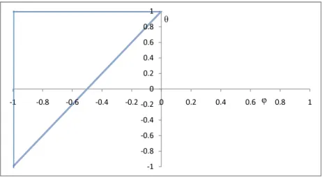
We numerically demonstrate the value of information sharing and the potential for a simple AR(1) demand to result in benefit of information sharing for an upstream player. In all figures in this section, we assume that the retailer observes ARMA(1,1) demand with leadtime `1 = 1. In
Figure 1, the enclosed region shows those values ofφandθ1of the retailer’s demand model such that
the enclosed region consists of one quarter of all possible ARMA(1,1) demand configurations for the retailer if the leadtime is 1. In Figure 2, we study the same situation as mentioned above except here we measure the value of information sharing for the supplier in terms ofln(V) whereV = M SF EM SF EN SS
and we assume that the retailer observes ARMA(1,1) demand with φ = −.7. As θ1 approaches
.3, the value of information sharing approaches infinity since β1 = 1 +φ−θ1 approaches 0 (See
Proposition 2). From Figure 1, it can be seen that even when the retailer observes AR(1) demand, i.e,. whenθ1 = 0, the supplier’s demand will not be invertible with respect to the retailer’s shocks
ifφ < −.5. Hence our paper is crucial to understanding how a simple AR(1) demand propagates
along a supply chain and the value of information sharing within it. For example, if φ=−.6 and
θ1= 0, if`1= 1, the retailer’s order to the supplier is given byD2,t=.6D2,t−1+d+²1,t−1.5²1,t−1. Hence{D2,t}is not invertible with respect to{²1,t}. In the event the retailer does not share with the
supplier and`2 = 1, then the supplier’s MSFE is.36σ21 whereas if the supplier would sub-optimally
use the GGS forecast, the MSFE would be.52σ2
1, i.e. M SF E
GGS M SF E = 139.
Proposition 2 If `k≤J˜k, then there exists unbounded gain to player kfrom player k−1 sharing its full information shocks.
Proof. Since `k ≤J˜k, it follows that if playerk−1 shares its full information shocks with player
k, then ωk,i = 0 for 0≤i≤`k−1 and hence the mean square forecast error of leadtime demand,
σ2
k
P`k−1
i=0 ωk,i2 , under information sharing is 0. On the other hand, if playerk−1 does not share with playerk, then by Theorem 1 (III) , Jk= 0,ωk,0 = 1 and henceM SF EkN S ≥σk2>0.
2
Remark 2 Proposition 2 demonstrates where there exists unbounded gain to playerk from player k−1sharing its full information shocks. However, as can be seen from Figure 2, there can be great value to information sharing even in a neighborhood around such a configuration where there exists unbounded value of information sharing.
full information shocks or shares nothing. There, we demonstrate that it is possible for playerk’s
demand not to be invertible with respect to playerk−1’s shocks and yet there is no value to player
k for player k−1 to share its demand. Besides being mathematically interesting, this also is in
contrast to results of GGS.
6
Shock Sharing versus Demand Sharing
In this section, we assume that the retailer through player k−2 shared either nothing or the
equivalent of their full information shocks. We show that under these assumptions the value to playerkof receiving demand information shared by playerk−1 may be different than the value to
player k of receiving shocks shared by player k−1. However, we leave the study of the structure
of the propagation of demand when sharing of demand information occurs as well as research on the related topic of sharing between non-contiguous players to future work.
Here, we discuss specific scenarios where {Dk,t} is not invertible with respect to{²k−1,t}under which there are various possible relationships among MDk−1
t , MDtk, MtDk−1,Dk, and M²tk−1. We show that the value to player k of receiving demand information shared by player k−1 may be :
nonexistent; positive, but less than that obtained from player k−1 sharing its shocks {²k−1,t}; or positive and equivalent to that obtained from playerk−1 sharing its shocks {²k−1,t}.
The first scenario we consider is where k= 2 and{D2,t}is not invertible with respect to{²1,t}.
Here, it is equivalent for the retailer to share its demand or its full information shocks with the supplier since{D1,t} is always invertible with respect to{²1,t} and henceMD2
t ⊂ MDt1 =M²t1. For the rest of this section, we consider the scenario where k= 3 and {D2,t} is not invertible
with respect to {²1,t} but the retailer shared the equivalent of its full information shocks with
the supplier (player 2). We further assume that {D3,t} is not invertible with respect to {²2,t}, ˜
shared its shocks with the supplier,²2,t =β1²1,t,
φ(B)D2,t = d+ ˜θ2(B)(β1²1,t)
φ(B)D3,t = d+ ˜θ3(B)(β1β2²1,t). (14)
Since{D2,t}is not invertible with respect to{²1,t}and ˜J2= 0, at least one root of ˜θ2(z) lies within
the unit circle, but not at 0. Similarly, at least one root of ˜θ3(z) lies within the unit circle, but not
at 0. From these facts along with (14),
²1,t = (φ(B)D2,t−d)˜θ
−1 2 (B)
β1
= (φ(B)D3,t−d)˜θ
−1 3 (B))
β1β2
. (15)
Multiplying both sides of (15) by ˜θ2(B)˜θ3(B)φ−1(B), we obtain
β2θ˜3(B)D2,t= ˜θ2(B)D3,t+ d
φ(1)
h
β2θ˜3(1)−θ˜2(1)
i
. (16)
It is possible that ˜θ3(z) and ˜θ2(z) have common roots. Denote ˜θm
3 (z) and ˜θ2m(z) as the polynomials
associated with (16) after the cancelation of common factors. After canceling common factors, it follows from (16) that
β2θ˜3m(B)D2,t = ˜θm2 (B)D3,t+φ(1)d
h
β2θ˜m3 (1)−θ˜m2 (1)
i
. (17)
Therefore, {D2,t} can be represented as a constant plus a linear combination of only present
and past values of{D3,t} if and only if ˜θm
3 (z) has all of its roots outside the unit circle. Similarly, {D3,t}can be represented as a constant plus a linear combination ofonly present and past values of
{D2,t}if and only if ˜θm2 (z) has all of its roots outside the unit circle. There are thus four potential
cases regarding the relationship amongMD2
t ,MDt3 andMDt2,D3. In each of the four cases below, if the supplier shared its shocks or nothing with player 3, then player 3 can determine its best linear forecast of leadtime demand as described in Section 5. We now focus on the potential benefit to player 3 of receiving demand shared by the supplier.