REGRESSION LEARNING FOR 2D/3D IMAGE REGISTRATION
Chen-Rui Chou
A dissertation submitted to the faculty of the University of North Carolina at Chapel Hill in partial fulfillment of the requirements for the degree of Doctor of Philosophy in
the Department of Computer Science.
Chapel Hill 2013
Approved by:
Stephen M. Pizer Sha X. Chang
David S. Lalush
c
2013
ABSTRACT
CHEN-RUI CHOU: REGRESSION LEARNING FOR 2D/3D IMAGE REGISTRATION.
(Under the direction of Stephen M. Pizer.)
Image registration is a common technique in medical image analysis. The goal of im-age registration is to discover the underlying geometric transformation of target objects or regions appearing in two images. This dissertation investigates image registration methods for lung Image-Guided Radiation Therapy (IGRT). The goal of lung IGRT is to lay the radiation beam on the ever-changing tumor centroid but avoid organs at risk under the patient’s continuous respiratory motion during the therapeutic procedure.
ACKNOWLEDGEMENTS
TABLE OF CONTENTS
1 Introduction 1
1.1 Image Registration for Medical Image Analysis . . . 1
1.2 Challenges of Image Registration as Guidance for Radiation Therapy . 2 1.3 A Brief Outline of the Proposed Methods . . . 3
1.3.1 Linear Regression Learning . . . 4
1.3.2 Non-linear Regression Learning . . . 4
1.3.3 Locally-linear Regression Learning . . . 4
1.4 Thesis and Contributions . . . 5
1.5 Overview of Chapters . . . 6
2 Image Registration 7 2.1 Parametric Registration . . . 8
2.1.1 Global Parameterization by Linear Analysis (PCA) . . . 9
2.1.2 Local Parameterization by B-Splines . . . 10
2.2 Non-parametric Registration . . . 11
3 Image-Guided Radiation Therapy 15 3.1 Treatment planning . . . 15
3.2 Treatment-time Image Guidance . . . 17
3.3 Treatment Imaging Geometry . . . 18
3.3.2 Nanotube Stationary Tomosynthesis (NST) . . . 19
3.4 Projection Intensity Pattern by a Local Normalization Scheme . . . 20
3.4.1 Local Gaussian Normalization . . . 20
3.4.2 Histogram Matching . . . 21
4 Transformation Parameterization for IGRTs 23 4.1 Rigid Transformation . . . 23
4.2 Non-Rigid Transformation . . . 23
4.2.1 Deformation Shape Space and Mean Image Generation . . . 24
4.2.2 Statistical Analysis . . . 25
5 Linear Regression Learning (CLARET) 26 5.1 General 2D/3D Registration . . . 26
5.2 Efficient Linear Approximation of ∆C . . . 29
5.3 Linear Regression Learning . . . 29
5.3.1 Learning Regressions from Residues to Shape Parameters . . . . 30
5.3.2 Efficient Sampling . . . 31
5.3.3 Linear Assumption for Iterative Estimation . . . 31
5.4 Experimental Setup . . . 32
5.4.1 Head-and-neck IGRT . . . 33
5.4.2 Lung IGRT . . . 33
5.5 Results . . . 36
5.5.1 Rigid Registration Results . . . 36
5.5.2 Non-rigid Registration Results . . . 40
6 Nonlinear Regression Learning 53 6.1 2D/3D Registration Framework . . . 54
6.2.1 Metric Learning and Kernel Width Selection . . . 55
6.2.2 Linear-Regression Implied Initial Metric . . . 57
6.2.3 Optimization Scheme . . . 58
6.3 Results . . . 58
6.3.1 Synthetic Tests . . . 59
6.3.2 Real Tests . . . 60
6.3.3 The Learned Metric Basis Vector . . . 62
7 Locally-linear Regression Learning 64 7.1 Method Overview . . . 65
7.2 Training Stage . . . 66
7.2.1 Deformation Space Formulation . . . 66
7.2.2 Training Space Sampling . . . 66
7.2.3 Training Space Partitioning . . . 67
7.2.4 Local Regression Learning . . . 68
7.2.5 Decision Forest Training . . . 68
7.3 Treatment Application Stage . . . 69
7.3.1 Forest Classification . . . 70
7.3.2 Regression Estimation . . . 70
7.4 Results . . . 70
7.4.1 The Datasets . . . 71
7.4.2 Synthetic Tests . . . 72
7.4.3 Real Tests . . . 77
8 Comparisons 80 8.1 Synthetic Tests . . . 80
8.1.2 Global vs. Local CLARET (noniterative) . . . 83
8.1.3 REALMS vs. Others . . . 83
8.2 Real Tests . . . 84
8.3 Which One is the Winning Method? . . . 85
Chapter 1: Introduction
1.1 Image Registration for Medical Image Analysis
Image registration is a common technique in medical image analysis. The goal of image registration is to discover the underlying geometric transformation of target objects or regions appearing in two images. In many medical situations doctors need to understand transformation of the target (e.g., organs or tissues) between two images before making any medical decisions. Therefore, image registration is a fundamental task of medical image analysis.
Many current medical imaging techniques compute 3D image data by reconstruc-tion of a collecreconstruc-tion of 2D projecreconstruc-tion images acquired at various angles, e.g., CT (Com-puted Tomography). Their 3D image quality (volumetric information) increases with the number of angular samples of projection images. Image registration between two high-quality 3D images has shown good estimation of the underlying transformation (Vercauterenet al.(2009); Rohret al.(2001); Christensenet al.(1996a); Rueckertet al. (1999); Pluimet al. (2003)).
1.2 Challenges of Image Registration as Guidance for Radiation Therapy
One medical application of registration is lung Image-Guided Radiation Therapy (IGRT). The goal of lung IGRT is to lay the radiation beam on the ever-changing tumor centroid under the patient’s continuous respiratory motion but to avoid organs at risk (OAR) during the therapeutic procedure. Therefore, image registration between high-quality 3D images can not provide timely information of the tumor location.
Recent advances of IGRT registration methods suggest a new direction: 2D/3D image registration. 2D/3D image registration for IGRT estimates the underlying 3D transformation between a high-quality 3D image acquired at planning time and a small set of projections that can be quickly acquired at treatment time.
2D/3D image registration computes 3D transformations based on information of the 2D projection intensities. It estimates a 3D transformation where the projection intensities of the transformed 3D volume match the target projection intensities. Due to the mismatch in the registration dimensions, the 2D/3D image registration problem is ill-posed: the unknowns (transformations at all 3D pixels) are orders of magnitude more than the given constraints (intensity differences at all projection pixels). Therefore, in order to solve the 2D/3D image registration, one needs to impose more spatial or temporal constraints on the transformation.
At treatment time, with the constrained and parameterized transformations the 2D/3D image registration method now is a more well-posed problem with a low-dimensional unknown space of parameters: optimizing the transformation parameters (dimension<10) by matching the target projection intensities (dimension>100,000) and the projection intensities of the estimated 3D volume.
Another challenge for registrations in IGRT is the computation time. To have a real-time1 registration method that can deal with more than 10 registrations per second, the optimization-based 2D/3D image registration approach (Li et al. (2011a, 2010)) above requires GPU acceleration on the iterative calculation of the objective function’s Jacobian and a good initialization of the parameters (Ch. 2). Given the fact that a good initialization of the optimizing parameters is not normally available, in this dissertation I seek a new solution by regression learning that can provide efficient 2D/3D image registration in IGRT without requirements on initialization.
1.3 A Brief Outline of the Proposed Methods
The idea of regression learning is as follows: if we have a way to sample the patient’s credible 3D transformations and simulate the corresponding projection intensity pat-terns, at treatment-planning time we can create a patient-specific training set of projec-tion intensity and transformaprojec-tion pairs and thereby learn a set of regression funcprojec-tions that map projection intensities to 3D transformations. Using this at treatment time, given a projection intensity pattern we can apply those learned regression functions and efficiently estimate the patient’s deformation.
In this dissertation, three types of regression functions (linear, nonlinear, and locally-linear regressions) have been investigated for learning from the patient-specific training
110 registrations per second is considered as real-time computation given the fact that current CBCT
sets.
1.3.1 Linear Regression Learning
The linear-regression-learning method is called Correction via Limited-Angle Residues in External beam Therapy (CLARET), which learns a global linear regression function that maps projection intensities into the transformation parameters. At treatment time the patient’s transformation parameters can be estimated iteratively (CLARET-itr) or non-iteratively (CLARET-non(CLARET-itr) by the projection residues between the target projection and the calculated projection of currently-estimated image (Ch. 5). The purpose of iterating the estimation is to have a more accurate registration. The method has appeared in Chou et al. (2010b,a, 2011b,c,a, 2013).
1.3.2 Non-linear Regression Learning
The nonlinear-regression-learning method is called Registration Efficiency and Accu-racy through Learning Metrics on Shape (REALMS). To relax the strong linear assump-tion (between transformaassump-tion parameters and projecassump-tion intensities) made in CLARET, REALMS learns distance metrics for non-linear kernel regressions between the trans-formation parameters and the projection intensities. This method is a non-iterative method: at treatment time, the transformation parameters are interpolated once from the training parameters weighted by kernels equipped with the learned distance metric (Ch. 6). The method has been appeared in Chouet al. (2012); Chou and Pizer (2012).
1.3.3 Locally-linear Regression Learning
The local-learning version of the non-iterative CLARET is called Local-CLARET (L-CLARET). The goal of L-CLARET is to find a balance between the strong linear assumption in CLARET and the time-consuming non-linear learning in REALMS. In-stead of learning a global linear mapping, L-CLARET learns linear regression mappings for every local training parameter neighborhood to obtain better regression fitting. At treatment time, the acquired projection is first classified into a training local neighbor-hood by efficient decision forest classification based on projection image visual features. Second, the transformation parameters are estimated with the linear regression of this local training neighborhood (Ch. 7). The method has appeared in Chou and Pizer (2013).
1.4 Thesis and Contributions
Thesis: Regression learning provides a new solution to the image registration problem. Learning patient-specific intensity-to-shape regressions allows efficient, accurate, and robust 2D/3D image registration for image-guided radiation therapy.
The contributions of this dissertation are the following:
(1) The development of four regression-learning-based 2D/3D image registration meth-ods for image-guided radiation therapy.
a. CLARET (Correction via Limited-Angle Residues in External Beam Therapy) b. REALMS (Registration Efficiency and Accuracy through Learning Metric on
Shape)
c. L-CLARET (Local CLARET)
(3) The iterative versions of the four methods in(1): enhancing registration accuracy by iterative estimation.
(4) The development of scattering removal and intensity correction on the digitally reconstructed radiographs (DRR) and the treatment-time radiographs to allow the commensurate intensity comparison required by the proposed methods.
(5) The evaluation of CLARET, L-CLARET and REALMS for lung IGRT with sim-ulated and real patient cone-beam radiographs, including comparisons to an optimization-based 2D/3D registration approach.
(6) The evaluation of CLARET for head-and-neck IGRT with simulated and real patient Nanotube Stationary Tomosynthesis (NST) (Maltz et al. (2009)) radio-graphs.
1.5 Overview of Chapters
Chapter 2: Image Registration
Image registration, i.e., finding the underlying geometric transformation between two images, is widely used in many fields. That is, given a source imageI0 : Ω⊂Rd→R
(d is the image dimensionality, e.g., d = 2,3) and a target image I1 : Ω → R, find
a reasonable transformation map φ : Ω → Rd such that the transformed source
im-age I0(φ) is similar to the target image I1 (Modersitzki (2004)). In computer vision,
for example, scientists use image registration to understand pixel correspondence in stereographic projections for 3D scene reconstruction (Blais and Levine (1995)). In medical image analysis, scientists use image registration to understand possible trans-formations appearing in a sequence of images for pathological staging of a disease (Fox et al.(2001)), population analysis (Lorenzenet al. (2006); Cooteset al. (2004); Bhatia et al.(2004); Davatzikoset al.(1996)), atlas based segmentations (Isgum et al.(2009); Aljabar et al. (2009); Collins and Evans (1997); Wu et al. (2007)), or aligning images from multiple modalities of the same patient (D’Agostino et al. (2003); Gaens et al. (1998); Roche et al. (1998); Maeset al. (1997)). With its popularity, there is a variety of image registration methods developed for various purposes. The classic variational approach for image registration can be formulated as an energy minimization process that finds a displacement fieldu: Ω→Rd between two images through minimizing an
energy function consisting of a data attachment termED and a regularization termER
u=arg
u min ED(I0(φ), I1) +λER(u), (2.0.1)
whereφ=Id+u; λis the Lagrange multiplier (Bellman (1986)). The data attachment term measures the image dissimilarity using some distance measure on intensities:
L2-norm (Belongieet al.(2002); Rueckertet al.(1999)), cross-correlation (Lewis (1995);
Rocheet al.(1998)), mutual information (Pluimet al.(2003); Maeset al.(1997); Gaens et al.(1998); D’Agostino et al. (2003)). The regularization term uses a physical model that regularizes either the output displacement field: elastic model (Rohret al. (2001)) and diffusion model (Horn and Schunck (1981)) or the time-varying velocity field: fluid model (Christensen et al. (1996a)). With this framework, image registration can be classified into two types: methods using a parameterized transformation (2.1) and methods using non-parameterized transformation (2.2).
2.1 Parametric Registration
Image registration without regularization, i.e., led solely by the data attachment en-ergy ED in Eq. 2.0.1, is ill-posed: the dimension of the unknown displacements is
Component Analysis (PCA): Li et al. (2011a); Liu et al. (2010); Chou et al. (2013), trigonometric functions: Reddy and Chatterji (1996); Chen et al. (1994), Radial Ba-sis Functions (RBF): Chui and Rangarajan (2003); Fornefett et al. (2001); Bookstein (1989)). In the following sections, I respectively describe the global parameterization by PCA (Section 2.1.1) and the local parameterization by B-Splines (Section 2.1.2).
2.1.1 Global Parameterization by Linear Analysis (PCA)
If there exists a set of displacement fields of the target object/region, one can parame-terize the transformation globally by doing linear analysis based on this a prior displace-ment fields, e.g., PCA. This global parametric method assumes that the displacedisplace-ment fieldu at pixel/voxel locationxcan be represented by m parametersc= (c1, c2, ..., cm)
as the scores on their eigenmode basis functions b={b1, b2, ..., bm}:
u(x,c,b) =
m
X
k=1
ckbk(x), (2.1.1)
whereck ∈Rand bk : Ω→Rd.
With this parameterization, we can re-write the optimization in Eq. 2.0.1 as follows:
c=arg
c=arg c
min ˆ
Ω
(I0(x+u(x,c,b))−I1(x))2dx (2.1.3)
The final displacement field can be computed by Eq. 2.1.1, using the basis functions b and the optimized parameters c.
The advantage of this parametric method is that the space of transformations can be greatly reduced by PCA (Liet al.(2011b); Liuet al.(2010); Liet al.(2011a)), so the registration optimization problem is well-posed (#unknown transformation parameters
#known intensity pairs). With only a few parameters to optimize, the method is
also efficient.
The downside of this parametric approach is that it cannot produce a displacement field outside of the space spanned by those eigenmode basis functions. This constraint discourages registration of objects of high shape variability where no prior displacement sets can include all its variations.
2.1.2 Local Parameterization by B-Splines
If there is no a priori knowledge of the object’s transformation, one can still parame-terize the transformation space by B-Splines (De Booret al.(1978)) and optimize over the B-Spline parameters for registration. For example, Free-Form Deformation (FFD) registration (Rueckert et al. (1999, 2006)) uses cubic B-Spline functions to deform an object by manipulating an underlying mesh of control points. The resulting deforma-tion produces a smooth and continuous transformadeforma-tion. FFD registradeforma-tion samples an
nx ×ny ×nz mesh of control points c = {c1,1,1, ..., ci,j,k, ..., cnx,ny,nZ} at grid points
(d= 3) and takes transformations at control pointsφ ={φ1,1,1, ..., φi,j,k, ..., φnx,ny,nZ}
(whereφ : Ω→Rd) as the parameters. FFD registration minimizes the image
at voxels (x, y, z) other than the control points are interpolated by the four cubic B-Spline functionsb={b0, b1, b2, b3}(wherebk : Ω→R) among the nearby 3×3×3 = 27
control points.
φ(x, y, z) =
3 X p=0 3 X q=0 3 X r=0 bp(
x nx − x nx )bq(
y ny − y ny )br(
z nz − z nz
)φi+p, j+q, k+r, (2.1.4)
wherei=jnx
x
k
−1, j =jny
y
k
−1, k =jnz
z
k
−1,b0(∆) = (1−∆)3
6 , b1(∆) =
(3∆3−6∆2+4)
6 ,
b2(∆) =
(−3∆3+3∆2+3∆+1)
6 , and b3(∆) = ∆3
6 .
The advantages of B-Spline-based FFD registration are (1) it can parameterize the transformation without a priori information, (2) B-Splines are locally controlled, which makes it computationally efficient (that is, it doesn’t need to update the whole image volume for a parameter update), and (3) it can optimize over various transformation scales by multi-level registrations using sparse-to-dense control points (Rueckert et al. (1999, 2006)). The registration solution is also unique when the number of control points is less than one third of the number of image voxels.
2.2 Non-parametric Registration
In FFD registration, when sampling control points at every image voxel, the resulting transformation will have the most flexibility. Like FFD registration that uses fully-sampled control points, non-parametric registration grants an independent transfor-mation for each voxel. However, this high flexibility makes the registration problem ill-posed. To make it more well-posed, scientists have come up with various regular-ization approaches that impose physical models to the transformations. Based on the regularization types, they can be briefly categorized into the following registrations.
and Modersitzki (2002)) penalize gradient magnitudes of the displacement field in the regularization energy:
ERdif f(u) = 1 2 n X d=1 ˆ Ω
k∇ud(x)k2dx (2.2.1)
Elastic registrations (Rohr et al. (2001); Broit (1981); Bajcsy and Kovacic (1989); Christensen et al. (1994a,b); Gee et al. (1997)) penalize the elastic potential of the displacement field u in the regularization energy:
ERelas(u) = ˆ
Ω λ+µ
2 k∇ ·u(x)k
2 + µ 2 n X d=1
k∇ud(x)k
2
dx (2.2.2)
where the constantsλ,u >0 describe material properties.
However, both of the above regularization energies discourage transformations of large displacements. The recently popular Large Deformation Diffeomorphic Metric Mapping (LDDMM) framework using the fluid-flow analogy (Christensenet al.(1996a); D’Agostino et al. (2003); Bro-Nielsen and Cotin (1996); Christensen et al. (1996b); Christensen (1994); Dupuis et al. (1998)) allows large displacements. Instead of regu-larizing the displacement fields, it regularizes the time-dependent velocity fields from fluid mechanics:
ERf luid(u) = ˆ
Ω
ˆ 1
t=0
kvt(x)kV dx, (2.2.3)
where the flows vt: Ω → V (t ∈ [0,1]) are time-dependent velocity fields that are
elements of a Hilbert spaceV: Ω→Rd with inner product <·,·>
V. The norm kvtkV
can be expressed as< Lvt, Lvt>L2 regularized by the differential operatorLfrequently
taken from fluid mechanics: L=α∇2+β(∇·)∇+γandα, β, γ >0. Theαterm controls
The fluid-flow-based LDDMM framework can be written in the following form (Beg et al. (2005)):
v = arg min
v : ˙φt=vt(φt)
ˆ
Ω
ˆ 1
t=0
kvt(x)kV dt+
1
σ2
I0(φ−1t=1(x))−I1(x)
L2dx (2.2.4)
where φt=1(x) describes the final transformation (t= 1) at the voxel location xin the
“target” imageI1. The transformation at timeTof a voxel locationxcan be integrated
as follows:
φT(x) = φt=0(x) +
ˆ T
0
vt(φt(x))dt (2.2.5)
whereφt=0(x) =x.
“As shown in Dupuiset al. (1998) and Trouve (1995), enforcing a sufficient amount of smoothness on the elements of the spaceV of allowable velocity vector fields ensures that the solution to the differential equation ˙φt = vt(φt), t ∈ [0,1], vt ∈ V is in the
space of diffeomorphisms.”1 Therefore, the solution satisfying Eq. 2.2.4 is an LDDMM solution in the following two senses: (1) as shown in Christensen et al. (1996b) the fluid-flow approach provides a large deformation coordinate system transformation, and (2) as shown in Miller and Younes (2001), Trouve (1995) and Miller et al. (2002), in contrast to Christensenet al.(1996b), the length of the shortest path inf´t1=0kvt(x)kV dt
connecting imagesI0 toI1 defines a metric in the image space.
However, LDDMM is not the only method that produces diffeomorphic transfor-mations. Many other registration methods (Vercauteren et al. (2009); Rueckert et al.
(2006); Ashburner (2007)) have been recently revised to guarantee large and diffeomor-phic transformations by regularizing the time-dependent velocity fields.
Chapter 3: Image-Guided Radiation Therapy
3.1 Treatment planning1
A CT image taken of patients in the treatment position is used for the radiotherapy treatment planning process. Using this image, the tumor and the normal organ struc-tures at risk are segmented, the radiation field is designed, and the radiation dose is computed. This reference CT should contain information as to where volumetrically the tissue to be treated is. There are three main volumes in radiotherapy planning. The first is the position and the extent of gross tumor, i.e., what can be seen or im-aged; this is known as the gross tumor volume (GTV). Developments in imaging have contributed to the definition of the GTV. The second volume contains the GTV, plus a margin for sub-clinical disease spread which therefore cannot be fully imaged; this is known as the clinical target volume (CTV). The CTV is important because this volume must be adequately treated to achieve cure. The third volume, the planning target volume (PTV), allows for uncertainties in planning or treatment delivery. It is a geometric concept designed to ensure that the radiotherapy dose is actually delivered to the CTV. See Fig. 3.1.1 for visualization of those target volumes. Radiotherapy planning must also consider critical normal tissue structures, known as organs at risk (OAR). In some specific circumstances, it is necessary to add a margin analogous to the PTV margin around an OAR to ensure that the organ cannot receive a higher-than-safe
dose; this gives a planning organ at risk volume. This applies to an organ such as the spinal cord, where damage to a small amount of normal tissue would produce a severe clinical manifestation (Burnetet al. (2004)).
Figure 3.1.1: Planning volumes for a patient with a WHO grade 4 glioma (glioblas-toma). (a) Planning CT showing a contrast-enhancing tumor. (b) The GTV is the visible tumor. (c) A margin for microscopic spread has been added to make the CTV; the margin is the same in all directions except that it is restricted by the skull. (d) The PTV has added to the CTV to account for uncertainties in planning and execution of treatment; this extends beyond the inner table of the skull. (Burnet et al. (2004))
Figure 3.1.2: Treatment planning through simulation of the radiation. The outermost pink contour is the PTV. (Vandemeulebroucke et al. (2009))
3.2 Treatment-time Image Guidance
Fig. 3.2.1 shows a typical IGRT environment: an adjustable patient couch and a rotating Cone-Beam CT imager (CBCT, 3.3.1) mounted on a linear accelerator. Before radiation treatment, a 3D image acquired by the CBCT imager will be used to measure the patient’s setup deviation between the planning and treatment CT volumes. The amount of setup deviation can be calculated by 3D/3D image registration of the volume of interest to allow accurate setup for daily treatment. The setup deviation can then be corrected rigidly by shifting and rotating the couch position and orientation such that the CT volumes match.
real-time.
Figure 3.2.1: An Elekta radiation treatment machine (Capital Radiation Therapy (2013)) with an x-ray imager mounted.
The clinical goal for registration accuracy is 2 mm in the patient plane. The de-tected patient transformations at treatment deliveries can be used for a follow-up dose accumulation study. The purpose of the dose accumulation study is to allow the next treatment fraction to compensate for those regions that have been over-dosed and those regions that have been under-dosed.
3.3 Treatment Imaging Geometry
3.3.1 Cone-beam CT (CBCT)
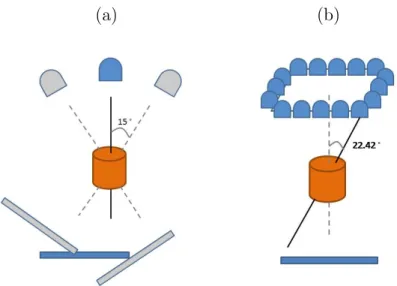
A CBCT is a rotational imaging system with a single radiation source and a planar detector, which may be mounted on a medical linear accelerator. This pair rotates by an angle of up to 2π during IGRT, taking projection images Ψ during traversal (Fig. 3.3.1(a)). A limited-angle rotation provides a shortened imaging time and lowered imaging dose. For example, a 5◦ rotation takes ∼1 second. In my application, CBCT projections were acquired in a half-fan mode. Half-fan mode means that the imaging panel (40 cm width by 30 cm height, source-to-panel distance 150 cm) is laterally offset 16 cm to increase the CBCT reconstruction diameter to 46 cm. The method’s linear operators are trained for projection angles over 360 degrees at 1 degree intervals beforehand at planning time. At treatment time my proposed methods will choose a learned regression that is closest to the current projection angle.
3.3.2 Nanotube Stationary Tomosynthesis (NST)
(a) (b)
Figure 3.3.1: (a) Short arc CBCT geometry: rotational imaging system depicting a 30◦arc. The image detector is laterally offset for half-fan acquisition. (b) The NST geometry: stationary sources array with angle θ = 22.42◦
3.4 Projection Intensity Pattern by a Local Normalization Scheme
X-ray scatter is a significant contributor to the cone-beam CT projections. However, the regression estimators of my proposed methods are not invariant to the projection intensity variations caused by x-ray scatter. Therefore, I implemented a normalization filter (3.4.1) and a subsequent histogram matching scheme (3.4.2) that when applied to both learning-time computed projections and registration-time target projections, generate commensurate intensities between these two images.
3.4.1 Local Gaussian Normalization
meanµ0(x1, x2) from the raw pixel value Ψ(x1, x2) and divide it by a Gaussian-weighted
standard deviation σ0(x1, x2).
Ψ0(x1, x2) =
Ψ(x1, x2)−µ0(x1, x2) σ0(x
1, x2)
(3.4.1)
µ0(x1, x2) =
Px1+A ξ=x1−A
Px2+B
η=x2−B[K(ξ, η; 0, w)·Ψ(ξ, η)]
Px1+A ξ=x1−A
Px2+B
η=x2−BK(ξ, η; 0, w)
(3.4.2)
σ0(x1, x2) =
Px1+A ξ=x1−A
Px2+B
η=x2−B[K(ξ, η; 0, w)·Ψ(ξ, η)−µ 0(x
1, x2)]2
Px1+A ξ=x1−A
Px2+B
η=x2−BK(ξ, η; 0, w)
!12
(3.4.3)
where 2A+ 1 and 2B + 1, respectively, are the number of columns and rows in the averaging window centered at (x1, x2); the function K is an isotropic Gaussian with
marginal standard deviation w. I choose A, B, and w to be appropriate values (dis-cussed in Ch. 5.5.2) to perform a local Gaussian-weighted normalization for my target problem.
3.4.2 Histogram Matching
In order to correct the intensity spectrum differences between the normalized learning projection Ψ0learning and the normalized target projection Ψ0target, a function Fω of
in-tensity to achieve non-linear cumulative histogram matching within a region of interest
ω is applied. To avoid having background pixels in the histogram, the region ω is de-termined as that pixel set whose intensity values are larger than the mean value in the projection. That is,Fω is defined by
where Hf is the cumulative histogram profiling function. The histogram matched
intensities Ψ?target (Fig. 3.4.1(c)) are calculated through the mapping:
Ψ?target = Ψ0target◦Fω (3.4.5)
(a) (b)
(c) (d)
Chapter 4: Transformation Parameterization for IGRTs
To make the 2D/3D image registration robust, my methods limit the patient’s trans-formation to a shape space. In order to have efficient registration, my methods also represent the patient’s transformation with low-dimensional global parametersC. The following sections (4.1 and 4.2) detail the shape space formulation and parameterization for both rigid and non-rigid transformations.
4.1 Rigid Transformation
In IGRT sites where the patient’s motion is mainly rigid (e.g., head and neck), the patient’s motion can be modeled explicitly as the variation in the Euler’s six dimensional rigid space:
C= (tx, ty, tz, rx, ry, rz) (4.1.1)
wheretx,ty,tz are the translation amounts in cm along the world’s coordinate axesx,
y, z, respectively; and rx, ry, rz are the rotations in degrees about the image center,
around the world coordinate axes x,y, and z, in succession.
4.2 Non-Rigid Transformation
calculated through principal component analysis (PCA). In lung and abdominal IGRT where the patient’s deformation is dominated by respiration, a cyclically varying set of 3D images across respiration cycle{Jτ: Ω⊂R3 over timeτ}are available at treatment
planning time. From these a mean image ¯J and a set of deformations φτ: Ω → R3
between Jτ and ¯J can be computed. The basis deformations are chosen to be the
primary eigenmodes of the set of deformations{φτ}. The computed mean image ¯J will
be used as the reference image I throughout this dissertation. The following sections will detail the computation pipeline.
4.2.1 Deformation Shape Space and Mean Image Generation
In order to obtain a reference image that better represents the mean point in the patient’s respiratory cycle, my methods compute a Fr´echet mean image J that is an intrinsic mean image on the patient’s respiratory manifold. The Fr´echet mean imageJ
can be computed by anLDDMM (Large Deformation Diffeomorphic Metric Mapping) framework (Beg et al. (2005)) from the cyclically varying set of 3D images {Jτ over
timeτ}. The Fr´echet mean, as well as the diffeomorphic deformationsφfrom the mean to each imageJτ, are computed using a fluid-flow distance metricdf luid(Lorenzenet al.
(2006)):
J = arg
J
min
N
X
τ=1
df luid(J, Jτ)2 (4.2.1)
=arg J min N X τ=1 ˆ 1 0 ˆ Ω
||vτ,γ(x)||2dxdγ+
1
α2
ˆ
Ω
||J(φ−1τ (x))−Jτ(x)||2dx
!
(4.2.2)
where Jτ(x) is the intensity of the pixel at position x in the image Jτ, vτ,γ is the
fluid-flow velocity field for the image Jτ in flow time γ ,α is the weighting variable on
φτ(x) =x+
´1
0 vτ,γ(x)dγ.
The mean image J and the deformations φτ are calculated by gradient descent
optimization. The set{φτ overτ}can be used to generate the deformation shape space
by the following statistical analysis.
4.2.2 Statistical Analysis
Starting with the diffeomorphic deformation set{φτ}, one can represent this
diffeomor-phic set by doing analysis on their initial momenta (Wanget al.(2007); Zhong and Qiu (2010); Niethammer et al. (2011)), e.g., on vτ,0 for registering Jτ to ¯J. However, the
goal of the IGRT application is to do fast, and probably real-time, image registration. Although registration leveraging the analyzed space of the initial momenta will help to generate realistic diffeomorphic transformations constrained to the transformation space a priori, the registration evolution at treatment time is still time-consuming. Therefore, instead of analyzing the space of the initial momenta, my methods find a set of linear deformation basis functions φipc by doing PCA on the diffeomorphic set. The linear combination of the scoresλiτ (basis function weights) and the corresponding basis functions φipc yield a final transformation φτ in terms of these basis functions.
φτ =φ+ N
X
i=1
λiτ ·φipc (4.2.3)
A subset of n eigenmodes that capture 95% of the total variation are chosen, and they let then basis function weightsλi form the n-dimensional parameterization C.
C = (c1, c2,· · · , cn) (4.2.4)
Chapter 5: Linear Regression Learning (CLARET)
This chapter begins with describing the general framework for the proposed 2D/3D registration methods (5.1). Section 5.2 details the proposed CLARET method that can do efficient registration using linear regression. The method’s application for rigid registration involves a multi-scale learning scheme that is also detailed in Section 5.3. I describe the experimental setup in Section 5.4. In Section 5.5 I show CLARET’s rigid (5.5.1) and non-rigid (5.5.2) 2D/3D registration results on synthetic and real test cases.
5.1 General 2D/3D Registration
The goal of the 2D/3D registration is to infer 3D transformations from 2D projections. I denote the projection intensity at pixel location x = (x1, x2) and projection angle θ
as Ψ(x;θ). Ψ(θ)⊂ R1×P (P is the dimension of the 2D projection). The registration
is formulated as an iterative process. LetI denote the 3D reference image andI(t) de-note the 3D image at iterationt. The estimated 3D image region’s motion/deformation parameters C(ˆ t): R → Rn (n is the number of parameters) define a geometric
trans-formationT(C(ˆ t)): Rn→
R3 in a space determined from one or more 3D images. I(t)
isT(C(ˆ t)) applied toI(0): Eq. 5.1.1.
I(t) = I(0)◦T(C(ˆ t))
I(0) = I
T(0) = Id
Idis the identity transformation.
The C(ˆ t) are calculated by the estimated parameter updates ∆C(ˆ t): R→Rn: Eq.
5.1.2.
ˆ
C(0) = 0
ˆ
C(t) = C(ˆ t−1) + ∆ ˆC(t)
(5.1.2)
The estimated parameter updates are obtained from the projection intensity residues R⊂R1×P (P is the dimension of the 2D projection) between the target 2D projections
Ψ(x;θ) and the computed projections P(x, I(t−1);θ)⊂R1×P of the transformed 3D
source image at iteration t−1: Eq. 5.1.3.
R[Ψ(x;θ),P(x, I(t−1);θ)] = Ψ(x;θ)−P(x, I(t−1);θ) (5.1.3)
After parameter estimation in each iteration, an image transformation (Eq. 5.1.1) is required in order to produce updated computed projections for the parameter esti-mation in the next iteration.
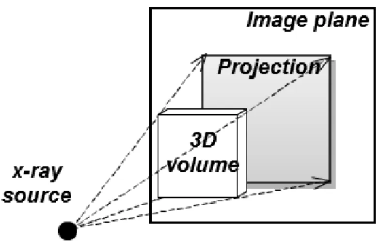
Figure 5.1.1: An x-ray projection is simulated by ray-casting on a 3D image volume. The dashed lines and arrows indicate the ray directions.
One way to obtain the estimated parameter updates ∆C(ˆ t) is by minimizing the sum of squared joint intensity residuesR†at various angles: θ1, θ2, ..., θAover the parameter
updates ∆C.
∆C(ˆ t) = arg ∆C
min
R
†
[Ψ,P(I(0)◦T(C(ˆ t−1) + ∆C))]
2
L2
(5.1.4)
The joint intensity residues R† ⊂ R1×P·A are defined as a concatenation over the
residues at available projection angles: R†= (Rθ1,Rθ2,· · · ,RθA) with
5.2 Efficient Linear Approximation of ∆C
Instead of adapting the traditional approach (Markeljet al. (2012); Zolleiet al. (2001); Li et al. (2010, 2011a); Russakoff et al. (2005, 2003); Weese et al. (1997); Fu and Kuduvalli (2008); Yao and Taylor (2003); Pickering et al. (2009); Sarrut and Clippe (2001); Rohlfing et al. (2002); Knaan and Joskowicz (2003)) as characterized in Eq. 5.1.4, I propose an alternative method (CLARET) to calculate the parameter updates ∆C⊂R1×n using a learned linear operatorW ⊂
RP·A×napplied to projection
intensi-ties. At each iteration of the registration, the method estimates the motion/deformation parameter updates by applying a linear operator to the current joint intensity residue R†⊂R1×P·A. That is,
∆C(ˆ t) =R†[Ψ,P(I(t−1))]·W, (5.2.1)
wheret = 1,2,· · · , tmax. Typically,tmax ≤10 are satisfactory.
The computation in Eq. 5.2.1 only involves matrix multiplications byW, computa-tion of the projeccomputa-tionsP, and subtractions (Eq. 5.1.3). Therefore, this registration can be computed efficiently. The calculation of the linear operator W involves a machine learning process described in detail in Section 5.3. Due to the machine learning process and the fast linear operation, the proposed CLARET method shows a more robust and faster registration than the optimization-based approach. See Section 5.5.2 for some comparisons.
5.3 Linear Regression Learning
operators in Section 5.3.1 and an efficient sampling strategy in Section 5.3.2.
5.3.1 Learning Regressions from Residues to Shape Parameters
The regression learning is similar to that in the Active Appearance Model (AAM) (Cootes et al. (2001)). As detailed in Chapter 4, a collection of shape parameters
{Cκ ⊂R1×n over cases κ} are sampled for learning. Each case is formed by a selection
of parameter settings. The training uses deviations from the reference image, such that ∆C = Cκ. Linear regression is used to correlate the sampled parameters Cκ in
theκth case with the co-varying projection intensity residue set{Rκ,θ ⊂R1×P over the
projection angles θ}. Rκ,θ(x) is computed as the intensity difference at pixel location
x= (x1, x2) between the projection at angleθof the mean imageI: Ω⊂R3 →R(or an
untransformed 3D image for the rigid case) and the projection of the imageI◦T(Cκ)
transformed with the sampled model parameter Cκ:
Rκ,θ(x) =P(x, I◦T(Cκ);θ)−P(x, I;θ) (5.3.1)
The method concatenates the residues at each projection angle to formulate a residue set in a vector R†κ ⊂R1×P·A = (R
κ,θ1,Rκ,θ2,· · · ,Rκ,θA) and computes a linear regression for all cases κ= 1,2,· · · , K:
C1 C2 .. . CK ≈
R†1 R†2 .. . R†K
The regression matrix W ⊂ RP·A×n that yield the best least square fitting to the
training set can be computed via a pseudo-inverse (Peters and Wilkinson (1970)):
W= (R†|R†)−1R†|C (5.3.3)
whereR ⊂RK×P·A and C⊂
RK×n.
5.3.2 Efficient Sampling
To provide adequate regression learning, C must be sufficiently sampled to capture all the shape variations. I have designed an efficient scheme to sample the shape parameters. Each shape parameterci is collected from the combinations of±3σi and 0
whereσi is the standard deviation of the basis function weightsλiobserved at treatment planning time.
5.3.3 Linear Assumption for Iterative Estimation
The linear assumption between deformation parameters and intensity residues allows the method to estimate parameter differences not only from a fixed reference deforma-tion but also from other deformadeforma-tions in the shape space. For example, assume there is a linear regression estimatorW that has been trained to estimate deformation param-eters C ⊂ RK×n from a collection of K training deformation parameter values. Now
consider two training parameter values Cp ⊂ R1×n and Cq ⊂ R1×n. Recall that the
linear regression estimatorW⊂RP·A×nis designed to estimate their values from their
intensity residues,R†p ⊂R1×P·AandR†
q ⊂R
1×P·Arespectively, from the reference DRR
(Eq. 5.3.4 and Eq. 5.3.5). R†p =P(I◦T(Cp))−P(I), andR†q =P(I◦T(Cq))−P(I).
Cq=R†q·W (5.3.5)
Notably, the regression result that estimates deformations from the mean to the training images can estimate the update in Cq to produce Cp from their intensity
residue difference: R†p−R†q as well. See Eq. 5.3.6.
Cp−Cq ={R†p−R
†
q} ·W (5.3.6)
With this property the method can perform efficient regression learning. It only needs to train deformation differences from a single reference deformation (C= 0), but the learned regression can estimate deformation update from any deformations as well. If the underlying deformation-to-intensity-residues relationship is not nearly linear, the error will propagate. Other proposed methods described in Ch. 6 and Ch. 7 are trying to relax this strong assumption of linearity.
5.4 Experimental Setup
5.4.1 Head-and-neck IGRT
In head-and-neck IGRT, the geometric differences of the skull between planning time and treatment time can be represented by a rigid transformation. Therefore, at treat-ment planning time, CLARET samples clinically feasible variations (±2 cm in transla-tions,±5◦ in rotations) in the Euler 6-space Cto capture the treatment-time patient’s motions. With a single planning CT I of the patient, the computed learning projec-tions P(I ◦T(C);θ) are generated by transformation of the feasible variations T(C) and projection from a given angle θ of the transformed 3D volume I◦T(C).
In the registration, CLARET iteratively applies the linear operators to estimate the rigid transformation from the 2D intensity residues formed by the difference between the normalized target projections Ψ? and the normalized projections computed from
the currently estimated rigid transformation applied to the planning-time 3D image.
5.4.2 Lung IGRT
A consideration in lung IGRT is that respiratory motion introduces non-rigid trans-formations. At treatment planning time, 10-phase RCCT set (Respiratory-Correlated CTs) collected at planning time serve as the cyclically varying 3D images {Jτ over the
phase τ}. This image set is used to generate the deformation shape space C. From these RCCTs, a Fr´echet mean image J and its deformations φτ to the corresponding
images Jτ are calculated via an LDDMM framework 4.2.2. Fig. 5.4.1(c) shows an
(a) (b) (c)
Figure 5.4.1: Coronal slices of (a) Respiratory-Correlated CT (RCCT) at the End-Expiration (EE) phase (b) RCCT at the End-Inspiration (EI) phase and (c) Fr´echet mean CT generated via the Large Deformation Diffeomorphic Metric Mapping frame-work from the RCCT dataset.
The deformation basis functionsφpcare then generated by PCA on the deformation
set{φτ over phaseτ}. Liuet al.(2010); Chouet al.(2013) has shown that a shape space
with three eigenmodes adequately captures 95% of the total variance of respiratory variations experienced at treatment time. Fig. 5.4.2 shows the first two principal deformation basis functions.
To generate feasible variations in the deformation space C for learning the linear operator W, CLARET samples parameters within three standard deviations of the means of the basis function weights derived from the RCCT image set. From the Fr´echet mean image the computed projectionsP(x, I◦T(C);θ) are generated by
(a) (b)
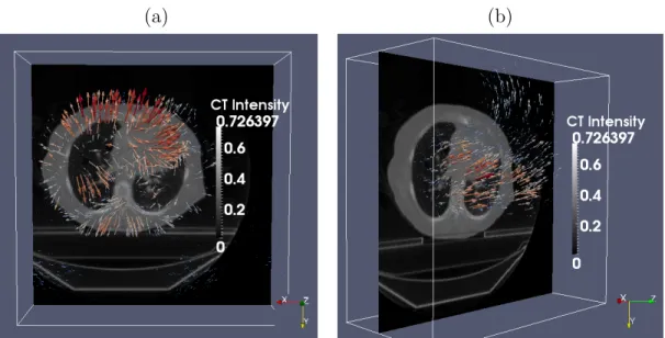
Figure 5.4.2: The (a) first and (b) second principal deformation basis functions analyzed from a lung RCCT dataset. Colored lines indicate heated body spectrum presentations of the deformation magnitudes. As shown in the images, the first principal motion consists of anterior-posterior expansion and contraction of the lung, and the second principal motion is along the superior-inferior direction. Compass in the figure: −→X : Left to Right (LR); −→Y : Anterior to Posterior (AP); −→Z : Superior to Inferior (SI).
Just prior to treatment, the Fr´echet mean image obtained at planning time is rigidly registered to the CBCT for correcting patient position. During treatment with planar imaging, CLARET iteratively applies the linear operatorsWto estimate the weightsC on the basis functions φpc from current 2D intensity residues. The residues are formed
5.5 Results
Sections 5.5.1 shows rigid registration using the NST imaging system for the head-and-neck IGRT. Section 5.5.2 shows non-rigid registration using projection images from CBCT scans acquired with the rotational imaging system for lung intra-treatment IGRT. Section 5.5.2 compares registration accuracy and efficiency of CLARET and an optimization-based approach.
5.5.1 Rigid Registration Results
CLARET’s rigid registration is tested by synthetic treatment-time projections and by real phantom projections, as described in Sections 5.5.2 and 5.5.2, respectively. The registration quality was measured by the mean absolute error (MAE) and mean target registration error (mTRE). The MAE in any of the parameters ofCis the mean, over the test cases, of the absolute error in that parameter. The mTRE for a test case is the mean displacement error, over all voxels in a 16×16×16 cm3 bounding box (the probable tumor region) centered on the pharynx in the planning CT I.
mT RE:=
Pχ
i=1(yi◦T(Ctrue)−yi◦T(Cest)) 2
χ
12
(5.5.1)
whereχis the number of pixels in the probable tumor region,yi = (y1, y2, y3) is the tuple
of theith voxel position, and C
true,Cest are the true and the estimated transformation
parameters, respectively.
Synthetic Treatment Projections
5.1.1). The target CTs were transformed from the patient’s planning CT by taking normally distributed random samples of the translation and rotation parameters within the clinical extent: ±2 cm and ±5◦, respectively. The planning CTs have a voxel size of 1.2 mm lateral, 1.2 mm anterior-posterior, and 3.0 mm superior-inferior.
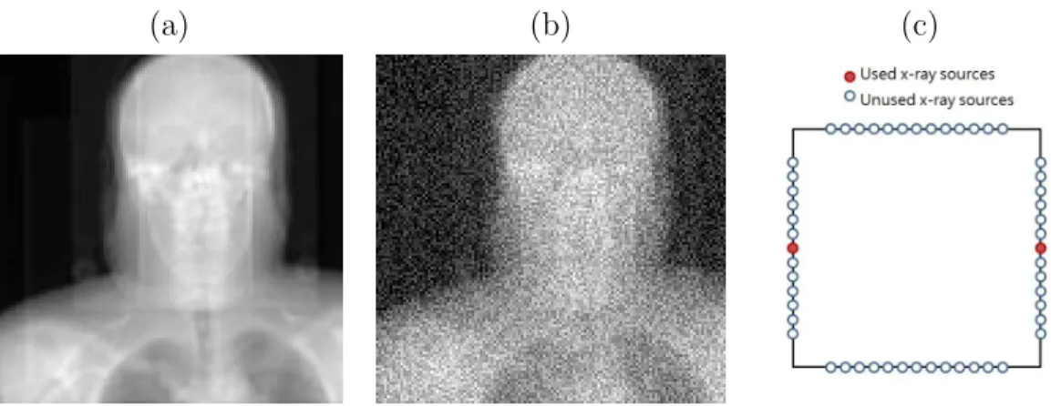
Zero mean, constant standard deviation Gaussian noise was added to the DRRs to generate the synthetic projections. The standard deviation of the noise was chosen to be 0.2 × (mean bony intensity - mean soft tissue intensity). This noise level is far higher than that produced in the NST system. An example synthetic projection is shown in Fig. 3.4.1(b).
(a) (b) (c)
Figure 5.5.1: (a) A raw DRR from a x-ray source in the NST (b) DRR with Gaussian noise added (c) the NST geometry of two opposing x-ray sources
geometry of the two opposing x-ray sources that generated the two projection images in the study. The choice of opposing sources is chosen such that the maximum angle between images ( 22.5◦) is formed with the NST system.
Figure 5.5.2: Boxplot results of errors in varying the number of projections used. Red dots are the outliers. Projections of equally spaced sources were used.
Table 7.1 shows the statistics of the errors in each rigid parameter from 90 syn-thetic test cases generated from three patients’ planning CTs (30 cases for each CT). The CLARET registration used only the two opposing NST projection images (Fig. 3.4.1(c)).
(mm; ◦) Tx Ty Tz Rx Ry Rz mTRE
MAE 0.094 0.302 0.262 0.1489 0.0248 0.1540 0.524 SE 0.008 0.022 0.075 0.011 0.001 0.030 0.076
Real Treatment Projections
CLARET’s rigid registration was also tested on a head phantom dataset. NST pro-jections (dimension: 1024×1024; pixel spacing: 0.4 mm) of the head phantom were downsampled to dimension 128×128 with a pixel spacing of 3.2 mm (Fig. 5.5.3(a)). The dimension of the planning CT is 512×512×96 with a voxel size of 3.43 mm3. The
comparison standard was obtained by rigidly registering the combined set of 52 NST projections to the planning CT by the l-BFGS optimization (Nocedal (1980)) of the similarity metric in projection space. This is not a good validation, but with no ground truths available optimization using all the projection images is our best try. Also, re-sults in Fredericket al. (2010) suggest that 2D/3D registration accuracy is higher than limted-angle-reconstructed-3D/3D registration accuracy for the NST geometry. The initial mTRE over the head region was 51.8 mm. To deal with this exceptionally large initial deviation1, CLARET trained regressions at 4 scales: W1,W2,W3, and W4. At
the sth scale of training (s = 1,2,3, and 4), each rigid parameter is collected from the combinations of E · (5−s)/4 and 0 where E ⊂ R is an extreme value selected for capturing this large setup deviation: tx, ty, tz = 80 mm; tx, ty, tz = 20 degrees.
In the registration stage the calculated multiscale linear operators are applied sequen-tially, from W1 to W4, to give new estimations of the rigid parameters from large to
small scale. The rationale behind this is that CLARET’s regression accuracy is tied to the locality of the transformation: one should learn different regressions for differ-ent transformation local neighborhoods to have more accurate estimation. For rigid registration that has to deal with a high range of patient movements, e.g., from 5 cm to 1 mm, this multi-scale learning is used to estimate parameters in a coarse-to-fine fashion. For non-rigid registration, the iterative version of CLARET did not apply this
multi-scale learning. However, later in Ch. 7 I propose a noniterative and locally-linear regression learning framework that learns more accurate regression estimators for each deformation neighborhood.
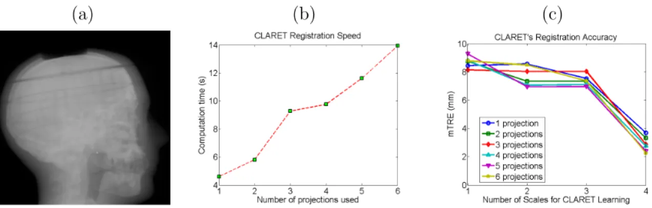
With the 4-scale training (S = 4), CLARET obtained a sub-CT-voxel mTRE of 3.32 mm using only two projections in 5.81 seconds. It was computed on a 16-core laptop GPU (NVIDIA GeForce 9400m) where the parallelization is limited. A factor of 32 speed-up (˜0.18 seconds per registration) can be expected when using a 512-core GPU. As shown in Fig. 5.5.3(b) and 5.5.3(c), CLARET accuracy improves with increased number of projections and scales in the multi-scale learning process. The registration time is approximately linear with the number of projections used.
(a) (b) (c)
Figure 5.5.3: (a) One of the test NST projections of a head phantom. (b) Time plots and (c) error plots of CLARET’s registrations on a real head-and-neck phantom dataset. Registrations were accelerated on a 16-core laptop GPU (NVIDIA GeForce 9400m).
5.5.2 Non-rigid Registration Results
mm superior-inferior) were generated with an 8-slice scanner (LightSpeed, GE Medical Systems) by acquiring multiple CT images for a complete respiratory cycle at each couch position while recording patient respiration (Real-time Position Management System, Varian Medical Systems). The CT projections were retrospectively sorted (GE Advantage 4D) to produce 3D images at 10 different respiratory phases.
Synthetic Treatment Projections
DRRs of the target CTs were used as the synthetic treatment-time projections. The DRRs were generated to simulate projections from a rotating kV imaging system (Sec-tion 3.3.1) mounted on the gantry of the medical accelerator (TrueBeam, Varian Med-ical Systems). The target CTs were deformed from the patient’s Fr´echet mean CT by taking normally distributed random samples of the coefficients of the first three PCA-derived deformation eigenmodes of the patient’s RCCT dataset (Section 4.2).
For each of the 10 CLARET registrations, I used a single simulated coronal pro-jection (dimension 128×96; pixel spacing 3.10 mm) at angle 14.18◦ (Fig. 3.4.1(d)) as input. The registration quality was then evaluated by measuring the 3D tumor centroid difference between the CLARET-estimated CT and the target CT. 3D tumor centroids were calculated from active contour (geodesic snake) segmentations (Yushkevichet al. (2006)). As shown in Table 5.2, after registration CLARET reduces the centroid error more than 85%.
Case # 1 2 3 4 5 6 7 8 9 10
Before 8.2 21.3 21.8 20.1 9.9 10.2 10.9 15.7 14.9 19.9
After 1.3 0.8 1.5 3.3 0.8 1.3 0.5 1.6 2.1 2.7
% reductions 85 96 93 84 92 87 95 90 86 86
CLARET’s registration quality was also studied in terms of average DVF (Dis-placement Vector Field) error over all cases and all CT voxels versus different angular spacings used in learning. Registrations using two projections with four different angle separations were tested by 30 randomly generated test cases. Fig. 5.5.4(a) shows that the average DVF error is small with appropriately large angular separations. How-ever, tumor motion or respiratory motion may not be visible or inferable in projections from certain angles. For example, the tumor may be obscured by denser organs (e.g., mediastinum). In Fig. 5.5.4(a) the respiration motion may not be inferable from the projection at 9.68◦ resulting in a larger error in the parameter estimation.
(a) (b)
Figure 5.5.4: Boxplots of average displacement vector field errors when varying
(a) the angular spacing and (b) the number of projections used for CLARET’s non-rigid registration. Red dots are the outliers. In (a), two projections for each test were used. For the zero-degree test case, only one projection was used. In (b), DRRs spanning 9.68◦ about 14.18◦ were used in each test. The single projection was tested at 14.18◦ (see Fig. 3.4.1(d)).
Real Treatment Projections
in the 2D/3D registration. The RMS window width was set to 32.0 mm for the Gaus-sian normalization for this imaging geometry, which was predetermined to yield the smallest 3D centroid error in one lung dataset (Fig. 5.5.5). Future studies should check whether this window size is also best for other datasets.
Figure 5.5.5: 3D tumor centroid error plots on a lung dataset for varying width of the Gaussian window used for CLARET’s local Gaussian normalization.
The results shown in Table 5.3 suggest a consistency in registration quality between the synthetic image tests and real projection image tests. The mean and standard deviation of 3D tumor centroid errors following 2D/3D registration are 2.66 mm and 1.04 mm, respectively.2 The average computation time is 2.61 seconds on a 128-core GPU, NVIDIA GeForce 9800 GTX. A factor of four speed-up (to 0.65 seconds) can be expected when using a 512-core GPU for acceleration.
The clinical goal is to improve tumor localization during treatment using CLARET. Assuming a mean lung tumor motion extent of about 10 mm, the standard deviation is about one-third of the motion extent, or 3 mm. In order to improve on current clinical practice (i.e., no image guidance during treatment) an mTRE of 2 mm or less is
2The errors include an uncertainty in tumor position in the CBCT projections, owing to variability
desirable. Furthermore, since most of the motion is in the superior-inferior direction, it is desirable to achieve an mTRE of 2 mm or less in that direction. Our results show that CLARET achieves the clinically desired accuracy: the mean and standard deviation of the 2D tumor centroid error on the patient plane (left-right and superior-inferior directions) after registration is 1.96 mm and 1.04 mm, respectively. CLARET reduces positional errors in directions along the plane of the projection more than in the out-of-plane direction. As shown in Table 5.3, except in cases from patient #1 most of the percent 2D error reductions in the imaging plane (which was coronal) are larger than the percent error reductions in the out-of-plane direction. This is expected because 2D/3D registration with a single projection is more sensitive to tumor displacements in the image plane but less sensitive to scale changes due to out-of-plane displacements.
P atien t # e 3 D E E (mm) e 2 D E E (mm) e
⊥ EE
(mm) e 3 D E I (mm) e 2 D E I (mm) e
⊥ EI
(a) (b)
(a) (b) (c)
Figure 5.5.7: The same 3-space lines in (a) the mean CT, (b) the reconstructed CBCT at the EE phase and (c) the estimated CT of the same lung dataset used in figure 5.5.6(b). Upper row: lines indicate the tumor centroid in the CBCT at the EE phase; lower row: lines indicate the diaphragm contour in the CBCT at the EE phase.
Comparison to an Optimization-based Registration Method
for the projection operator P, and the same testing datasets.3
For the comparisons, 30 randomly sampled synthetic deformations were used as the test cases for each of the five lung patients. The deformations were sampled randomly within ±3 standard deviations of deformations observed in the patient’s RCCT. For each test case, a single coronal CBCT projection (dimension: 1024×768 downsampled to dimension: 128×96) was simulated from the deformed Fr´echet mean CT as the target projection. Both methods were initialized with the realistic Fr´echet mean image with no deformation: C(0) =ˆ 0 in Eq. 5.1.2.
For CLARET, each training deformation parameter ci (i = 1,2,3) was collected from the combinations of ±3σi, ±1.5σi, and 0 where σi is the standard deviation of
the ith eigenmode weights observed in the patient’s RCCT. Therefore, for sampling on
three eigenmodes, a total of 125 training deformations are sampled for each patient. Registration accuracy was measured by the average registration error distance over the lung region. As Fig. 5.5.8 shows, CLARET yielded more accurate results than the l-BFGS optimization-based registration in almost every test case in all five patients. Table 5.4 showed statistical comparisons of the registration accuracy. The maximum error produced by CLARET among the 30×5=150 test cases is only 0.08 mm where the maximum error produced by l-BFGS is 13.15 mm, which is 164 times higher than CLARET. The smaller median error and error standard deviation also showed that CLARET is more accurate and more robust than the l-BFGS optimization-based ap-proach.4
In term of registration speed, Fig. 5.5.9 showed that CLARET is faster than l-BFGS in every test case and has relatively small variation in speed. The statistical results
3Despite this my implementation is not completely the same as the method in Liet al.(2011a), but
I had no access to the implementation in Liet al. (2011a).
4Note that the l-BFGS optimization-based approach also yields accurate registration with a mean
shown in Table 5.5 indicate that the longest registration time produced by CLARET is still shorter than the shortest time produced by l-BFGS.
As our results show, in my implementations CLARET is more robust, accurate, and faster than the l-BFGS optimization.
mTRE (mm) min. max. median mean std
CLARET 1.1e−5 0.08 2.3e−4 1.5e−3 7.4e−3
l-BFGS 2.0e−4 13.15 8.8e−3 0.54 2.01
Table 5.4: Registration accuracy (mTRE) statistics on the five patient data: CLARET vs. the l-BFGS optimization. std=standard deviation
time (s) min. max. median mean std
CLARET 0.94 5.15 1.73 1.95 0.74 l-BFGS 5.29 78.73 19.30 23.76 14.41
Chapter 6: Nonlinear Regression Learning
In this chapter, I present another 2D/3D registration method that relaxes the strong linear assumption made in CLARET. It uses a nonlinear neighborhood analysis ap-proach and calculates the patient’s treatment-time 3D deformations by kernel regres-sion. The method is called Registration Efficiency and Accuracy through Learning Metric on Shape (REALMS). Specifically, each of the patient’s deformation param-eters is interpolated using a weighting Gaussian kernel on that parameter’s training case values. In each training case, its parameter value is associated with a correspond-ing traincorrespond-ing projection image. The Gaussian kernel is formed from distances between training projection images. This distance for the parameter in question involves a Rie-mannian metric on projection image differences. At planning time, REALMS learns the parameter-specific metrics from the set of training projection images using a Leave-One-Out (LOO) training that best fits to the training set.
The rest of the chapter is organized as follows: in Section 6.1, I describe REALMS’s novel registration scheme that uses kernel regression. In Section 6.2, I describe the metric learning scheme and the specialized initialization in REALMS. I show synthetic and real results in Section 6.3.
6.1 2D/3D Registration Framework
This section details REALMS’s 2D/3D registration framework. REALMS uses kernel regression (Eq. 6.1.1) to interpolate the patient’s n 3D deformation parameters
C= (c1, c2,· · · , cn) separately from the on-board projection image Ψ(θ) where θ is the projection angle. It uses a Gaussian kernelKMi,σi with widthσi and a metric tensorMi
on projection intensity differences to interpolate the patient’sithdeformation parameter
ci from a set of N training projection images {P(I◦T(C
κ);θ)|κ= 1,2,· · · , N}
sim-ulated at planning time. Specifically, the training projection image, P(I◦T(Cκ);θ),
is the DRR of a 3D image deformed from the patient’s planning-time 3D mean im-age I with sampled deformation parameters Cκ = (c1κ, cκ2,· · · , cnκ). T and P are the
warping and the DRR operators, respectively. Psimulates the DRRs according to the treatment-time imaging geometry, e.g., the projection angle θ.
In the treatment-time registration, each deformation parameter ci in C can be
interpolated with the following kernel regression:
ci =
N
P
κ=1
ciκ·KMi,σi(Ψ(θ),P(I◦T(Cκ);θ))
N
P
κ=1
KMi,σi(Ψ(θ),P(I◦T(Cκ);θ))
, (6.1.1)
KMi,σi(Ψ(θ),P(I◦T(Cκ);θ)) =
1
√
2πσie
−d 2
Mi(Ψ(θ),P(I◦T(Cκ);θ))
d2Mi(Ψ(θ),P(I◦T(Cκ);θ)) = (Ψ(θ)−P(I◦T(Cκ);θ))|Mi(Ψ(θ)−P(I◦T(Cκ);θ)),
(6.1.3) where KMi,σi is a Gaussian kernel (kernel width= σi) that uses a Riemannian metric
Mi in the squared distanced2Mi and gives the weights for the parameter interpolation in
the regression. The minus signs in Eq. 6.1.3 denote pixel-by-pixel intensity subtraction. REALMS uses the same deformation space parameterization as CLARET’s (See Section 4.2). In the next section, I describe how it learns the metric tensor Mi and
decides the kernel width σi.
6.2 Metric Learning at Planning Time
6.2.1 Metric Learning and Kernel Width Selection
REALMS learns a metric tensor Mi ⊂ RP×P with a corresponding kernel width σi
for the patient’s ith deformation parameter ci using a Leave-One-Out (LOO) train-ing strategy. At planntrain-ing time, it samples a set of N deformation parameter tuples
{Cκ = (c1κ, c2κ,· · · , cnκ)|κ= 1,2,· · ·N} to generate training projection images
{P(I◦T(Cκ);θ)|κ= 1,2,· · · , N} where their associated deformation parameters are
sampled uniformly within three standard deviations of the scores λτ observed in the
RCCT. For each deformation parameter ci in C, REALMS finds the best pair of the metric tensor Mi† and the kernel width σi† that minimizes the sum of squared LOO regression residualsLci among the set of N training projection images:
Mi†, σi†= arg Mi,σi
Lci(Mi, σi) =
N
X
κ=1
ciκ−cˆi κ(M
i
, σi) 2 , (6.2.2) ˆ ci κ(M i
, σi) = P
χ6=κ
ciχ·KMi,σi(P(I◦T(Cκ);θ),P(I◦T(Cχ);θ))
P
χ6=κ
KMi,σi(P(I ◦T(Cκ);θ),P(I ◦T(Cχ);θ))
, (6.2.3)
where ˆci
κ(Mi, σi) is the estimated value for parameter ciκ interpolated by the metric
tensor Mi and the kernel width σi from the training projection images χ other than
κ; Mi needs to be a positive semi-definite (p.s.d) matrix to fulfill the pseudo-metric constraint; and the kernel width σi needs to be a positive real number.
To avoid high-dimensional optimization over the constrained matrixMi, I structure
the metric tensorMi as a rank-1 matrix formed by a basis vector ai ⊂ RP×1:
Mi =aiai| (6.2.4)
Therefore, we can transform Eq. 6.2.1 into an optimization over the unit vector ai wherekaik2 = 1:
ai†, σi†=arg ai,σi
minLci(aiai|, σi) (6.2.5)
Then we can rewrite the squared distance d2
Mi =d2aiai| used in the Gaussian kernel
KMi,σi as follows:
d2aiai|(P(I◦T(Cκ);θ),P(I◦T(Cχ);θ)) = (ai|·rκ,χ)|(ai|·rκ,χ), (6.2.6)
rκ,χ =P(I◦T(Cκ);θ)−P(I◦T(Cχ);θ), (6.2.7)
images generated by parametersCκ and Cχ; and ai is a metric basis vector where the
magnitude of the inner product of ai and the intensity difference vector rκ,χ, ai|·rκ,χ
gives the distance for the parameterci (Eq. 6.2.6).
The learned metric basis vectorai†and the selected kernel widthσi†form a weighting
kernelKai†ai†|,σi† to interpolate the parameterci in the registration (see Eq. 6.1.1).
6.2.2 Linear-Regression Implied Initial Metric
Since the residual functionalL(see Eq. 6.2.1) that we want to minimize is non-convex, a good initial guess of the metric basis vector a is essential. Therefore, REALMS uses a vector wi as an initial guess of the metric basis vector ai for the parameter ci.
Let W ⊂ RP×n =
w1 w2 · · · wn
list these initial guesses. The matrix W is approximated by a multivariate linear regression (Eq. 6.2.8 and Eq. 6.2.9) between the projection difference matrix R ⊂RN×P = (r
1r2· · ·rN)| and the parameter differences
matrix ∆C. In particular, the projection difference vectorrκ =P(I◦T(Cκ);θ)−P(I;θ)
is the intensity differences between the DRRs calculated from the deformed image
I◦T(Cκ) and the DRRs calculated from the mean image I (where C=0).
∆C=
c11 c21 · · · cn1
c12 c22 · · · cn2
..
. ... . .. ...
c1
N c2N · · · cnN
−0≈
r|1 r|2 .. . r|N
·
w1 w2 · · · wn
=W|R (6.2.8)
W= (R|R)−1R|∆C (6.2.9)
This is just the regression that was used to train CLARET.