How do individual-level sociodemographics and
neighbourhood-level characteristics in
fl
uence
residential location behaviour in the context of the
food and built environment? Findings from 25 years
of follow-up in the CARDIA Study
Pasquale E Rummo,
1David K Guilkey,
2James M Shikany,
3Jared P Reis,
4Penny Gordon-Larsen
1▸Additional material is published online only. To view please visit the journal online (http://dx.doi.org/10.1136/jech-2016-207249).
1Department of Nutrition,
Gillings School of Global Public Health, University of North Carolina at Chapel Hill, Carolina Population Center, Chapel Hill, North Carolina, USA
2
Department of Economics, University of North Carolina at Chapel Hill, Carolina Population Center, Chapel Hill, North Carolina, USA
3Division of Preventive
Medicine, University of Alabama at Birmingham, Birmingham, Alabama, USA
4Division of Cardiovascular
Sciences, National Heart, Lung, and Blood Institute, Bethesda, Maryland, USA
Correspondence to Dr Penny Gordon-Larsen, Department of Nutrition, Gillings School of Global Public Health, University of North Carolina, USA; pglarsen@unc. edu
Received 22 January 2016 Revised 16 August 2016 Accepted 26 August 2016 Published Online First 21 September 2016
To cite:Rummo PE, Guilkey DK, Shikany JM,
et al.J Epidemiol Community Health
2017;71:261–268.
ABSTRACT
Background Little is known about how diet-related and activity-related amenities relate to residential location behaviour. Understanding these relationships is essential for addressing residential self-selection bias.
Methods Using 25 years (6 examinations) of data from the Coronary Artery Risk Development in Young Adults (CARDIA) study (n=11 013 observations) and linked neighbourhood-level data from the 4 CARDIA baseline cities (Birmingham, Alabama; Chicago, Illinois; Minneapolis, Minnesota; Oakland, California, USA), we characterised participants’neighbourhoods as having low, average or high road connectivity and amenities using non-hierarchical cluster analysis. We then used repeated measures multinomial logistic regression with random effects to examine the associations between individual-level sociodemographics and neighbourhood-level characteristics with residential neighbourhood types over the 25-year period, and whether these associations differed by individual-level income.
Results Being female was positively associated with living in neighbourhoods with low (vs high) road connectivity and activity-related and diet-related amenities among high-income individuals only. At all income levels, a higher percentage of neighbourhood white population and neighbourhood population <18 years were associated with living in neighbourhoods with low (vs high) connectivity and amenities. Individual-level race; age; and educational attainment,
neighbourhood socioeconomic status and housing prices did not influence residential location behaviour related to neighbourhood connectivity and amenities at any income level.
Conclusions Neighbourhood-level factors appeared to play a comparatively greater role in shaping residential location behaviour than individual-level
sociodemographics. Our study is an important step in understanding how residential locational behaviour relates to amenities and physical activity opportunities, and may help mitigate residential self-selection bias in built environment studies.
BACKGROUND
A primary challenge of neighbourhood health research is that it is difficult to tease apart the infl u-ence of the neighbourhood on its residents from the fact that residents locate in neighbourhoods on the basis of health-related amenities. If
unaccounted for, neighbourhood selection factors may bias associations of built environment factors and health outcomes.1Therefore, to address
poten-tial residenpoten-tial self-selection bias, it is important to understand how access to health-related amenities influences residential behaviour.
The few studies that have addressed how diet-related and activity-related amenities relate to residential location behaviour have found a positive association between residential location with prox-imity and number of retail and physical activity (PA) facilities.2–4 There are also examples of self-reported preferences for living in neighbourhoods with lower intersection density and street net-works,3 5 6 despite positive observed associations
between road connectivity and PA.7
Furthermore, there is evidence to support that individuals’self-reported residential preferences are influenced by individual-level sociodemographics and neighbourhood characteristics, such as proxim-ity to employment subcentres and accessibilproxim-ity of parks.8–14However, these studies largely lack time-varying data and examine residential preferences (vs actual location behaviour), with limited geographic generalisability. Little is known about how the rela-tionship between diet-related and activity-related amenities and residential location behaviour varies by individual-level income.
Using 25 years of time-varying data from the Coronary Artery Risk Development in Young Adults (CARDIA) study with linked neighbourhood-level data from four US cities, we sought tofill these gaps. We used repeated measures to estimate average asso-ciations between individual-level sociodemographics and neighbourhood-level characteristics of CARDIA participants with neighbourhood diet-related and activity-related amenities and infrastructure over time. Since income is a major factor in residential location behaviour,5 we hypothesised that these
associations would differ by individual-level income.
METHODS Study sample
Alabama; Chicago, Illinois; Minneapolis, Minnesota; Oakland, California, USA), with approximately equal enrolment by age (18–24, 25–30 years), race (black, white), gender and education (high school or less, more than high school). Follow-up exami-nations were conducted in 1987–1988 (year 2), 1990–1991 (year 5), 1992–1993 (year 7), 1995–1996 (year 10), 2000– 2001 (year 15), 2005–2006 (year 20) and 2010–2011 (year 25), with participant retention of 91%, 86%, 81%, 79%, 74%, 72% and 72%, respectively. We used a restricted sample of CARDIA participants who remained in (or returned to) the four baseline cities at any given examination year (n=12 308 person-observations), for a total of 4316, 2462, 1728, 1481, 1202 and 1119 participants at baseline and examination years 7, 10, 15, 20 and 25, respectively. Compared with the full CARDIA sample, individuals in our analytic sample (ie, living in one of the four cities at each examination year) were younger and less white and there was a greater proportion of male participants.
Residential locations of participants were determined from geocoded home addresses at each examination year. We defined neighbourhoods using real estate-derived boundaries from Zillow15where available (Chicago, Illinois; Oakland, California;
Minneapolis, Minnesota, USA) and the Regional Planning Commission of Greater Birmingham (Birmingham, Alabama, USA; n=392 neighbourhoods at each examination year). Using a Geographic Information System (GIS), we geographically and temporally matched neighbourhood-level data to participants’ residential locations. Neighbourhood features 23 m along the boundaries of adjacent neighbourhoods were assigned to each adjacent neighbourhood since they would theoretically be prox-imate to each other.
Cluster analysis to derive neighbourhood types
Our baseline sample of CARDIA individuals was geographically clustered due to targeted enrolment by age, gender, race and education, thus there were neighbourhoods in the four cities with zero or few participants. Therefore, we createda posteriori neighbourhood clusters using non-hierarchical cluster analysis to characterise neighbourhoods where sufficient numbers of indivi-duals lived.
Since we were interested in understanding relationships between residential location behaviour and physical environment in the context of residential self-selection bias,1 we sought to capture neighbourhood characteristics related to diet and PA. Specifically, we used variables related to the count of food outlets and PA facilities ( per km2), distance from participants’residence
to the nearest employment centre centroid, road types and lengths, and total park area (km2) within each neighbourhood at
each examination year (see online supplementary file 1).16 Theoretically, the distribution of these variables shapes diet beha-viours and/or PA opportunities.7 8 17 18
We transformed all calculated variables used to define neigh-bourhood clusters into z-scores by examination year and city to achieve comparability across measures. Then using the PROC FASTCLUS procedure in SAS (V.9.3), we conducted cluster ana-lyses using means of these standardised variables at each exam-ination year and a range of 2–6 clusters. To determine afinal cluster solution, we evaluated the distribution of individuals across clusters; differences in proportions across clusters; parsi-mony and meaningfulness of clusters. We classified values≥0.5 or ≤−0.50 as high or low, respectively.19 We also evaluated whether clusters appeared repeatedly across solutions (robust-ness) by performing the cluster analysis many times. After deter-mining the appropriate number of clusters from this step, we
performed 1000 iterations of the cluster analysis using a SAS macro, which identified the cluster solution with the highest R2
value; we used this categorical variable of neighbourhood type as our outcome.
Neighbourhood-level exposures
We adjusted for several neighbourhood-level sociodemographic confounders. We obtained data related to neighbourhood-level socioeconomic status (SES), racial composition, age structure and rental properties at the census tract level from the USA. US Census 1980, 1990, and 2000 and American Community Survey 5-year estimates from 2005 to 2009 and 2007 to 2011 (when comparable US Census data were unavailable). Using linear interpolation, we estimated a continuous change in socio-demographic characteristics across the full period of the decen-nial and quinquennial censuses. We also derived a neighbourhood socioeconomic deprivation score using principal components analysis of: (1) percentage of population with less than high school education at age 25; (2) percentage of popula-tion with at least a college degree at age 25; (3) median house-hold income and (4) percentage of population with househouse-hold income <150% of federal poverty level;20a higher score
indi-cates higher neighbourhood socioeconomic deprivation. We calculated the average of quarterly values for home price index (HPI) in each city at each examination year using values from Moody’s Analytics.21 Moody’s provides Case-Schiller
price data for Chicago, Minneapolis and Oakland for each quarter of each year from 1975 to 2012 relative to a value of 100 for the first quarter of the year 2000. Moody’s provides Lender Processing Service data for Birmingham at the zip code level for each quarter from 1991 to 2012, measured in the thousands of dollars. We used multilevel mixed-effects linear regression (-mixed- in Stata V.13.0) to predict HPI values for 1985 in Birmingham (see online supplementaryfile 1).
Given that neighbourhood-level variables were available at different geographic levels, we harmonised all variables (includ-ing those used to define neighbourhood cluster types) tofit our socially constructed neighbourhood boundaries within city limits. We also created a geographically weighted estimate of neighbourhood-level variables when data source boundaries did not align with neighbourhood boundaries (assuming an equal distribution within source boundaries).
Individual-level exposures
We also adjusted for several individual-level sociodemographic confounders. At each CARDIA examination year, a standardised questionnaire was used to collect self-reported individual-level sociodemographic characteristics, including age, gender, race and current educational attainment (highest grade or year of school completed). Income was collected with categorical responses at examination years 5, 7, 10, 15, 20 and 25; we sub-stituted income values from examination year 5 for baseline values, which were unavailable.
Statistical analysis
Our individual-level exposures included age (continuous), race (black, white), gender and education (high school or less, more than high school); and our neighbourhood-level exposures included socioeconomic deprivation score, percentage of non-Hispanic white population, percentage of the population
≤18 years and the percentage of neighbourhood rental proper-ties (occupied and vacant). We also adjusted for neighbourhood land area, examination year and study centre. Based on evidence showing that model estimates may improve with interaction terms for income groups,12we stratified our analyses by tertiles
of individual-level income (coded as the midpoint of the cat-egorical response).
We used Stata (V.13.0) for all analyses (-mlogit-) with the -suest- postestimation command to obtain a joint covariance matrix for all estimated coefficients. Then we used the -test-command to determine whether coefficients (ie, estimated effect of exposures on the probability of residing in each neighbour-hood type) were equal across tertiles of individual-level income. We accounted for clustering by neighbourhood ID using the
‘cluster’option.
To quantify changes in the neighbourhood type in response to changes in each exposure, we used the -margins- postestima-tion command with the -predict- oppostestima-tion to predict the probabil-ity of residing in each neighbourhood type atfixed levels of the covariates (categories or ±1SD of mean) within each income tertile.
To account for potential selection bias due to out-migration from the four cities over time, we used a probit model to derive inverse probability weights. We used gender, race and baseline study centre to predict the probability of being in the sample at year 25, and used the inverse of the probability to weight the models in the central analysis (-pweight-).
Given empirical evidence of the importance of housing price in residential behaviour,12we ran two separate models: a model
with neighbourhood clusters stratified by high and low HPI (<50th and≥50th centile, respectively) and a model with non-stratified clusters. We used a likelihood-ratio test to assess thefit of these two models.
RESULTS
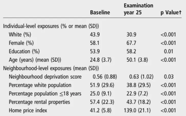
Compared with baseline, the analytic sample at the end of follow-up was less white, older and more educated, with a greater proportion of female participants (table 1).
Ourfinal cluster solution included three distinct clusters, with 545 (23.2%), 409 (17.4%) and 1398 (59.4%) neighbourhoods assigned to clusters with low, average, and high road connectiv-ity and activconnectiv-ity-related and diet-related amenities, respectively (see online supplementaryfile 2). The low cluster type was char-acterised by a higher total road length, park area and count of cul-de-sacs, with greater distance to employment subcentres; lower intersection density and a lower count of PA facilities and convenience stores (see online supplementaryfile 3). In contrast, the high cluster had a higher intersection density, count of road links and β-index, with a higher count of PA facilities and all food outlets; a lower percentage of local roads and closer prox-imity to employment subcentres. The fit of the model with fewer clusters was statistically significantly better than the model with clusters divided by high/low HPI ( p<0.05); thus, we included HPI as a covariate rather than stratify clusters in the
final model.
Across all tertiles of individual-level income, individual-level race, educational attainment and age were not statistically signifi -cantly associated with any of our derived residential clusters over time (table 2). Whereas, the probability of residing in a
neighbourhood with low (vs high) road connectivity and activity-related and diet-related amenities was higher for females (vs males) within the high-income tertile only (table 3).
At all levels of individual-level income, the probability of res-iding in a neighbourhood with low (vs high) amenities/connect-ivity increased as the percentage of neighbourhood white population increased and as the percentage of neighbourhood population≤18 years increased. Regardless of income level, we did not observe statistically significant associations between neighbourhood socioeconomic deprivation and HPI with resi-dential neighbourhood type. However, the probability of resid-ing in the low (vs high) amenities/connectivity neighbourhood type decreased as the percentage of rental housing units increased for all participants.
Overall,findings for medium-income participants were similar to low-income participants (relative to high-income participants). However, the probability of residing in the low (vs high) connect-ivity/amenities neighbourhood type was not statistically signifi -cantly associated with the percentage of neighbourhood white population among medium-income participants.
DISCUSSION
Using 25 years of retail and built environment data, we exam-ined relationships between individual-level sociodemographics and neighbourhood-level characteristics with living in activity-supportive, commercially dense neighbourhoods over time, and whether these associations differed by individual-level income. We found that individual-level race, age, and educational attain-ment, and neighbourhood SES and housing prices were not associated with residential location over time whereas, individual-level gender was a significant predictor of neighbour-hood residential type among high-income CARDIA participants only. Neighbourhood racial and age composition and percentage of rental properties were also related to residential location behaviour at all income levels.
Although previous literature suggests that individual-level race, age and educational attainment influence residential prefer-ences,12 13 17 22 we did not observe similar findings with
Table 1 Descriptive statistics of analytic and CARDIA sample* across follow-up (1985/1986–2010/2011)
Baseline
Examination
year 25 p Value†
Individual-level exposures (% or mean (SD))
White (%) 43.9 30.9 <0.001 Female (%) 58.1 67.7 <0.001 Education (%) 53.9 58.2 0.01 Age (years) (mean (SD)) 24.8 (3.7) 50.1 (3.8) <0.001 Neighbourhood-level exposures (mean (SD))
Neighbourhood deprivation score 0.56 (0.88) 0.63 (1.02) 0.03 Percentage white population 51.9 (29.6) 38.8 (29.5) <0.001 Percentage population≤18 years 25.0 (9.1) 22.9 (7.2) <0.001 Percentage rental properties 57.4 (22.3) 43.7 (18.2) <0.001 Home price index 41.2 (5.8) 139.0 (21.1) <0.001
*The analytic sample only included participants who remained in the four baseline CARDIA cities at any given examination year, with a total of 4314, 2461, 1727, 1480, 1202 and 1119 participants at baseline and examination years 7, 10, 15, 20 and 25, respectively.
†One-way ANOVA was used to test whether the difference between values at baseline and examination year 25 was statistically significantly different from one another.
Table 2 Multivariable-adjusted†β-coefficients (95% CI) of association between individual-level sociodemographics and neighbourhood-level characteristics (exposures) and low, average and high neighbourhood cluster type‡by income status using multivariate multinomial logistic regression, CARDIA examination years 0–25
Low connectivity/amenities (n=545 (23.2%))
p for equality of coefficients (low vs high income)§
Average connectivity/ amenities (n=409 (17.4%))
p for equality of coefficients (average vs high income)§
High connectivity/ amenities (n=1398 (59.4%))
Low income (first tertile)
White¶ −0.13 (−0.65 to 0.40) 0.29 0.16 (−0.28 to 0.59) 0.05 1.00 Female −0.07 (−0.39 to 0.26) 0.0001 −0.11 (−0.39 to 0.17) 0.09 1.00 Education** −0.26 (−0.54 to 0.02) 0.14 −0.20 (−0.42 to 0.03) 0.45 1.00 Age (years) 0.03 (0.01 to 0.07) 0.16 0.01 (−0.03 to 0.04) 0.15 1.00 Neighbourhood deprivation score −0.24 (−0.71 to 0.23) 0.14 −0.05 (−0.49 to 0.40) <0.001 1.00 Percentage white population 0.01 (−0.0002 to 0.03)* 0.36 0.01 (−0.004 to 0.02) 0.002 1.00 Percentage population≤18 years 0.10 (0.07 to 0.14)* 0.25 0.07 (0.04 to 0.10)* 0.48 1.00 Percentage rental properties −0.03 (−0.04 to−0.01)* 0.10 −0.02 (−0.04 to−0.01)* 0.80 1.00 Home price index −0.002 (−0.01 to 0.01) 0.15 0.003 (−0.005 to 0.01) 0.12 1.00 Neighbourhood land area 0.35 (0.26 to 0.44)* 0.11 −0.10 (−0.20 to−0.01)* 0.03 1.00 Examination year
Year 0 0.00 − 0.00 − 1.00
Year 7 −0.46 (−1.02 to 0.10) 0.14 −0.32 (−0.81 to 0.16) 0.46 1.00 Year 10 −0.14 (−0.79 to 0.51) 0.89 −0.26 (−0.80 to 0.29) 0.81 1.00 Year 15 −0.15 (−1.05 to 0.76) 0.63 −0.35 (−1.14 to 0.43) 0.94 1.00 Year 20 −0.26 (−1.77 to 1.26) 0.33 −0.40 (−1.60 to 0.81) 0.37 1.00 Year 25 −0.34 (−1.68 to 0.99) 0.68 −0.42 (−1.47 to 0.63) 0.76 1.00 Baseline city††
Birmingham 1.38 (0.25 to 2.52)* 0.45 −0.31 (−1.20 to 0.59) 0.13 1.00
Chicago − − 1.00
Minneapolis 3.40 (2.02 to 4.77)* 0.97 0.67 (−0.49 to 1.84) 0.21 1.00 Oakland 3.52 (2.04 to 5.00)* 0.97 0.56 (−0.66 to 1.79) 0.57 1.00 Medium income (second tertile)
White¶ 0.04 (−0.72 to 0.81) 0.16 0.30 (−0.10 to 0.71) 0.10 1.00 Female −0.02 (−0.43 to 0.39) 0.0001 0.01 (−0.34 to 0.36) 0.20 1.00 Education** −0.40 (−0.81 to 0.02) 0.07 −0.31 (−0.64 to 0.03) 0.30 1.00 Age (years) 0.01 (−0.04 to 0.07) 0.20 0.02 (−0.02 to 0.06) 0.08 1.00 Neighbourhood deprivation score −0.28 (−0.79 to 0.23) 0.10 0.16 (−0.34 to 0.66) 0.001 1.00 Percentage white population 0.01 (−0.01 to 0.02) 0.15 0.01 (−0.01 to 0.03) 0.01 1.00 Percentage population≤18 years 0.12 (0.07 to 0.17)* 0.42 0.08 (0.05 to 0.12)* 0.65 1.00 Percentage rental properties −0.04 (−0.06 to−0.02)* 0.04 −0.04 (−0.05 to−0.02)* 0.32 1.00 Home price index 0.0002 (−0.01 to 0.01) 0.20 0.003 (−0.01 to 0.01) 0.14 1.00 Neighbourhood land area 0.36 (0.24 to 0.47)* 0.01 −0.12 (−0.21 to−0.03)* 0.03 1.00 Examination year
Year 0 0.00 − 0.00 − 1.00
Year 7 0.07 (−0.69 to 0.83) 0.77 −0.23 (−0.86 to 0.39) 0.61 1.00 Year 10 −0.16 (−1.14 to 0.81) 0.92 −0.49 (−1.29 to 0.32) 0.49 1.00 Year 15 −0.23 (−1.53 to 1.06) 0.71 −0.52 (−1.62 to 0.59) 0.90 1.00 Year 20 −0.89 (−3.10 to 1.31) 0.60 −0.89 (−2.67 to 0.88) 0.56 1.00 Year 25 −0.74 (−2.68 to 1.19) 0.91 −1.24 (−2.84 to 0.36) 0.70 1.00 Baseline city††
Birmingham 1.37 (0.0003 to 2.74)* 0.38 −0.58 (−1.39 to 0.24) 0.36 1.00
Chicago 0.00 − 0.00 − 1.00
Minneapolis 3.66 (2.17 to 5.16)* 0.76 0.21 (−0.74 to 1.15) 0.70 1.00 Oakland 4.18 (2.44 to 5.93)* 0.44 0.67 (−0.41 to 1.75) 0.44 1.00 High income (third tertile)
White ¶ −0.68 (−1.56 to 0.20) − −0.63 (−1.26 to 0.0001) − 1.00 Female 1.07 (0.59 to 1.54)* − 0.33 (−0.11 to 0.77) − 1.00 Education** 0.29 (−0.37 to 0.96) − 0.09 (−0.60 to 0.78) − 1.00 Age (year) −0.05 (−0.14 to 0.05) − −0.05 (−0.12 to 0.02) − 1.00 Neighbourhood deprivation score 0.21 (−0.36 to 0.77) − 1.04 (0.45 to 1.63)* − 1.00 Percentage white population 0.03 (−0.0003 to 0.05)* − 0.03 (0.02 to 0.05)* − 1.00 Percentage population≤18 years 0.16 (0.07 to 0.25)* − 0.10 (0.02 to 0.18)* − 1.00
objectively measured residential location in our study across follow-up. These inconsistencies may be due to the use of pref-erence data in previous studies, which assumes that prefpref-erence measures capture true preferences and residential movement.1
We also found that high-income female participants were more likely to reside in areas with low (vs high) connectivity/amen-ities, but we did not observe similar associations among low-income or medium-low-income female participants. Although research indicates that women prefer to live in more compact neighbourhoods,13 high-income women may be able to afford
to own a car and drive to destinations, and thus may have suffi -cient income to choose to reside in less urban areas.23
Participants of all income levels were more likely to reside in neighbourhoods with low (vs high) connectivity/amenities as the percentage of population <18 years increased. This finding is supported by several studies showing that households with school-age children tend to live in less densely populated, subur-ban areas,14 22and prefer to locate near other households with
families.12 Those with families may also seek larger houses, which tend to be more affordable in suburban (vs urban) areas. Similarly, the percentage of neighbourhood white population was positively associated with locating in neighbourhoods with low (vs high) connectivity/amenities. This finding is consistent with previous work indicating that suburban white households tend to be located in neighbourhoods with better conditions (eg, fewer abandoned buildings).24
Finally, we found that housing price was not related to resi-dential neighbourhood type at any income level, but the per-centage of rental housing units was negatively associated with the locating in neighbourhoods with low (vs high) amenities
and connectivity. Although the latter is consistent with research showing that renters are less likely to live in less commercial, suburban neighbourhoods,22 we expected lower income indivi-duals to be more sensitive to housing prices11and to locate near
amenities if housing was more affordable. However, our indices did not include prices of apartments or multifamily dwellings,21
and thus may not have accurately reflected the housing market for low-income individuals.
Based on these preferences, our findings also suggest that residential location behaviour may bias estimates of the rela-tionship between the physical environment and health out-comes. Hypothetically, individuals living in neighbourhoods with greater PA opportunities are more likely to be physically active, and individuals who live in areas with a high density of eating-out options may have poorer dietary behaviours. Therefore, future studies should employ methodological approaches, such as statistical control and complex economet-ric approaches,25 to account for these potential sources of
bias.
Studies that examine the influence of the food and built environment on residential location behaviour are mostly based on self-reported preference surveys2 26 and
cross-sectional data.2 26 27 In contrast, we had access to detailed, time-varying measures, which allowed us to use information both within and between participants, thus producing more efficient results and reducing measurement error. We used actual residential location data versus preferences, the latter of which is subject to social desirability bias.28 Our cluster
ana-lysis approach also provided distinct, robust and meaningful groups of neighbourhood types, which may be generalisable
Table 2 Continued
Low connectivity/amenities (n=545 (23.2%))
p for equality of coefficients (low vs high income)§
Average connectivity/ amenities (n=409 (17.4%))
p for equality of coefficients (average vs high income)§
High connectivity/ amenities (n=1398 (59.4%))
Percentage rental properties −0.04 (−0.07 to−0.02)* − −0.05 (−0.07 to−0.02)* − 1.00 Home price index 0.01 (−0.01 to 0.035) − 0.02 (0.0003 to 0.03)* − 1.00 Neighbourhood land area 0.22 (0.08 to 0.36)* − −0.27 (−0.43 to−0.11)* − 1.00 Examination year
Year 0 0.00 − 0.00 − 1.00
Year 7 0.22 (−0.62 to 1.05) − −0.02 (−0.80 to 0.76) − 1.00 Year 10 −0.22 (−1.35 to 0.90) − −0.13 (−1.16 to 0.91) − 1.00 Year 15 −0.58 (−2.28 to 1.13) − −0.42 (−1.93 to 1.09) − 1.00 Year 20 −1.76 (−4.68 to 1.17) − −1.65 (−4.17 to 0.86) − 1.00 Year 25 −0.89 (−3.42 to 1.63) − −0.80 (−3.06 to 1.46) − 1.00 1.00
Baseline city†† 1.00
Birmingham 2.04 (0.41 to 3.66)* − −1.11 (−2.34 to 0.13) − 1.00
Chicago 0.00 − 0.00 − 1.00
Minneapolis 3.43 (1.79 to 5.06)* − −0.04 (−1.47 to 1.40) − 1.00 Oakland 3.55 (1.77 to 5.33)* − 0.21 (−1.19 to 1.62) − 1.00
Referent outcome=high road connectivity and activity-related and diet-related amenities. *Statistically significant at the p<0.05 level.
†Covariates include examination year (time), baseline study centre, percentage of neighbourhood with less than or equal to a high school education and median household income ($).
‡Neighbourhood clusters created using non-hierarchical cluster analysis of measures related to connectivity and neighbourhood amenities, including intersection density (number of three-way, four-way and higher intersections per km2), links (count), cul-de-sacs (count),β-index (ratio of links to nodes), total road length (km), percentage residential (of total road
length, km), distance from participants’residential location to nearest employment centre centroid (km), total park area within each neighbourhood (km2), and total physical activity
facilities, supermarkets, co-ops and chain fast food restaurants (separately; count per km2land).
§p Value obtained from the -test- postestimation command, which we used to test the equality of coefficients between the low-income and high-income individual-level income tertiles, and between the medium-income and high-income individual-level income tertiles.
¶Relative to black participants.
**Relative to participants with education less than or equal to high school.
††Relative to Chicago.
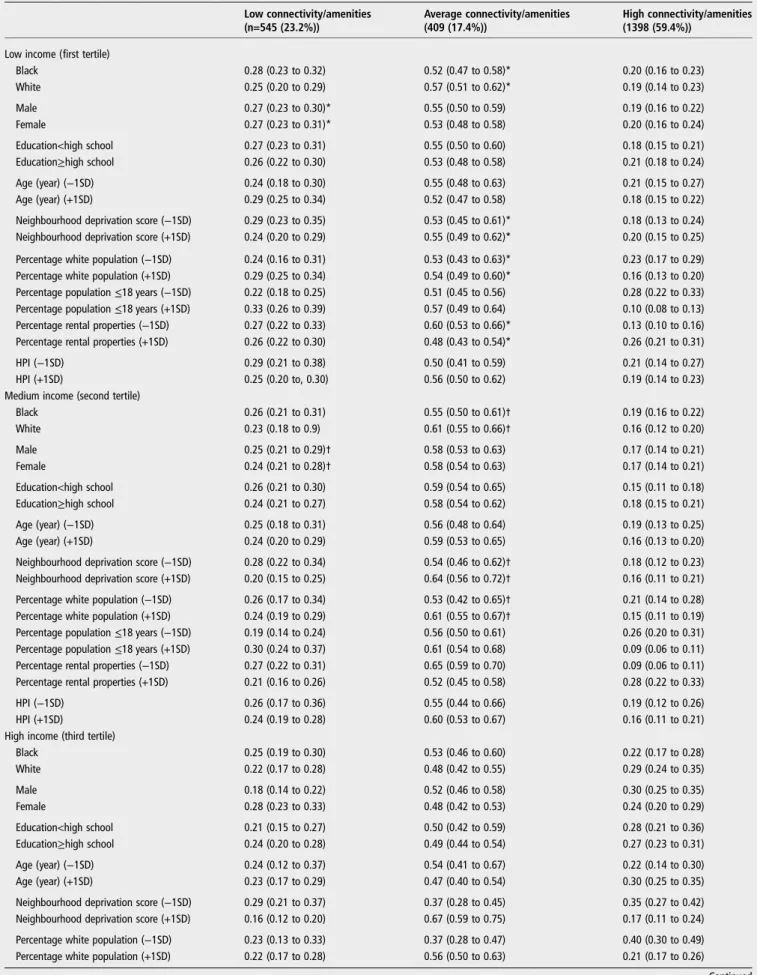
Table 3 Model-estimated‡multivariable-adjusted§ predicted probabilities (95% CI) of residing in low, average and high neighbourhood cluster types¶ by income status and levels (categories or ±1SD of mean) of covariates using multivariate multinomial logistic regression, CARDIA examination years 0–25
Low connectivity/amenities (n=545 (23.2%))
Average connectivity/amenities (409 (17.4%))
High connectivity/amenities (1398 (59.4%))
Low income (first tertile)
Black 0.28 (0.23 to 0.32) 0.52 (0.47 to 0.58)* 0.20 (0.16 to 0.23) White 0.25 (0.20 to 0.29) 0.57 (0.51 to 0.62)* 0.19 (0.14 to 0.23)
Male 0.27 (0.23 to 0.30)* 0.55 (0.50 to 0.59) 0.19 (0.16 to 0.22) Female 0.27 (0.23 to 0.31)* 0.53 (0.48 to 0.58) 0.20 (0.16 to 0.24)
Education<high school 0.27 (0.23 to 0.31) 0.55 (0.50 to 0.60) 0.18 (0.15 to 0.21) Education≥high school 0.26 (0.22 to 0.30) 0.53 (0.48 to 0.58) 0.21 (0.18 to 0.24)
Age (year) (−1SD) 0.24 (0.18 to 0.30) 0.55 (0.48 to 0.63) 0.21 (0.15 to 0.27) Age (year) (+1SD) 0.29 (0.25 to 0.34) 0.52 (0.47 to 0.58) 0.18 (0.15 to 0.22)
Neighbourhood deprivation score (−1SD) 0.29 (0.23 to 0.35) 0.53 (0.45 to 0.61)* 0.18 (0.13 to 0.24) Neighbourhood deprivation score (+1SD) 0.24 (0.20 to 0.29) 0.55 (0.49 to 0.62)* 0.20 (0.15 to 0.25)
Percentage white population (−1SD) 0.24 (0.16 to 0.31) 0.53 (0.43 to 0.63)* 0.23 (0.17 to 0.29) Percentage white population (+1SD) 0.29 (0.25 to 0.34) 0.54 (0.49 to 0.60)* 0.16 (0.13 to 0.20) Percentage population≤18 years (−1SD) 0.22 (0.18 to 0.25) 0.51 (0.45 to 0.56) 0.28 (0.22 to 0.33) Percentage population≤18 years (+1SD) 0.33 (0.26 to 0.39) 0.57 (0.49 to 0.64) 0.10 (0.08 to 0.13) Percentage rental properties (−1SD) 0.27 (0.22 to 0.33) 0.60 (0.53 to 0.66)* 0.13 (0.10 to 0.16) Percentage rental properties (+1SD) 0.26 (0.22 to 0.30) 0.48 (0.43 to 0.54)* 0.26 (0.21 to 0.31)
HPI (−1SD) 0.29 (0.21 to 0.38) 0.50 (0.41 to 0.59) 0.21 (0.14 to 0.27) HPI (+1SD) 0.25 (0.20 to, 0.30) 0.56 (0.50 to 0.62) 0.19 (0.14 to 0.23) Medium income (second tertile)
Black 0.26 (0.21 to 0.31) 0.55 (0.50 to 0.61)† 0.19 (0.16 to 0.22) White 0.23 (0.18 to 0.9) 0.61 (0.55 to 0.66)† 0.16 (0.12 to 0.20)
Male 0.25 (0.21 to 0.29)† 0.58 (0.53 to 0.63) 0.17 (0.14 to 0.21) Female 0.24 (0.21 to 0.28)† 0.58 (0.54 to 0.63) 0.17 (0.14 to 0.21)
Education<high school 0.26 (0.21 to 0.30) 0.59 (0.54 to 0.65) 0.15 (0.11 to 0.18) Education≥high school 0.24 (0.21 to 0.27) 0.58 (0.54 to 0.62) 0.18 (0.15 to 0.21)
Age (year) (−1SD) 0.25 (0.18 to 0.31) 0.56 (0.48 to 0.64) 0.19 (0.13 to 0.25) Age (year) (+1SD) 0.24 (0.20 to 0.29) 0.59 (0.53 to 0.65) 0.16 (0.13 to 0.20)
Neighbourhood deprivation score (−1SD) 0.28 (0.22 to 0.34) 0.54 (0.46 to 0.62)† 0.18 (0.12 to 0.23) Neighbourhood deprivation score (+1SD) 0.20 (0.15 to 0.25) 0.64 (0.56 to 0.72)† 0.16 (0.11 to 0.21)
Percentage white population (−1SD) 0.26 (0.17 to 0.34) 0.53 (0.42 to 0.65)† 0.21 (0.14 to 0.28) Percentage white population (+1SD) 0.24 (0.19 to 0.29) 0.61 (0.55 to 0.67)† 0.15 (0.11 to 0.19) Percentage population≤18 years (−1SD) 0.19 (0.14 to 0.24) 0.56 (0.50 to 0.61) 0.26 (0.20 to 0.31) Percentage population≤18 years (+1SD) 0.30 (0.24 to 0.37) 0.61 (0.54 to 0.68) 0.09 (0.06 to 0.11) Percentage rental properties (−1SD) 0.27 (0.22 to 0.31) 0.65 (0.59 to 0.70) 0.09 (0.06 to 0.11) Percentage rental properties (+1SD) 0.21 (0.16 to 0.26) 0.52 (0.45 to 0.58) 0.28 (0.22 to 0.33)
HPI (−1SD) 0.26 (0.17 to 0.36) 0.55 (0.44 to 0.66) 0.19 (0.12 to 0.26) HPI (+1SD) 0.24 (0.19 to 0.28) 0.60 (0.53 to 0.67) 0.16 (0.11 to 0.21) High income (third tertile)
Black 0.25 (0.19 to 0.30) 0.53 (0.46 to 0.60) 0.22 (0.17 to 0.28) White 0.22 (0.17 to 0.28) 0.48 (0.42 to 0.55) 0.29 (0.24 to 0.35)
Male 0.18 (0.14 to 0.22) 0.52 (0.46 to 0.58) 0.30 (0.25 to 0.35) Female 0.28 (0.23 to 0.33) 0.48 (0.42 to 0.53) 0.24 (0.20 to 0.29)
Education<high school 0.21 (0.15 to 0.27) 0.50 (0.42 to 0.59) 0.28 (0.21 to 0.36) Education≥high school 0.24 (0.20 to 0.28) 0.49 (0.44 to 0.54) 0.27 (0.23 to 0.31)
Age (year) (−1SD) 0.24 (0.12 to 0.37) 0.54 (0.41 to 0.67) 0.22 (0.14 to 0.30) Age (year) (+1SD) 0.23 (0.17 to 0.29) 0.47 (0.40 to 0.54) 0.30 (0.25 to 0.35)
Neighbourhood deprivation score (−1SD) 0.29 (0.21 to 0.37) 0.37 (0.28 to 0.45) 0.35 (0.27 to 0.42) Neighbourhood deprivation score (+1SD) 0.16 (0.12 to 0.20) 0.67 (0.59 to 0.75) 0.17 (0.11 to 0.24)
Percentage white population (−1SD) 0.23 (0.13 to 0.33) 0.37 (0.28 to 0.47) 0.40 (0.30 to 0.49) Percentage white population (+1SD) 0.22 (0.17 to 0.28) 0.56 (0.50 to 0.63) 0.21 (0.17 to 0.26)
to other urban areas. For example, the low amenities/connect-ivity neighbourhood type was characterised by greater land area and greater park size, which is consistent with previous work.29 The distribution of individuals across neighbourhood types also reflected the increasingly urban nature of neigh-bourhoods in the USA.30
Our study had several limitations, including a lack of data related to crime, school quality, car ownership or location of participants’actual (vs nearest) employment. We did not adjust for population density due to collinearity with our explanatory variables, and it is possible that much of neighbourhood selec-tion could have been predicted by urban versus suburban loca-tion. With the exception of food outlet business records, we could not evaluate the accuracy of our commercial data sets nor could we validate our clusters due to deductive disclosure. Finally, we did not know the extent to which participants were constrained to live in areas due to observed or unobserved factors (eg, discrimination); however, stratifying our models by individual-level income may have mitigated constraints related to affordability. With the exception of gender, it is also possible that associations between individual-level sociodemographics and neighbourhood characteristics with residential neighbourhood type differed by individual-level income level, but the magnitude of estimated effect may have been too small to detect in our sample.
Using time-varying data from the CARDIA study and four urban cities, we found that neighbourhood racial and age com-position and the percentage of rental properties were meaning-ful predictors of residential location type over time; but we did not observe similarfindings with individual-level race; age; and educational attainment, neighbourhood SES and housing prices. Ourfindings also showed that relationships between individual-level gender and residential neighbourhood type were stronger for high-income individuals. Overall, neighbourhood-level factors appeared to play a comparatively greater role in residen-tial location behaviour related to the food and built environ-ment than individual-level sociodemographics. Our study is an important first step in identifying how residential self-selection may bias estimates of the effects of the food and built environ-ment with health outcomes, and how this dynamic may differ across income levels.
What this study adds
▸ Being female was positively associated with living in neighbourhoods with low (vs high) road connectivity and activity-related and diet-related amenities among
high-income individuals, whereas individual-level race, age and education was not associated with residential location behaviour at any income level.
▸ Neighbourhood age and racial composition and the percentage of rental properties, but not neighbourhood socioeconomic status and housing prices, were associated with residential location behaviour related to the food and built environment at all income levels.
▸ Our study is an important step in understanding how residential location behaviour related to amenities and physical activity opportunities is influenced by
sociodemographic characteristics of the population, and may help mitigate residential self-selection bias in the food and built environment literature.
Acknowledgements The authors would like to acknowledge CARDIA chief reviewer Kiarri Kerhsaw, PhD, whose thoughtful suggestions improved the paper, as
Table 3 Continued
Low connectivity/amenities (n=545 (23.2%))
Average connectivity/amenities (409 (17.4%))
High connectivity/amenities (1398 (59.4%))
Percentage population≤18 years (−1SD) 0.14 (0.07 to 0.21) 0.48 (0.40 to 0.56) 0.38 (0.28 to 0.48) Percentage population≤18 years (+1SD) 0.33 (0.23 to 0.43) 0.53 (0.40 to 0.66) 0.14 (0.05 to 0.24) Percentage rental properties (−1SD) 0.25 (0.20 to 0.30) 0.61 (0.54 to 0.67) 0.14 (0.08 to 0.20) Percentage rental properties (+1SD) 0.10 (−0.001 to 0.21) 0.19 (0.04 to 0.34) 0.71 (0.50 to 0.91)
HPI (−1SD) 0.21 (0.10 to 0.33) 0.41 (0.29 to 0.53) 0.38 (0.26 to 0.50) HPI (+1SD) 0.23 (0.18 to 0.27) 0.48 (0.43 to 0.53) 0.29 (0.25 to 0.34)
Referent outcome=high road connectivity and activity-related and diet-related amenities.
*Indicates that the difference in the predicted probabilities in the low income tertile are statistically significantly different than the difference in the predicted probabilities in the high income tertile within each neighborhood cluster type, at the p<0.05 level.
†Indicates that the difference in the predicted probabilities in the medium income tertile are statistically significantly different than the difference in the predicted probabilities in the high income tertile within each neighborhood cluster type, at the p<0.05 level.
‡Predicted probabilities were generated from the model coefficients and depict the probability of residing in neighbourhoods with low (vs high) road connectivity and activity-related and diet-related amenities at fixed levels of the covariates (categories or ±1SD of mean).
§Variables include individual-level race, gender, educational attainment and age; neighbourhood-level deprivation score, percentage white population, percentage population≤18 years and HPI; examination year (time); and baseline study centre.
¶Neighbourhood clusters created using non-hierarchical cluster analysis of measures related to connectivity and neighbourhood amenities, including intersection density (number of three-way, four-way and higher intersections per km2), links (count), cul-de-sacs (count),β-index (ratio of links to nodes), total road length (km), percentage residential (of total road
length, km), distance from participants’residential location to nearest employment centre centroid (km), total park area within each neighbourhood (km2), and total physical activity
facilities, supermarkets, co-ops and chain fast food restaurants (separately; count per km2land).
CARDIA, Coronary Artery Risk Development in Young Adults; HPI, housing price index.
What is already known on this subject
▸ Understanding the influence of the food environment and physical activity amenities on residential location behaviour is essential for addressing residential self-selection bias. ▸ However, not much is known about how the food and built
environment influences residential location behaviour, and how associations may differ by income status.
well as Marc Peterson, of the University of North Carolina, Carolina Population Center (CPC) and the CPC Spatial Analysis Unit for creation of the environmental variables. PER, MPH had full access to all of the data in the study and takes responsibility for the integrity of the data and the accuracy of data analysis. Contributors PER had full access to the data and takes responsibility for the integrity of the data and the accuracy of the data analysis. PER performed the statistical analysis, and analysed and interpreted the data. PER and PG-L drafted the article. DKG, JMS, JPR and PG-L critically revised the article for important intellectual content. PG-L acquired the data, obtained the funding, approved thefinal draft of the article and supervised the study. All authors contributed to the study concept and design.
Funding This work was funded by the National Heart, Lung, and Blood Institute (NHLBI) R01HL104580. The Coronary Artery Risk Development in Young Adults Study (CARDIA) is supported by contracts HHSN268201300025C,
HHSN268201300026C, HHSN268201300027C, HHSN268201300028C, HHSN268201300029C and HHSN268200900041C from the NHLBI, the Intramural Research Program of the National Institute on Aging (NIA), and an intra-agency agreement between NIA and NHLBI (AG0005). The authors are grateful to the Carolina Population Center, University of North Carolina at Chapel Hill, for general support (grant P2C HD050924 from the Eunice Kennedy Shriver National Institute of Child Health and Human Development (NICHD)), the Nutrition Obesity Research Center (NORC), University of North Carolina (grant P30DK56350 from the National Institute for Diabetes and Digestive and Kidney Diseases (NIDDK)), and to the Center for Environmental Health Sciences (CEHS), University of North Carolina (grant P30ES010126 from the National Institute for Environmental Health Sciences (NIEHS)).
Competing interests None declared.
Provenance and peer reviewNot commissioned; externally peer reviewed. Open Access This is an Open Access article distributed in accordance with the Creative Commons Attribution Non Commercial (CC BY-NC 4.0) license, which permits others to distribute, remix, adapt, build upon this work non-commercially, and license their derivative works on different terms, provided the original work is properly cited and the use is non-commercial. See: http://creativecommons.org/ licenses/by-nc/4.0/
REFERENCES
1 Boone-Heinonen J, Gordon-Larsen P, Guilkey DK,et al. Environment and physical activity dynamics: the role of residential self-selection.Psychol Sport Exerc 2011;12:54–60.
2 Kim JH, Pagliara F, Preston J. The intention to move and residential location choice behaviour.Urban Stud2005;42:1621–36.
3 Pinjari AR, Bhat CR, Hensher DA. Residential self-selection effects in an activity time-use behavior model.Transportation Res Part B Methodol2009;43:729–48. 4 Pinjari AR, Pendyala RM, Bhat CR,et al. Modeling the choice continuum: an
integrated model of residential location, auto ownership, bicycle ownership, and commute tour mode choice decisions.Transportation2011;38:933–58. 5 Bhat CR, Guo JY. A comprehensive analysis of built environment characteristics on
household residential choice and auto ownership levels.Transportation Res Part B Methodol2007;41:506–26.
6 Smith B, Olaru D. Lifecycle stages and residential location choice in the presence of latent preference heterogeneity.Environ Plann A2013;45:2495–514.
7 Sugiyama T, Neuhaus M, Cole R,et al. Destination and route attributes associated with adults’walking: a review.Med Sci Sports Exerc2012;44:1275–86. 8 Cho EJ, Rodriguez D, Song Y. The role of employment subcenters in residential
location decisions.J Transport Land Use2008;1:21–51.
9 Chen C, Gong H, Paaswell R. Role of the built environment on mode choice decisions: additional evidence on the impact of density.Transportation 2008;35:285–99.
10 Habib MA, Miller EJ. Reference-dependent residential location choice model within a relocation context.Transportation Res Rec2009;2133:92–9.
11 Zondag B, Pieters M. Influence of accessibility on residential location choice. Transportation Res Rec2005;1902:63–70.
12 Schirmer PM, van Eggermond MA, Axhausen KW. The role of location in residential location choice models: a review of literature.J Transport Land Use2014;7:3–21. 13 Lewis PG, Baldassare M. The complexity of public attitudes toward compact
development: survey evidence fromfive states.J Am Plann Assoc2010;76:219–37. 14 Liao FH, Farber S, Ewing R. Compact development and preference heterogeneity in
residential location choice behaviour: a latent class analysis.Urban Stud 2015;52:314–37.
15 Zillow Neighborhood Boundaries. http://www.zillow.com/howto/api/ neighborhood-boundaries.htm (access Date: 5/15/2015).
16 Hirsch JA, Meyer KA, Peterson M,et al. Obtaining longitudinal built environment data retrospectively across 25 years in four US cities.Front Public Health2016;4:65. 17 Cao X, Handy SL, Mokhtarian PL. The influences of the built environment and
residential self-selection on pedestrian behavior: evidence from Austin, TX. Transportation2006;33:1–20.
18 Walker RE, Keane CR, Burke JG. Disparities and access to healthy food in the United States: a review of food deserts literature.Health Place2010;16:876–84. 19 Hammer J, Howell S, Bytzer P,et al. Symptom clustering in subjects with and
without diabetes mellitus: a population-based study of 15,000 Australian adults. Am J Gastroenterol2003;98:391–8.
20 Messer LC, Laraia BA, Kaufman JS,et al. The development of a standardized neighborhood deprivation index.J Urban Health2006;83:1041–62. 21 Chen C, Burgos AC, Mehra S,et al. The Moody’s analytics Case-Shiller® home
price index forecast methodology.Moodys Anal2011. http://www.moodysanalytics. com/~/media/Brochures/Economic-Consumer-Credit-Analytics/Examples/case-shiller-methodology.pdf (accessed online Aug 2016).
22 Cao XJ. Disentangling the influence of neighborhood type and self-selection on driving behavior: an application of sample selection model.Transportation 2009;36:207–22.
23 Prashker J, Shiftan Y, Hershkovitch-Sarusi P. Residential choice location, gender and the commute trip to work in Tel Aviv.J Transport Geography 2008;16:332–41.
24 Friedman S, Rosenbaum E. Does suburban residence mean better neighborhood conditions for all households? Assessing the influence of nativity status and race/ ethnicity.Soc Sci Res2007;36:1–27.
25 Mokhtarian PL, Cao X. Examining the impacts of residential self-selection on travel behavior: a focus on methodologies.Transportation Res Part B Methodol 2008;42:204–28.
26 Vyvere Y, Oppewal H, Timmermans H. The validity of hierarchical information integration choice experiments to model residential preference and choice. Geographical Anal1998;30:254–72.
27 Bhat CR, Guo J. A mixed spatially correlated logit model: formulation and application to residential choice modeling.Transportation Res Part B Methodol 2004;38:147–68.
28 Bruch EE, Mare RD. Methodological issues in the analysis of residential preferences, residential mobility, and neighborhood change.Sociol Methodol 2012;42:103–54.
29 Abercrombie LC, Sallis JF, Conway TL,et al. Income and racial disparities in access to public parks and private recreation facilities.Am J Prev Med 2008;34:9–15.