Statistical Analysis on Market Microstructure
Models
by Feng Liu
A Dissertation submitted to the faculty of the University of North Carolina at Chapel Hill in partial fulfillment of the requirements for the degree of Doctor of Philosophy in the Department of Statistics and Operation Research.
Chapel Hill 2010
Approved by:
Chuanshu Ji, Advisor
c
2010 Feng Liu
Abstract
FENG LIU: Statistical Analysis on Market Microstructure Models (Under the direction of Chuanshu Ji.)
Acknowledgments
I am largely indebted to Prof. Chuanshu Ji, who has been such a great advisor and mentor to me. His ingenious ideas and deep insight have constantly inspired me and guided me through the past five years. And his knowledge of statistics and financial mathematics has been a great source of enlightenment to me. I am especially gratefully for his great effort on my research topics and process.
My sincere gratitude also goes to other members of my committee. Prof. G¨unter Strobl from finance has been a great mentor to me and provides enormous support of my research. He has not only instructed me on microstructure topics but also interpreted the intricacy of microstructure issues with patience especially as I am coming from statistics major. His profound knowledge and valuable advices enlighten me throughout my research. Prof. Douglas Kelly, Prof. Nilay Argon and Prof. Shankar Bhamidi have read my dissertation carefully and provided numerous useful comments and feedbacks. I also learned a lot from the interesting courses they taught.
Table of Contents
Abstract iii
List of Figures viii
List of Tables x
1 Introduction 1
2 Basic Formulation and Major Topics 8
2.1 Overview . . . 8
2.2 Market dynamics . . . 9
2.2.1 Price movement and information set . . . 9
2.2.2 Issues and interpretation . . . 11
2.3 Generalized Roll model . . . 12
2.3.1 Roll model . . . 12
2.3.2 Hasbrouck’s approach . . . 14
2.4 Sequential trade model . . . 15
2.5 Strategic trade model . . . 18
3 Data Structure and Empirical Study 22 3.1 Trade volume or order imbalance . . . 22
3.3 Asymmetric information . . . 26
3.4 Market depth . . . 28
3.5 Market liquidity . . . 30
4 Liquidity in market microstructure models 31 4.1 Liquidity and expect returns . . . 31
4.2 Liquidity measures . . . 32
4.2.1 Bid-ask spread . . . 34
4.2.2 Kyle’s λ . . . 35
4.2.3 Daily returns, trading volume and ILLIQ . . . 37
4.3 Liquidity risk . . . 38
5 Inference on an Extended Kyle’s Model 40 5.1 New derivation of Kyle’s equilibrium solution . . . 41
5.1.1 The original derivation of Kyle’s solution . . . 44
5.1.2 An alternative characterization of Kyle’s solution . . . 45
5.2 An extension of Kyle’s model . . . 50
5.2.1 The single period case . . . 50
5.2.2 The multiple period case . . . 53
5.3 Simulation study of Kyle’s equilibrium solution . . . 55
6 Dynamic Bayesian Inference 60 6.1 Basic notions . . . 61
6.2 Time series in Bayesian framework . . . 62
6.3 Dynamic Bayesian Model . . . 64
6.4 The Model . . . 66
6.5 Markov Chain Monte Carlo (MCMC) . . . 69
6.5.2 MCMC for original Kyle’s model . . . 72
6.5.3 MCMC for our dynamic Bayesian model . . . 74
6.6 Simulation . . . 77
7 Empirical studies and Bayesian model selection 85 7.1 Data . . . 85
7.2 Dynamic Model vs. original Kyle’s Model . . . 86
7.3 Model fitting with different sample periods . . . 91
7.4 Sample stocks . . . 93
7.5 Bayesian model selection . . . 98
8 Other Topics 102
9 Conclusions 110
List of Figures
2.1 Sample Cisco trade price, bid, ask quotes . . . 9
3.1 Relationship between trade volume and return . . . 22
3.2 MSFT intraday bid-ask spread movement . . . 26
3.3 MSFT trade price movement . . . 27
3.4 Aggregated intraday order imbalance vs. price change . . . 28
3.5 Line fit with market depth (or λn) . . . 29
4.1 Relationship between stocks’ excess monthly returns and bid-ask spreads 35 5.1 {dn} series with various sample periods N . . . 48
5.2 {βn} and {λn} series with various sample periods N . . . 49
5.3 Kyle model parameters, β, λ, α, δ,Σ . . . 57
5.4 Order flows, trade prices and profit . . . 58
6.1 Insiders’ strategy, original vs. MCMC for our model . . . 78
6.2 Reciprocal of market depth, original vs. MCMC for our model . . . 79
6.3 Bayesian results of order flows . . . 81
6.4 Parameter and deviance trace plots . . . 81
6.5 Parameter and deviance density estimates . . . 82
6.6 Parameter and deviance autocorrelation plots . . . 83
6.7 MCMC Estimates of beta via original Kyle’s model vs. actual beta . . 84
7.1 Insiders’ strategy, MCMC for dynamic model on IBM 2008Q3 . . . 87
7.2 Trade prices on IBM prior to 2008Q3 earning announcement . . . 88
7.4 Reciprocal of market depth, MCMC for our model on IBM 2005Q2 . . 89
7.5 Beta, MCMC for original Kyle’s model on IBM 2008Q3 . . . 90
7.6 Lambda, MCMC for original Kyle’s model on IBM 2008Q3 . . . 90
7.7 MCMC for dynamic model using different length of data . . . 92
7.8 MCMC for original Kyle’s model using different length of data . . . 92
7.9 Results of IBM through four different periods . . . 93
7.10 Results of BA through four different periods . . . 94
7.11 Results of FUN through four different periods . . . 95
7.12 Results of LUK through four different periods . . . 96
List of Tables
3.1 Summary statistics of daily returns vs. daily volume . . . 23 3.2 Sample first-order autocorrelation of trade direction . . . 25
6.1 Parameters and Deviance Bayesian results . . . 80 6.2 Parameters and Deviance Bayesian results via original Kyle’s model . . 84
Chapter 1
Introduction
The need for studies in financial economics becomes more urgent than ever after we have experienced the recent downturns in financial markets. Statistics play an increasing role in such studies. In the literature of mathematical finance and related statistical analysis, most of the elegant results hold under the assumption of a “perfect market” or “fully efficient market”, i.e. no transaction costs, no bid/ask spread, same information shared by all market participants, no tax, no limit for short selling, etc. Conceivably that is far from what happens in real financial markets. The area of market microstructure studies what factors and mechanisms affect an asset price, how informed traders and uninformed ones differ in obtaining information and using it to optimize their trading strategies, etc. Research in this area ultimately will enhance our understanding of the real markets and have more practical impacts on various issues. That is what we plan to study.
are the investors who demand or supply the ultimate immediacy and the dealers who facilitate the trading. An investor usually wishes to trade immediately and to buy low and sell high. In reality however, traders actually buy at an (higher) ask price and sell at a (lower) bid price. Those bid/ask prices are quoted by dealers (market makers, limit order traders), and the spread “ask price minus bid price” is the compensation that dealers receive for offering immediacy.
The literature on asset pricing often assumes that markets operate without costs and frictions whereas the essence of the market microstructure research is to analyze the impact of trading costs and various friction factors. The investors are generally involved in the market for securities and related information. The market for securities deals with the determinants of security prices such as earning per share etc. The market for information deals with the supply and demand of information. It incorporates the incentives of security analysis and related information transfer. The asymmetric information is closely related to transaction services since the cost of a trade depends on the information possessed by the participants in the trade.
Market microstructure studies market friction and asymmetric information impact on security prices. When we look at the security price dynamics with respect to market microstructure, our focus has shifted from monthly or daily to minute or tick level with more features such as bid price, ask price, bid size, ask size, trade price and trade volume etc. The additional features of price and trading dynamics reflect the complexity of microstructure.
Let Ft be the information set available to the market at time t, the payoff of a
security be a random variable, denote by v. Then the conditional expectation pt =
E(v|Ft) is referred to as the fundamental value or the efficient price of the security.
The information set is the starting point for many microstructure models. One of the basic goals of microstructure analysis is a detailed study of how informational efficiency arises, and the process by which new information comes into play or is reflected in the price movement. In microstructure analysis, transaction prices are usually not martingales. By imposing economic or statistical structure, it is often possible to identify a martingale component of the price with respect to a particular information set.
The public information set consists of some common knowledge concerning a proxy of probability structure of the economy, i.e. various possible scenarios of a terminal security value and associated types of agents. Most models make no provision for the updates of non-trade public information (e.g., news release). As trading unfolds, the most important updates to the public information set are market data, such as bid, ask, closing prices and volumes of trades. Private information may consist of signals about security value, i.e. more detailed knowledge of the terminal security value.
When all agents areex anteidentical, they are said to be symmetric. This does not exclude private values or private information. The symmetry means that all individual-specific variables (e.g., the coefficient of risk aversion, the signal) are identically dis-tributed across all agents. The Roll model is still informational symmetric. In an
asymmetric information model, a subset of agents has superior private information which leads to a trading advantage.
The majority of asymmetric information models in market microstructure examines market dynamics subject to a single source of uncertainty. At the end of the trading, the security payoff is known and realized. Thus, the trading process is an adjustment from one well-defined information set to another set. The dynamics are neither stationary nor ergodic, although path realizations could be stacked to disclose trading behaviors. There are two main sorts of asymmetric models, among others:
(a) Sequential trade model
Randomly selected traders arrive at the market one by one, sequentially, and
is profitable, they trade as much as possible.
(b) Strategic trade model
A seminal strategic model is studied in Kyle (1985). The Kyle model is a model of a batch-auction market, in which market makers see the order imbalance at each auction date. And market makers compete to fill the order imbalance, and matching orders are executed at market clearing prices. Unlike the sequential trade model, the strategic informed agent could trade at multiple times. Kyle develops the optimal trading behavior for the informed trader and shows that the agent will trade on his information only gradually, rather than exploit it to the maximum extent possible.
The essence of both models is that a trade from the informed trader will reveal his/her private information assuming traders are all rational. The ”buy” order orig-inates from a trader who has positive private information, but not from those who possess negative information (here we rule out ”bluffing”, i.e. the informed trader is ”bluffing” if he knowingly sells an undervalued or buys an overvalued asset). And the competitive market makers will set their bid-ask quotes accordingly. In consequence, greater information asymmetry would lead to wider spreads in quotes. The spread and trade impact are major empirical implications of these models.
There is an extensive literature in market microstructure. Besides many research and survey papers, here we mention several good books: Brunnermeier (2001), de Jong, F. and Rindi, B. (2009), Harris, L. (2003), O’Hara, M. (1995), and Vives, X. (2008).
resulting constrained optimization problem is tackled, and its equilibrium solution will yield an optimal trading strategy from the perspective of each market participant, and a risk-neutral clearing price for every traded asset. In particular, the solution often enables us to interpret the economic impacts of certain parameters contained in the model. On the statistical side, inference on model parameters is performed based on real market data, usually represented by time series of asset prices and returns, trading volumes, orders and quotes, etc. whether they are daily or involving intra-day activities. More often than not, goodness-of-fit of the proposed model need not be satisfactory. Naturally, more sophisticated models can be considered. However, a purely statistical approach based on goodness-of-fit may not address the issue of economic interpretation. Financial economists always pay greater attentions to what we can learn from a model. To reconcile the economic and statistical aspects, a natural “spiral up” development can start with a basic economic model, fit it by market data; With observed deviations between the data and the proposed model, we proceed to modify the model and try to derive the corresponding equilibrium solution, then check it with data again, etc. The hope is to improve the goodness-of-fit and enhance the understanding of market behaviors in each new iteration along such a research path.
This approach will be illustrated in a framework of the celebrated strategic trade model in Kyle (1985). We aim at fitting several extensions of Kyle’s models using intra-day data, and retaining its interpretability. Dynamic Bayesian modeling [see West and Harrison (1997)] appears to fit our need, because in many problems sequential updating between observed data and various unknowns follow a natural path. The unknowns include model parameters (e.g. market depth and noise trading volatility) and latent variables (e.g. an inside trader’s order).
solutions. The algorithm we provide offers a computationally more efficient way to char-acterize the equilibrium solutions, which also enables us to develop similar equilibrium solutions in certain extensions to Kyle’s model, such as the one with noisy signals of the asset value observed by the informed trader. We also propose an extended model to Kyle’s in which the (reciprocal of) market depth{λn} and the informed trading
in-tensity {βn} form time series. A Bayesian inference procedure based on real intra-day
Chapter 2
Basic Formulation and Major
Topics
2.1
Overview
2.2
Market dynamics
2.2.1
Price movement and information set
When we look at the security price dynamics with respect to microstructure, our focus has shifted from monthly or daily to minute or tick level with more features at fine granularity. Such features include bid price, ask price, bid size, ask size, trade price and trade volume etc. The following figure illustrates ticker CSCO (Cisco System) traded on Jan, 3 2002 at second level, data source from TAQ (Trade and Quote) database. The trade price is augmented by bid/ask price quotes.
Figure 2.1: Sample Cisco trade price, bid, ask quotes
The three prices (bid, ask, and trade) differ. The ask (solid) is always higher than the bid (dot-dashed), and trades (dashed) usually occurs at posted bid and ask prices, but not always. They converge to each other. Those features reflect the complexity of market microstructure.
regular point of time. The random-walk model with drift is: For t= 1,2, ...,
pt = pt−1 +µ+ut, (2.1)
where ut are iid N(0, σ2) random variables, and µ is the expected price change (the
drift). In microstructure data samples the mean of µ is often small relative to its estimation variance, i.e,E(µ)< V ar(µ). It is often preferable to drop the mean return from the model in most microstructure analysis.
When µ= 0, E(pt|pt−1, pt−2, ..) =pt−1, where E(|pt|)<∞for all t. The pt process
follows a martingale. A more general definition involves conditioning on information sets.
Let Ft be the information set available to the market at the time t, the payoff
of a security is a random variable, denote as v. Then the conditional expectation pt=E(v|Ft), for all t is a martingale with respect to sequence of information sets Ft.
When the conditional information is all public information, the conditional expectation is referred to as the fundamental value of the security.
In microstructure analysis, transaction prices are usually not martingales. By im-posing economic or statistical structure, it is often possible to identify a martingale component of the price with respect to a particular information set. In the random-walk equation (2.1), ut are iid, the price process are time-homogeneous, that is, it
valid choice to describe market behavior in the long-run.
2.2.2
Issues and interpretation
In equation (2.1), price change is ∆pt = pt−pt−1, which is iid with mean 0, variance
V ar(ut) =σ2, andµset to 0. When we analyze the actual data samples, the short-run
security price changes always exhibits extreme dispersion and auto-correlation between successive observations.
For financial security data samples, the price changes at time horizon often have sample distributions with fat tails. The standard assumption that price changes are normally distributed is violated. For a random variable X, the population moment of orderαis defined asEXα. IfEXα is finite, asx→ ∞, then the corresponding sample estimate P
Xtα/T,T is the sample size, is the consistent estimate of of EXα. To get a consistent estimate of the standard error of mean, we require a consistent estimate of the variance. Not all moments are finite if the normal assumption is violated. Recent studies suggest that finite moments for daily equity returns exist only up to order 3, and the trading volume only up to order 1.5 (Gabaix 2003). These findings impose substantial restrictions on the sort of microstructure models we could estimate. The existence of extreme values in finite samples may lead to many practical consequence. Increasing the sample size may not increase the precision as fast as we expected, and estimated parameters are very sensitive to model specification.
The price increments ∆pt in the random walk are iid and uncorrelated. But data
samples show the first-order autocorrelations of price changes are usually negative and non-zero. For time series ∆pt, the autocovariance and autocorrelation is defined as
γk = Cov(∆pt,∆pt−k) and ρk = Corr(∆pt,∆pt−k). When the mean is zero, γk could
be estimated as the sample average ˆγk=T−1
PT
t=1∆pt∆pt−k, and the autocorrelations
We collect the data from WRDS TAQ database. The data samples we studied are MSFT (microsoft Inc) trade prices from Jan, 2 to Jan, 5 2002. There are 200,000+ trades in MSFT at tick level. The estimated first-order autocorrelation of price incre-ments is ˆρ1 =−0.4561, with standard error of 0.004. The p-value of significance test is
less than 10−5 which rejects zero autocorrelation hypothesis.
We would expect to find ˆρk = 0 for k = 1 for a random walk model. But the
empirical study verifies the contrary. The economic explanation about this contradic-tion motivates the Roll model, which explains autocorrelacontradic-tions of price increments by meaningful economic and statistic implication.
2.3
Generalized Roll model
2.3.1
Roll model
Roll (1984) suggests a model of high frequency trade prices which incorporate market dynamics. This model is fundamental to many market microstructure models such that it illustrates the distinction between price movement due to fundamental security value and those attribute to market organization and trading mechanism. The former arises from the earning capability and future cash flows of the underlying security, whereas the later are transient due to market behavior. The model provides meaningful economic interpretation, and in some cases, explains the market movement well.
For t= 1,2, ...,
pt = mt+c qt, (2.2)
mt = mt−1+ut, (2.3)
wheremtdenote the martingale efficient price at tth trade,ptis the trade price. Theqt
are direction indictors, which take on the value 1 (buy) or -1 (sell) with equal probability, the shocksu1, u2, ...are iid N(0, σ2) random variables, the parameters c >0 andσ >0
represent the effective cost and the volatility respectively. The two sequences{qt} and
{ut}are assumed to be independent. Note that only{pt}are observed, while{mt}and
{qt} are treated as latent variables.
The model implies
∆pt = c∆qt+ut, (2.4)
from which it follows that c = [−cov(∆pt,∆pt−1)]1/2, if cov(∆pt,∆pt−1) < 0, and
c = 0, otherwise. The first-order autocovariance is non-zero. ∆pt exhibits volatility
and negative serial correlation as the result of effective cost. The intuition is: If mt is
fixed so that prices take on only two values, the bid and the ask, and if the current price is the ask, then the price change between the current price and the previous price must be either 0 or −2c, and the price change between the next price and the current price must be either 0 or 2c. The moment estimate is feasible, however, only if the first-order sample autocovariance of the price change is negative.
If the dealers compete to the point where the costs are just covered, the bid and the ask aremt−candmt+c, with the spread 2c, a constant. We collect the data of 200,000
trades for MSFT on Jan, 2 to Jan, 5 2002 from TAQ, the first-order autocovariance is ˆ
γ1 = −0.00522. This implies c= $0.035, and bid-ask spread of 2c= $0.070; while the
2.3.2
Hasbrouck’s approach
To estimate the effective trading cost and returns formed from daily data, Hasbrouck advocates a Bayesian approach based on the Roll model. This method accommodates a long time span by daily data, and the cost estimate is validated against microstructure data.
The unknowns comprise both the model parameters{c, σ2}and the latent data{qt}.
We could get posterior distribution f(c|σ2, p
1, p2, ..., pT) and f(σ2|c, p1, p2, ...pT) via
multivariate Bayesian methods. However, the posterior joint densityf(c, σ2|p
1, p2, ..., pT)
is not obtained in a closed-form. This motivates the Gibbs sampler. The Gibbs sam-pler constructs full posterior densities by iteratively simulating from full conditional distributions forc, σ and qt.
The trading cost estimates from US stocks are formed from daily CRSP data. The CRSP/Gibbs estimates are very close to TAQ estimates (with correlation 0.96), which shows that the daily Gibbs estimates have strong validity. The estimation procedure tries to resolve the two components among the sample price path: the permanent innovations (due to the efficient price), and the transient effective cost (due to bid-ask effect). Whenc >> σ, the bid/ask bounce generates reversals that are easy to pick out which leads to clear resolution of the two components. When c is relative small, the bid/ask effect is swamped by innovations in the efficient price.
Empirical sample results:
• Ticker symbol NEWE (Jan 1990) bid = 3.625, ask = 4.125, c ≈ 0.25, daily volatility σ= 0.031 clear resolution
• Ticker symbol MSFT (Jan 2005) bid= 26.67, ask= 26.68, c≈0.005, σ = 0.073 poor resolution
price, it nevertheless lacks completeness in terms of determinants. For expected returns, it shows weak evidence of trading cost as a characteristic, and it shows no evidence that the trading cost variation is a risk factor. In fact, Glosten and Milgrom (1985) argues that c is determined endogenously and is unlikely to be independent of {mt},
the permanent component.
Most microstructure models including Roll model are dynamic over time and have latent variables. Dynamic latent variable models can be formulated in state-space form and estimated by maximum likelihood. For Gaussian cases, it could be estimated using multivariate linear regression; For non-Gaussian latent variables(e.g., the buy/sell indicator), the estimation procedure often involves nonlinear smoothing or Bayesian MCMC methods. Hasbrouck’s work sheds light on Bayesian type of analysis.
2.4
Sequential trade model
We begin with Glosten-Milgrom model. Consider one security valued at V ∈ {Vh, Vl},
with Pr(Vl) = δ. The value is revealed at the end of trade. There are two types of
traders: the informed I and the uninformed U, the proportion of informed traders among the population is µ. The market maker posts bid and ask quotes,B and A. A trader is randomly drawn from the population. If the trader is informed, he buys if V = Vh, sells if V = Vl. If the trader is uninformed, she buys or sells randomly with
equal probability. The market maker does not know the types of the trader. A buy is a purchase by the trader at the dealer’s ask price, A; a sell is a trading at the bid, B. We assume that the competition among dealers drives the expected profit to zero. The market maker’s inference given that the first trade is a buy or a sell can be summarized by his posterior belief about the low outcome.
Let pk(buy), (orpk(sell)) k = 1,2..., denote the probability of a low outcome given
outcome, which isδ. Let Bk denotekth order is buy,Sk denote kthorder is sell. Then
the market maker’s posterior belief of a low outcome after the first trade is buy is,
p1(buy) = Pr(Vl|B1) =
Pr(Vl, buy)
Pr(buy) =
δ(1−µ)
1 +µ(1−2δ), (2.5)
and dealer’s expectation of the value given first buy order isE(V|B1) = Pr(Vl|buy)Vl+
(1−Pr(Vl|buy))Vh. If competition drives the expected profit to zero, then the posted
”ask price” is the dealer’s expected value.
A=E(V|B1) =
δ(1−µ)Vl+ (1−δ)(1 +µ)Vh
1−(1−2δ)µ , (2.6)
The bid price is similar, followed by a sell to the dealer. The dealer saw the first trader is a sell order and post the bid price.
p1(sell) = Pr(Vl|S1) =
Pr(Vl, sell)
Pr(sell) =
δ(1 +µ)
1−µ(1−2δ), (2.7) B =E(V|S1) =
δ(1 +µ)Vl+ (1−δ)(1−µ)Vh
1 + (1−2δ)µ , (2.8)
The bid-ask spread is:
S =A−B = 4(1−δ)δ(Vh−Vl)µ
1−(1−2δ)2µ2 , (2.9)
The dealer updates his belief and posts new quotes on each trades sequentially. This process repeats for k=1,2,... This updating procedure could be expressed in general forms since all probabilities in the event tree are constant exceptpk(.).
pk(buy|pk−1(.)) =
pk−1(.) (1−µ)
1 +µ(1−2pk−1(.))
, (2.10)
pk(sell|pk−1(.)) =
pk−1(.) (1 +µ)
1−µ(1−2pk−1(.))
It can be shown that pk(buy|pk−1(buy), pk−2(sell)) = pk(buy|pk−1(sell), pk−2(buy)), for
all k. The arrival sequence of the buy or sell orders does not matter. Therefore the proportion of buy or sell orders is deterministic to the outcome.
The conditional expectation of the ask can be decomposed as
A=E(V|buy) = E(V|U, buy) Pr(U|buy) +E(V|I, buy) Pr(I|buy), (2.12)
rearranging terms gives
(A−E(V|U, buy)) Pr(U|buy) = −(A−E(V|I, buy)) Pr(I|buy), (2.13)
In this model, the economic interpretation for equation (2.13) is that the gain from an uninformed trader on the left side is equal to the loss to the informed trader on the right side (subject to zero profit expectation for the market maker). There is net wealth transfer from the uninformed to the informed.
Although the trader is independently drawn from both population for order execu-tion, one subset of the population (the informed) always trade in the same direction. The result is that orders are serially correlated. We will do empirical study on this topic in the next chapter.
One important economic justification of G-M model is trades update the price. For any security at kth given trade, a buy order on the (k+ 1)th trade will make a upward revision in the conditional probability of a high outcome, and consequently increase both ask and bid quotes and drive trading price upward. In contrast, a sell order will drive price downward. The trade price impact is a particular useful empirical implication.
In the Roll model, we denote {qt} as the trade direction variable (+1 buy, -1 sell)
attributes to asymmetric information processed by difference traders, the informed traders always trade in the direction of his knowledge.
The asymmetric information in the G-M model isµ, the proportion of the informed trader in the population. In equation (2.11) and (2.9), the asymmetric information parameterµis positively related topk(sell), and the bid-asked spread. The justification
behind is when the market have more informed traders, a sell order will be more likely submitted by an informed trader instead of a uninformed, the probability of a low outcome after sell is high; similarly, the probability of a high outcome given buy order is also high. In consequence, the dealer will post wider bid-ask spread in response to the change of posterior beliefs. These results suggest use of the bid-ask spread or the impact of an order has on subsequent prices as proxies for the asymmetric information. We have more discussions in the empirical study.
The limitation of G-M model is the informed traders are drawn randomly by the market mechanism. When she is selected, she will trade once and the maximum (one unit of order). There are no trading strategies for the informed trader to maximize her profit. The order execution timing and order sizes are two important aspects to the informed in empirical work while remain unaddressed in G-M model.
2.5
Strategic trade model
We follow the basic framework in Kyle (1985) with modified notation.
• Fix an asset in what follows. Suppose N auctions take place sequentially over a trading period (e.g. day, month, year). For each n = 0,1, . . . , N, tn denotes the
time for the nth auction, with 0 =t0 < t1 <· · ·< tN = 1.
so that ∆Xn =Xn−Xn−1 denotes the quantity traded by the insider at the nth
auction. However, V ∼ N(p0,Σ0) is considered as a random variable by a set of
noise traders.
• The quantity traded by noise traders at the nth auction is denoted by ∆Un ∼
N(0, σ2∆t
n) with ∆tn =tn−tn−1. Assume U1, ..., UN are independent, and V is
independent of{U1, ..., UN}.
• Letpn be the asset’s market clearing price at the nth auction, ∆Yn = ∆Xn+ ∆Un
denote the total orders at the nth auction. The information set FU
n available to
uninformed traders (including a market maker and all noise traders) attnconsists
of the observations{p1, ..., pn; ∆Y1, ...,∆Yn}.
• The informed trader (insider) has a richer information set available to him before making his move at the nth auction. Such a set FI
n−1 includes {X1, ..., Xn−1;V}
in addition to FU
n−1. The insider chooses ∆Xn based on FnI−1.
• After the move made by both insider and noise traders at the nth auction, the market maker determines the price pn based on FnU−1 and ∆Yn.
•Let
πn= N
X
i=n
(V −pi) ∆Xi (2.14)
be the total profits of the insider to be made at auctions n, n+ 1, ..., N, and X = (X1, ..., XN), P = (p1, ..., pN) denote the insider’s trading strategy and the
market maker’s pricing rule respectively. Hence πn =πn(X, P).
(C1) (profit maximization) For n= 1, ..., N and all X0 = (X10, ..., XN0 ) withXi0 =Xi,
i= 1, ..., n−1, we have
E[πn(X, P)|FnI−1]≥E[πn(X
0
, P)|FI
n−1]. (2.15)
(C2) (market efficiency) For n= 1, ..., N we have
pn=E(V|FnU−1,∆Yn). (2.16)
Definition 2. A sequential auction equilibrium (X, P) is called a linear equilibrium if the component functions of X and P are linear, and a recursive linear equilibrium in
which there exist parameters λ1, ..., λN such that
pn=pn−1+λn ∆Yn, n= 1, ..., N. (2.17)
The following theorem is the major result in Kyle (1985) which proves the existence and uniqueness of linear equilibrium, and characterizes those modeling parameters in it.
Theorem 1. There exists a unique linear equilibrium(X, P), represented as a recursive linear equilibrium, characterized by (for n= 1, ..., N)
∆Xn = βn (V −pn−1) ∆tn, (2.18)
pn = pn−1+λn∆Yn, (2.19)
Σn = V ar(V|FnU), (2.20)
Given Σ0, the parameters βn, λn,Σn, αn, δn are the unique solutions to equations
αn−1 = [4λn(1−αnλn)]−1, (2.22)
δn−1 = δn+αn λ2n σ
2 ∆t
n, (2.23)
βn ∆tn = (1−2αnλn) [2λn(1−αnλn)]−1, (2.24)
λn = βn Σn σ−2, (2.25)
Σn = (1−βnλn ∆tn) Σn−1, (2.26) subject to αN =δN = 0 and λn(1−αnλn)>0.
Chapter 3
Data Structure and Empirical
Study
We conduct our empirical studies on market microstructure models discussed previ-ously. The results presented in this chapter motivate us both theoretical and empirical implications of those models.
3.1
Trade volume or order imbalance
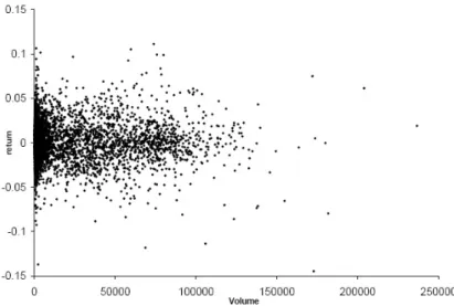
Figure 3.1: Relationship between trade volume and return
frame, e.g. daily. The basic sequential trade model has one trade quantity in each trade. Trades in the real markets, of course, occur in varying quantities. The trade volume is an important market dynamics. To get a preliminary impression about trading volume and stock return, we obtain 10 randomly chosen firms, data from Jan 1988 to Dec 2004 from CRSP database, and plot the cross-sectional daily stock return over daily trade volume in Fig. 3.1. The summary statistics is shown in table 3.1.
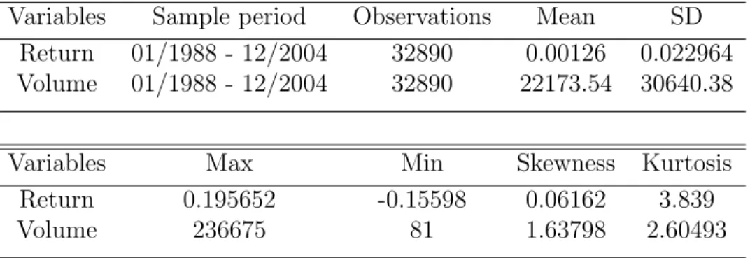
Table 3.1: Summary statistics of daily returns vs. daily volume Variables Sample period Observations Mean SD
Return 01/1988 - 12/2004 32890 0.00126 0.022964 Volume 01/1988 - 12/2004 32890 22173.54 30640.38
Variables Max Min Skewness Kurtosis
Return 0.195652 -0.15598 0.06162 3.839
Volume 236675 81 1.63798 2.60493
From Fig. 3.1, we know that volume are quite symmetric across zero return and high volume does not tend to be associated with high return. In Kyle’s strategic trading model, the author conjectures a relationship between a firm’s stock price change and its order flow. In Pasquariello and Vega (2009) empirical study, they address cross-trading effect with daily aggregated order imbalance. Chordia and Subrahmanyam (2004) show that the total number of transactions has greater explanatory power for stock-return fluctuation than trading volume. We will take similar approach with modified setting. The intuition is that total trade volumes can be decomposed into sell orders and buy orders, it is the order imbalance between sell and buy orders which drive the market movement.
2001 as a starting point. First, we filter the TAQ data by deleting small number of traders and quotes representing possible data error (e.g., negative prices or quotes). We then assign the trades using the following procedure.
1. If a transaction occurs above (or below) the prevailing mid-point of bid-ask spread at that particular time, we assign buy (or sell) sign to that transaction.
2. If the transaction price is at the mid-point of the spread, we will label it a buy (or sell) if the sign of the last trade price change is positive (or negative).
We define the trade direction variable as +1 (buy) or -1 (sell) for each transaction, similar to the Roll model. Then we get the signed order flow by multiple trade direction and order size, denote as ˆ∆yt, where ∆yt = ∆xt+ ∆ut in Kyle’s setting.
We denote order imbalanceas the total number of signed order flows at given time period, e.g. daily. We would expect the signed order flows or order imbalance have greater explanatory power.
3.2
Trade direction
We use{qt}, +1 (buy) or -1 (sell), t= 1,2... to denote intraday trade directions as we
did in the previous chapter. In the Roll model,qt has equal probability, which implies
E(qt|Ft−1) to get zero in the empirical study. Each trading date has one series of high
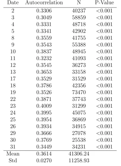
frequency trade directions. We got intraday estimates of the first-order autocorrelation of this high frequency series ˆρk = Corr( ˆqt,qtˆ−k), with k = 1. Table 3.2 shows MSFT
first-order autocorrelation for intraday trade directions in Jan 2001.
In table 3.2, the first column is the trading date. Within each trading date, we got positive correlation between {qt} and {qt−1} as shown in the second column. The
Table 3.2: Sample first-order autocorrelation of trade direction Date Autocorrelation N P-Value
2 0.3306 40237 <0.001
3 0.3049 58859 <0.001
4 0.3331 48718 <0.001
5 0.3341 42902 <0.001
8 0.3559 41755 <0.001
9 0.3543 55388 <0.001
10 0.3837 48945 <0.001
11 0.3232 41093 <0.001
12 0.3545 36273 <0.001
13 0.3653 33158 <0.001
17 0.3529 31529 <0.001
18 0.3786 42356 <0.001
19 0.3526 73470 <0.001
22 0.3871 37743 <0.001
23 0.4009 31299 <0.001
24 0.3995 45075 <0.001
25 0.3954 36869 <0.001
26 0.3934 34915 <0.001
29 0.3666 27078 <0.001
30 0.3769 25538 <0.001
31 0.3449 34231 <0.001
Mean 0.3614 41306.24
Std 0.0270 11258.93
mean 0.3614 and standard error 0.027.
These results have meaningful empirical implications. First, the assumption of the Roll model is not valid in practice. The sequence of the order types are more likely to pair with each other, buy after buy, sell after sell. Secondly, this may imply the asymmetric information processed by difference traders, since the informed traders always trade in the direction of his knowledge. Finally, this explains how day traders could make money by following the market. The daily order flows have high probability to be in the same trade directions sequentially. We would like to address this finding in our statistical inference.
autocorrelation, it is not significant against zero hypothesis. The order sizes are indeed exogenous along the time horizon (e.g. 500 size order could be followed by another 10 or 2000 size order).
3.3
Asymmetric information
In G-M model, the asymmetric information isµ, the proportion of the informed trader in the population. The asymmetric information parameterµis positively correlated to pk(sell), and the bid-asked spread from the previous chapter. These results suggest use
of the bid-ask spread or the impact of an order has on subsequent prices as proxies for the asymmetric information. We study the intraday bid-ask spread movement across one year.
Figure 3.2: MSFT intraday bid-ask spread movement
period (i.e., one week).
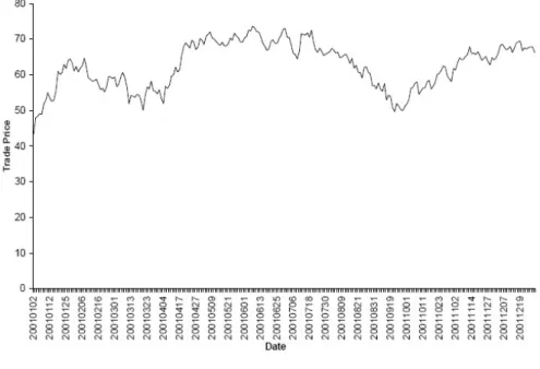
On the other hand, we look at the trade price movement vs. the bid-ask spread. Fig. 3.3 illustrates the trade price movement in corresponding year. The bid-ask spread does
Figure 3.3: MSFT trade price movement
not have strong correlation with the trade price either positively or negatively. The spread contains dealer’s posterior inference about the degree of informed traders, and this measurement is constant at short period. In Fig. 3.2 and 3.3, dealer’s posterior beliefs about the degree of asymmetric information is decreasing, therefore we have seen higher spread in January-April than later the same year, while the trade price still move upward or downward in both directions.
3.4
Market depth
The market depth is an important characteristics of market dynamics. It refers to the size of an order flow innovation required to change the price in a given amount. In Kyle’s framework, the market depth is λ−1
n , with pn =pn−1 +λn∆Yn for n = 1, ..., N.
It deals with order imbalance with respect to the price increment. We do empirical studies at intraday transaction level.
First, we present the aggregated intraday transaction level order imbalance across trade price increments. Figure 3.4 illustrates MSFT aggregated order imbalance vs. price changes at each trading date using microstructure data. The correlation between
Figure 3.4: Aggregated intraday order imbalance vs. price change
the two series is 0.76. The results show strong explanatory power of order imbalance in the price change movement.
We conjecture the market depth (orλn) is constant in Kyle’s model. We use
Figure 3.5: Line fit with market depth (or λn)
The empirical results show that the market depth could be modeled with the intro-duction of order imbalance or signed order flow. These findings have significant impact on the model inference.
3.5
Market liquidity
In the previous section, we considered the liquidity parameter λ, and the results show that demanding liquidity has a cost. Intuitively, if you demand high liquidity, the price would be high. In Kyle’s single period trading model, theλ takes following form:
λ=
√
Σ0
2σ , (3.1)
√
Σ0/σ is ratio of volatilities, i.e., the value uncertainty vs. the noise order uncertainty.
Therefore, theλ ∆Y is like a liquidity risk, where ∆Y is the total order imbalance.
λ ∆Y =
√
Σ0
2 ∆Y
σ , (3.2)
∆Y /σ is proportional to the percentage of order imbalance. The higher σ, the lower the price impact. It is scaled by the value uncertainty √Σ0. The higher the security
value uncertainty, the higher the price impact.
The factor model starts with Fama and French (1992), which shows that factors related to company size and BtoM (Book to Market) ratio are able to explain a signifi-cant amount of the common stock variation in stock returns. They run the three-factor model of the form:
Fama and French 3-factor
Rjt−Rft=αj+βj (Rmt−Rft) +γj SM Bt+ξj HM Lt+jt, (3.3)
where Rjt is the return to portfolio j for time t, Rft is the risk-free return for time t.
SM Bt is the small cap stock vs big cap stock, and HM Lt is the high BtoM stocks vs
Chapter 4
Liquidity in market microstructure
models
4.1
Liquidity and expect returns
Financial markets deviate from the perfect-market ideal in which there are no impedi-ments to trade. A large and growing body of work has identified a variety of market im-perfections, ranging from information asymmetries, participation costs, different forms of trading costs, inventory risk(i.e., the market maker, being exposed to the risk of price changes while he holds in inventory, requires compensation), to search frictions(i.e., a tradeoff between search and quick trading at a discount) etc. These cost of illiquidity
We start the overview with different liquidity measures, and explore the effect of liquidity on assets expected returns by empirical evidence. The literature on liquidity is vast. Madhavan (2002), Bias, Glosten and Spatt (2005), Cochrane (2005), Vayanos and Wang (2009) have surveyed on liquidity and asset prices. While the effects of imperfections on market liquidity and further on expected returns have received much attention, their focuses are expected returns and mostly based on factor models, i.e, adjusted CAPM, adjusted Fama-French models etc. We then distinguish our work from those related literature such that we study the origins of illiquidity(e.g., in the form of bid-ask spreads or market impact) and fundamentals of the imperfections on the price movement with high frequency microstructure data.
4.2
Liquidity measures
One strength of a frictionless economy is that a security’s cash flows and the pricing kernel are sufficient statistics for the pricing operation described as:
pt=Et{ (pt+1+dt+1)
mt+1
mt
}. (4.1)
wheremt is the stochastic discount factor,dt is the dividend process. Equation (4.1) is
the main building block of standard asset pricing theory. The assumption of frictionless market is combined with no arbitrage, agent optimality and equilibrium. No arbitrage
means that one can not make money in one state of nature without paying money in at least one other state of nature. Agent optimalityderives investor’s optimal portfolio choice only on a solution in the absence of arbitrage. If the investor’s preferences are represented by an additively separable utility function EtPsus(cs) for a consumption
process c, then mt = u0t(ct) is the marginal utility of consumption. In a complete
equilibrium, (4.1) is satisfied with utility function ut =
P
iλ iui
t where λi is the Pareto
Weights and depend on agents’ endowments. In a frictionless market, the assumption of no arbitrage is essentially equivalent to the existence of a stochastic discount factor. That means the pricing kernel summarizes all the needed information contained in utility functions of agents, endowments, correlation with other securities etc.
In an economy with frictions, the price depends additionally on the security’s liq-uidity and the liqliq-uidity of all other securities. In some liqliq-uidity models, there still exists a pricing kernel m such that (4.1) holds. In this case, illiquidity affects mt, but
the pricing of securities can still be summarized using a pricing kernel. The empirical analysis of Pastor and Stambaugh(2003) is based on an assumption that there exists anm that depends on a measure of aggregate illiquidity. In other models of illiquidity, however, there is no pricing kernel such that (4.1) applies. For instance, in transaction-cost-based models, securities with the same dividend cash flows have different prices if they have different transaction costs. Hence, a security’s transaction cost not only affects the nature of market equilibrium, it is the fundamental attribute of the security. If there does not exist a pricing kernel, the general equilibrium prices with illiquidity may depend on the fundamental parameters in a complicated way that does not have a closed-form expression. Nevertheless, we still can get important insight into the main principles how liquidity affects assets expected return under certain assumptions and with the assistance of empirical studies.
Consequently, researchers requires a long time series to increase the power of the tests. In stock market outside U.S., high frequency data are hardly available, researchers need to find other measures of liquidity using low-frequency data, such as daily return data, and trading volume etc. The empirical studies from related work employ various measure of liquidities.
4.2.1
Bid-ask spread
Amihud and Mendelson(1986) studies the liquidity on stock’s expected return using quoted bid-ask spreads. These predictions are tested using stock returns over the period 1961-1980 and data on quoted relative spreads. The spreads are the average of the beginning- and end-of-year end-of-day quotes, collected from Fitch quote sheets for NYSE and AMEX stocks. The estimation model is:
Rj =a+b βj+c ln(Sj). (4.2)
whereRj is the monthly stock portfolio return in excess of the 90-day Treasury Bill rate,
βj is the systematic risk, estimated from the preceding period, and Sj is the relative
bid-ask spread. All coefficients are significant.
Figure 4.1: Relationship between stocks’ excess monthly returns and bid-ask spreads
While on NYSE and AMEX, individual investors could trade through limit orders that had priority over the specialist’s quotes and thus avoid the cost of spread although incurring the cost of risk and delay, on Nasdaq trading are done mostly through mar-ket makers, and investors have to endure the cost of spread. The estimated effect of the bid-ask spread is expected to be stronger when using Nasdaq stocks than NYSE and AMEX. This is shown in Eleswarapu(1997), who estimates a model where stock return is regressed on the stock’s beta, relative spread and log(size). The estimation is performed for individual stocks employing Fama and MacBeth method. The consistent significant effect is the relative spread which has positive effect.
4.2.2
Kyle’s
λ
Chordia et al. named it ”theory-based” illiquidity as it originates from Kyle’s frame-work.
Brennan and Subrahmanyam(1996) estimate λ by regressing the price change, on the transaction size. The slope coefficient from the regression is Kyle’sλwhich measures the price impact of a unit of trade size, being larger for less liquid stock. The regression model also includesφ =Dt−Dt−1, where Dt= 1 for a buy transaction and Dt= −1
for a sell transaction. The coefficient of this differential, φ, reflects the fixed cost of trading that is unrelated to the order size. The illiquidity variables that are used are: (1) Cq = λ q/P, the average of the marginal cost of trading, where q and P are
monthly averages of trade size and price. (2) φ/P, the relative fixed cost of trading. These measures of illiquidity are then used in a cross-section regression of monthly NYSE stock returns for the years 1984-1991. The regression model employs Fama and French (1992) three factors model in addition to the illiquidity variables: The market return index, the small-minus-big firm return indexes and high-minus-low book-to-market return index.
The results show thatCq have a positive and significant effects on returns adjusted
by Fama-French factors. In addition,C2
q has a negative and significant effect, consistent
with Amihud and Mendelson (1986) clientele effect that generates an increasing and concave relationship between returns and illiquidity costs.
Chordia, Huh and Subrahmanyam (2009) consider the illiquidity λ in Kyle-type framework with extension to N informed traders and each informed traderiobserves a signal with an errori, i= 1,2, ...N, wherei ∼N(0, v). The asset payoff isW = ˜W+δ,
where ˜W is expected payoff, and δ ∼ N(0, vδ). The informed traders maximize their
size, z ∼N(0, vz). The author shows the Kyle’s measureλ is given by:
λ= vδ
(N + 1)vδ + 2v
s
N(vδ+v)
vz
. (4.3)
where N is the number of informed traders. vδ is the variance of the asset payoff,
vz is the variance of uninformed trades, v is the variance of signal innovation. Note
that this measure requires proxies, for instance, a proxy for the variance of the signal innovation, as well as that of the signal itself. Each of those variance is represented by different proxies. vδ is proxied through the earnings volatility from the most recent
eight quarters. v is proxied by the earnings surprise defined as the absolute value of
the current EPS minus the EPS forecast four quarters ago. vz is proxied by the average
daily dollar volume (in million dollars) within the previous month.
The main model is still multi-factor model. The key contribution is that it uses Kyle’sλto derive a liquidity measure and to establish the connection between liquidity and expected returns.
4.2.3
Daily returns, trading volume and ILLIQ
Researchers often use alternative measures based on daily data on volume, shares out-standing, and prices, which are available for most markets.
can be inferred from the average holding period of the stock, which is the reciprocal of the stock turnover. Datar et al. estimate the cross-section of NYSE stock returns on stock returns in years 1963-1991, controlling for size, book-to-market ratio and beta, employing the Fama and MacBeth method. The result is that the longer the average holding time which implies lower liquidity, or low turnover, the high the expected return.
Amihud (2002) examines the effect of illiquidity on the cross-section of stock returns using an illiquidity measure calledILLIQ, where ILLIQ=|R|/(P ∗V OL), where R is daily return, P is the closing daily price and V OL is the number of shares traded during the day. Intuitively,ILLIQ reflects the relative price change that is induced by a given dollar volume, which is related to Kyle’s pricing impactλ, but on a daily basis.
4.3
Liquidity risk
Liquidity varies over time which means the investors are uncertain what transaction cost they will incur in the future. Secondly, since liquidity affects the level of prices, liquidity fluctuations can affect the asset volatility itself. For both reasons, liquidity fluctuations constitute a new level of risk that impact the fundamental risk. This section explores liquidity models of the effect of a security’s liquidity risk on its expected returns.
Acharya and Pedersen (2005) presents a model which gives rise to a ”liquidity-adjusted CAPM” model that shows how liquidity risks are captured by three liquidity betas, and how shocks affect future expected returns. Re-writing the one-beta CAPM in net returns in terms of gross returns, we get a liquidity-adjusted CAPM for gross returns. Acharya and Pedersen introduce three liquidity betas, βL1, βL2, βL3.
Et(rti+1) =r
f
+Et(cit+1) +λt(βt+βtL1−β L2
t −β L3
where λt =Et(rMt+1−ctM+1−rf) is the risk premium. Et(cit+1) is the expected relative
illiquidity cost. The models states that the required excess return is the expected relative cost plus four betas times the risk premium.
The first liquidity beta βL1
t measures the covariance between the asset’s illiquidity
and the market illiquidity. The model implies the expected return increases with this covariance, because investors want to be compensated for holding a security that be-comes illiquid when the market in general bebe-comes illiquid. The second liquidity beta βtL2 measures the exposure of asset i to marketwide illiquidity, which is usually nega-tive. This beta affects return negatively because investors are willing to accept a lower return in times of market illiquidity. The more negative the exposure to the market illiquidity, the greater is the expected return. The third liquidity betaβL3
t measures the
Chapter 5
Inference on an Extended Kyle’s
Model
This work begins with the celebrated strategic trade model in Kyle (1985). It aims at fitting a modified version of Kyle’s model using some intra-day data, and retaining its interpretability. Our study consists of three parts:
[1] an alternative characterization of the equilibrium solution to Kyle’s model;
[2] derivation of the equilibrium solution to an extended Kyle’s model in which the informed trader observes a noisy signal of the asset value;
[3] A case study of simulated equilibrium solutions.
[4] MCMC dynamic Bayesian inference on a proposed extension of Kyle’s model in the next chapter.
Kyle (1985) proves the existence and uniqueness of a linear equilibrium solution in which the parameters are derived via a set of recursive formulas. In Part [1], we provide a new method to reproduce those parameters. Our method is computationally more convenient and direct. It also paves a road for deriving equilibrium solutions to certain extended models. One extension is analyzed in Part [2], in which the informed trader observes a noisy signal of the asset value v instead of vitself. In Part [4], we perform Bayesian inference on an extended model based on real microstructure data.
5.1
New derivation of Kyle’s equilibrium solution
Recall the basic framework and major result in Kyle (1985).
• Fix an asset in what follows. Suppose N auctions take place sequentially over a trading period (e.g. day, month, year). For each n = 0,1, . . . , N, tn denotes the
•There is a single informed trader who knows the liquidation valuev of the asset, and trades a quantity ∆xn at the nth auction. However, v ∼N(p0,Σ0) is considered
as a random variable by (uninformed) noise traders.
• The quantity traded by noise traders at the nth auction is denoted by ∆un ∼
N(0, σ2
u∆tn) with ∆tn = tn−tn−1. Assume ∆u1, ...,∆uN are independent, and
they are also independent ofv.
•Let ∆yn= ∆xn+ ∆un be the batch order at the nth auction, and FnU−1 denote the
information set available to uninformed traders (including a market maker and all noise traders) at the beginning of the nth auction, consisting of the observations
{p1, ..., pn−1; ∆y1, ...,∆yn−1}, wherepi represents the asset’s market clearing price
determined at theith auction.
• The informed trader (insider) has a richer information set available to him before making his move at thenth auction. Such a setFI
n−1 includes{∆x1, ...,∆xn−1;v}
in addition to FU
n−1. The insider chooses ∆xn based on FnI−1.
•After the move made by the insider at thenth auction, the market maker determines the price pn based on FnU−1 and ∆yn.
•Let
πn = N
X
i=n
(v−pi)∆xi (5.1)
be the total (future) profits of the insider to be made at auctions n, n+ 1, ..., N, and X = (∆x1, ...,∆xN), P = (p1, ..., pN) denote the insider’s trading strategy
and the market maker’s pricing rule respectively. Hence πn=πn(X, P).
(C1) (profit maximization) For n= 1, ..., N and allX0 = (∆x01, ...,∆x0N) with∆x0i = ∆xi, i= 1, ..., n−1, we have
E[πn(X, P)|FnI−1]≥E[πn(X
0
, P)|FI
n−1]. (5.2)
(C2) (market efficiency) For n= 1, ..., N we have
pn=E(v|FnU−1,∆yn). (5.3)
Definition 4. A sequential auction equilibrium (X, P) is called a linear equilibrium if the component functions of X and P are linear, and a recursive linear equilibrium if
there exist parameters λ1, ..., λN such that
pn=pn−1+λn∆yn, n = 1, ..., N. (5.4)
The following theorem is the major result in Kyle (1985) which proves the existence and uniqueness of linear equilibrium, and characterizes those modeling parameters in it.
Theorem 2. There exists a unique linear equilibrium(X, P), represented as a recursive linear equilibrium, characterized by (for n= 1, ..., N)
∆xn = βn (v−pn−1) ∆tn, (5.5)
pn = pn−1+λn∆yn, (5.6)
Σn = V ar(v|FnU), (5.7)
GivenΣ0 andσu2, the parameters βn, λn,Σn, αn, δn are the unique solutions to equations
αn−1 = [4λn(1−αnλn)]−1, (5.9)
δn−1 = δn+αn λ2n σ
2
u ∆tn, (5.10)
βn ∆tn = (1−2αnλn) [2λn(1−αnλn)]−1, (5.11)
λn = βn Σn σu−2, (5.12)
Σn = (1−βnλn ∆tn) Σn−1, (5.13) subject to αN =δN = 0 and the second order condition
λn(1−αnλn)>0. (5.14)
5.1.1
The original derivation of Kyle’s solution
As is suggested on page 1325 in Kyle (1985), combining (5.11) and (5.12) yields
(1−λ2nσ2u∆tn/Σn)(1−αnλn) =
1
2, (5.15)
which is a cubic equation inλn, given nonnegative values of αn, Σn and σ2u. (5.15) has
three real roots. The middle one is the only solution that satisfies the second order condition. Overall, the sequences {λn},{βn},{αn},{δn} and {Σn} can be determined
by iterating n = N, N − 1, ...,1 backwards, given a pair (Σ0, σu2) and the boundary
condition αN = δN = 0. Since ΣN is also unknown, we have to set an initial value
arbitrarily and run a search until it converges. The detail is given as follows.
Given Σ0, σ2u and the boundary condition αN = δN = 0, an iterative algorithm
consists of the following steps:
S2: GetλN =
√ Σ∗
N
σu
√
2∆tn using αN = 0 and (5.15);
S3: Setn=N;
S4: Getβn and Σ∗n−1 from (5.12) and (5.13);
S5: Getαn−1 from (5.9);
S6: Solve the cubic equation (5.15) and use its middle root forλn−1;
S7: Replacen byn−1 and go to S4 if n >0;
S8: If |Σ∗0 −Σ0| > where is a prescribed error bound, go to S2 with a different
initial value Σ∗N, and repeat ...
This backward induction search algorithm contains an outside loop and an inside loop: the outside loop, as shown in S1 — S8, determines Σ∗N up to an acceptable error, while the inside loop solves a cubic equation for each n in S6. Even for a fixed pair (Σ0, σu2), the computational complexity for a desirable target result is O(N2). However,
we can only fix (Σ0, σ2u) in a simulation study. In an empirical study using real market
data, Σ0 and σ2u have to be treated as unknowns and estimated. Conceivably, the
required computational complexity for that task will increase rapidly and make the algorithm impractical. That is why we propose the following alternative algorithm, which is more efficient and has not been explored, to the best of our knowledge.
5.1.2
An alternative characterization of Kyle’s solution
Proposition 1. Assume the same conditions in Theorem 2 with ∆tn= N1 ∀ n, and let
dn = αnλn. Then for every n =N, N −1, ...,1 (running backwards and in particular,
dN = 0 follows from αN = 0), there exists a unique real root dn−1 ∈ (0,1/2) for the cubic equation
where
Kn =
1 1−2dn
. (5.17)
Other parameters in Theorem 2 are determined iteratively by
Σn =
1 2(1−dn)
Σn−1, (5.18)
λn =
(1−2dn) Σn
2(1−dn)∆tn σ2u
1/2
, (5.19)
βn =
1−2dn
2λn (1−dn)∆tn
. (5.20)
Furthermore, the sequence {dn} satisfies the property
1
2 > d1 > d2 >, ..., > dN−1 > dN = 0. (5.21) The sequence {dn} plays a central role in obtaining other parameters in Kyle’s
model. dn has two factors: αn as the coefficient for a quadratic utility function
repre-senting the expected future (at auctionsn, n+ 1, ..., N) profit from the informed trader; andλnas a measure for the market depth (a smaller value ofλncorresponds to a deeper
market). There is another important parameter βn, which models the informed
trad-ing intensity. The followtrad-ing proposition, derived from Proposition 1, depicts how the sequences{βn} and {λn} will evolve as more auctions take place.
Proposition 2.
βn
βn−1 ,
hn =
s
2(1−dn−1)
1−2dn
1−2dn−1
>1 (5.22)
λn
λn−1 ,
kn =
s
1−2dn
1−2dn−1
1−dn−1
2(1−dn)2
> 1
2. (5.23)
Remark: There are several advantages for the proposed algorithm given in Proposition 1.
•Computational efficiency: With this algorithm, the cubic equation (5.16) only need to be solved for eachnonce for all, i.e. it does not depend on the values of Σ0 andσu2.
Therefore, this part of computation is purely off-line. Having solved for the entire sequence dn, n = N −1, ...,1, we can run a forward algorithm, with n = 1, ..., N
and an assigned pair (Σ0, σu2) to obtain other sequences{λn},{βn},{αn},{δn}and
{Σn}. Suppose we have done the calculation for a given N, and decide to run it
again for a larger N0 > N. Then we can reuse the result of dN, dN−1, ..., d1 for
dN0, dN0−1, ..., dN0−N+1, and continue to calculate only new values fordN0−N, ..., d1. Moreover, the only computational errors involved in the new algorithm come from numerical solutions for (5.16). No “trial-and-error” with different values for Σ∗N in the previous numerical search is required. The greater value of N, the more efficient the new algorithm will be.
•From Proposition 2, we learn that the informed trader increases his orders as more auctions take place. As trading unfolds and more information is released to him, the insider has no incentive to hide his private information hence trades more aggressively. Following our derivation, neither ratio βn/βn−1 nor ratio λn/λn−1
depend on any other parameters in the model, except for the auction horizon N. However, the initial values β0 and λ0 do depend on the inputs Σ0 and σu2
[see (5.12)], and such dependence will carry on in subsequent values βn and λn.
Once the sequence {dn} is solved, ratios for both sequences will be uniquely
determined. Moreover, the sequence {βn} exhibits a consistent growth, while λn
does not reveal this property.
Kyle’s model in parameter estimation with real data. The new algorithm turns out to offer a useful clue for what extensions we may consider. We will elaborate on that part in the next section.
Figure 5.1 demonstrates the numerical results of {dn} sequence given number of
periodsN. {dn}is a decreasing sequence as we expect. It also shows that the beginning
portion of{dn}sequence are concentrated within the range of 0.45−0.5 when the total
number of periods N >10. WhenN is large, {dn} would be decreasing slowly for the
majority of time periods, and drop sharply at the end of trading.
Figure 5.1: {dn} series with various sample periods N
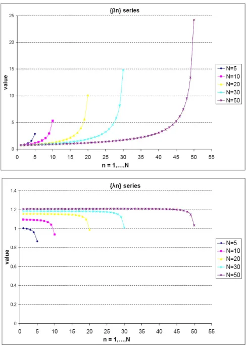
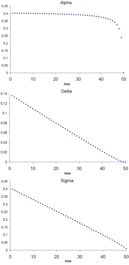
We illustrate the patterns ofλnandβnin figure 5.2 given same initial condition with
different sample periodsN. βnrepresents the insider’s strategy whileλnis the reciprocal
of market depth. βn is an increasing sequence under Kyle’s equilibrium model, and it
follows a pattern of flat at the beginning and gradually more steep toward the end of trading periods. If we compare βn across different N, the results are favorable to the
over longer periods. The λn sequence is at no surprise. It flattens out through the
entire time horizon, and drop at the end of trading periods.
at each auction
5.2
An extension of Kyle’s model
In this section, we consider an extended Kyle’s model in which the informed trader observes a noisy signal about true value v at each auction, but not v itself. We will focus on the case of sequential (multiple) auctions after skimming over the single period case.
5.2.1
The single period case
Consider an asset with payoff v ∼N(p0,Σ0). The quantity traded by noise traders is
denoted by u ∼ N(0, σ2
u). Different from the original Kyle’s model, here we assume
the informed trader observes a signal s = v + at the beginning of the period where ∼ N(0, σ2
). Conditioning on s, the informed trader maximizes his expected profit
by choosing his trading strategy x. Assume that v, u, and are independent of each other. There is a competitive risk-neutral market maker, who sets the asset price as p(y) =E(v|y) based on the batch order y=x+u.
Lemma 1. There exists a unique equilibrium (X, P), in which the insider’s trading strategy X and the market maker’s pricing rule P are linear functions of s and y
respectively:
x(s) = β (s−p0), (5.24)
where
λ = Σ0
2pσ2
u(Σ0+σ2)
, (5.26)
β =
s
σ2
u
Σ0+σ2
. (5.27)
Proof: Let π = [v −p(y)] x. Following the linearity assumptions (5.24), (5.25) and conditioning on the signals, the informed trader will choose x=x(s) to maximize his expected profit
E(π|s) = E[(v−p0−λy) x|s]
= x E(v−p0|s)−x λ E(x+u|s)
= x E(v−p0|s)−λ x2, (5.28)
where the projection theorem implies
E(v−p0|s) =
Cov(v −p0, s)
V ar(s) (s−Es)
= Σ0
Σ0+σ2
(s−p0)
= γ (s−p0), (5.29)
with
γ = Σ0 Σ0+σ2
. (5.30)
MaximizingE(π|s) with respect to x leads to −2λx+E(v−p0|s) = 0, hence
with
β = γ
2λ. (5.32)
Furthermore, the projection theorem and (5.25) imply
p(y) = E(v|y)
= p0+
Cov(v, y)
V ar(y) (y−Ey)
, p0+λ y, (5.33)
and
λ = Cov(v, β (v−p0+) +u) V ar(y)
= βΣ0
β2 (Σ
0+σ2) +σ2u
. (5.34)
Therefore, (5.26) and (5.27) follow from (5.30) and (5.32). Moreover,
E(π|s) = Σ0
p
σ2
u
2(Σ0+σ2)3/2
(s−p0)2.
The ex-ante profit for the insider is given by
E(π) = Σ0
p
σ2
u
2 (Σ0+σ2)1/2
. (5.35)
The special case with = 0 will return to the original Kyle’s solution, i.e., λ= 12qΣ0
σ2 u
and β =
q
σ2 u
Σ0. Note that the noisy signal reduces the insider’s profit compared to the