DETECT COPY NUMBER VARIATIONS FROM READ-DEPTH OF HIGH-THROUGHPUT SEQUENCING DATA
Weibo Wang
A dissertation submitted to the faculty of the University of North Carolina at Chapel Hill in partial fulfillment of the requirements for the degree of Doctor of Philosophy in the Department of
Computer Science.
Chapel Hill 2015
Approved by: Wei Wang Wei Sun
© 2015 Weibo Wang
ABSTRACT
Weibo Wang: Detect Copy Number Variations from Read-depth of High-throughput Sequencing Data
(Under the direction of Wei Wang)
Copy-number variation (CNV) is a major form of genetic variation and a risk factor for various human diseases, so it is crucial to accurately detect and characterize CNVs.
High-throughput sequencing (HTS) technologies promise to revolutionize CNV detection but present substantial analytic challenges. This dissertation investigates improving the CNV detection using HTS data mainly from the following aspects.
• It is observed that various sources of experimental biases in HTS confound read-depth estimation, and bias correction has not been adequately addressed by existing methods. This dissertation presents a novel read-depth-based method, GENSENG, which identify regions of discrete copy-number changes while simultaneously accounting for the effects of multiple confounders.
• It is conceivable that allele-specific reads from HTS data could be leveraged to both enhance CNV detection as well as produce allele-specific copy number (ASCN) calls. Although statistical methods have been developed to detect CNVs using whole-genome sequence (WGS) and/or whole-exome sequence (WES) data, information from
allele-specific read counts has not yet been adequately exploited. This dissertation presents an integrated method, called AS-GENSENG, which incorporates allele-specific read counts in CNV detection and estimates ASCN using either WGS or WES data. • Although statistically powerful, the GLM+NB method used in GENSENG and
ACKNOWLEDGEMENTS
First of all, I would like to express my sincere gratefulness to my advisor Dr. Wei Wang for her continuous guidance and support. I feel especially fortunate to have worked closely with Dr. Jin Szatkiewicz and Dr. Wei Sun who encouraged me to work persistently, and greatly helped me to improve my critical thinking ability and writing skill. Special thanks go to Dr. Jan Prins who chaired my committee and provided assistance to me. I would also like to thank Dr. Leonard McMillan who served on my committee and devoted a lot of effort to my study.
My special thanks also go to members in CompGen Lab, including Eric Yi Liu, Zhaojun Zhang, Shunping Huang, Wei Cheng, etc., for their thoughtful discussions on the problems in the research. I would like to thank all fellow persons I met in the Computer Science department who provide all kinds of help to me during my entire pursuit of PhD. I would also like to thank all the warm-hearted persons I met in the past few years for helping me to live here in Chapel Hill, the beautiful town in North Carolina.
TABLE OF CONTENTS
LIST OF TABLES . . . x
LIST OF FIGURES . . . xi
1 INTRODUCTION . . . 1
1.1 Background . . . 1
1.1.1 Significance of Detecting Copy Number Variation . . . 1
1.1.2 CNV Detection Methods based on High Throughput Sequencing Data . . . 2
1.1.3 Computational Burden in the Read-count based CNV Analysis . . . 6
1.2 Thesis Statement . . . 7
1.3 Summary . . . 9
2 GENSENG . . . 11
2.1 Overview . . . 11
2.2 Materials and Methods . . . 12
2.2.1 Datasets included in this study . . . 12
2.2.2 Input data preparation for CNV detection . . . 14
2.2.3 Overview of the GENSENG method . . . 16
2.2.4 CNV detection method . . . 19
2.2.5 Performance assessment . . . 24
2.3 Results. . . 27
2.3.1 Evaluation of experimental biases in HTS . . . 27
2.3.2 Performance assessment and comparison . . . 31
2.4 Discussion . . . 45
3 AS-GENSENG . . . 47
3.1 Overview . . . 47
3.2 Materials and Methods . . . 48
3.2.1 Method summary . . . 48
3.2.2 Data preparation . . . 51
3.2.3 Hidden Markov model . . . 59
3.2.4 Inference of ASCN in WES data . . . 63
3.2.5 Performance Evaluation: WGS data. . . 64
3.2.6 Performance Evaluation: WES data . . . 67
3.2.7 CNV validation using NanoString technology . . . 71
3.3 Results. . . 72
3.3.1 CNV detection in whole-genome sequencing-simulation data . . . 72
3.3.2 CNV detection in whole-genome-sequencing real data . . . 74
3.3.3 CNV detection in whole-exome sequencing-simulation data . . . 77
3.3.4 CNV detection in real whole-exome-sequencing data . . . 79
3.3.5 CNV validation using NanoString technology . . . 82
3.4 Discussion . . . 84
4 R-GENSENG . . . 87
4.1 Introduction . . . 87
4.2 Methods . . . 88
4.2.1 The consistency of RGE . . . 88
4.2.2 The variance of RGE . . . 92
4.2.3 RGE in a real application . . . 96
4.3 Experiment Results . . . 97
4.3.2 R-GENSENG performance evaluation . . . 100
4.4 Discussion . . . 104
5 CONCLUSIONS . . . 107
LIST OF TABLES
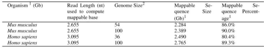
2.1 Fraction of mappable bases in human and mouse genomes . . . 29
2.2 Performance assessment based on simulated sequencing data for a chromosome . . . . 33
2.3 Evaluation of the effects of modeling techniques using NA12878 . . . 34
2.4 Performance assessment based on NA12878 HTS data . . . 35
2.5 Sensitivity to detect deletions in CEU trio data . . . 36
2.6 Performance on datasets with varying sequence coverage: simulation . . . 37
2.7 Performance on datasets with varying sequence coverage: simulation . . . 37
2.8 Summary GENSENG results from the mouse dataset . . . 43
3.1 Allelic configuration correspondences for each HMM state . . . 49
3.2 Methodologies comparisons among WGS methods . . . 65
3.3 Methodologies comparisons among WES methods . . . 68
3.4 Performance comparison on WGS-read-count-simulation data . . . 72
3.5 Performance comparison on WGS-sequencing-read-simulation data . . . 73
3.6 Performance comparison with WGS methods on WGS-simulation data. . . 73
3.7 Performance assessment based on WGS data of two HapMap samples . . . 75
3.8 Performance comparison on WGS simulation down-sampled data . . . 76
3.9 Performance comparison on WGS simulation down-sampled data . . . 77
3.10 Performance comparison on WES-simulation data . . . 77
3.11 Performance comparison with WES methods on WES-simulation data . . . 78
3.12 Performance assessment based on WES-emprical data . . . 80
4.1 Sensitivity with different window size . . . 102
LIST OF FIGURES
2.1 GENSENG flowchart . . . 17
2.2 Example high-confidence CNVs predicted by GENSENG: NA12878 HTS . . . 18
2.3 Relationship between read-depth and known confounders: NA12878 . . . 27
2.4 Relationship between read-depth and known confounders: AKR/J . . . 27
2.5 Read-depth distribution after accounting for known confounders . . . 29
2.6 Relationship between read-depth and mappability in high-confidence CNVs. . . 30
2.7 Illustration of sensitivity and FDR calculation . . . 31
2.8 Example shared deletion identified from the human HTS dataset. . . 40
2.9 Example private deletion identified from the human HTS dataset. . . 41
2.10 Example shared duplication identified from mouse HTS datasets. . . 44
2.11 Example shared deletion identified from the mouse HTS dataset.. . . 45
3.1 AS-GENSENG overview . . . 48
3.2 Jointly analysis by AS-GENSENG . . . 50
3.3 AS duplication example . . . 52
3.4 AS deletion in NA12891 recovered in AS-GENSENG . . . 53
3.5 AS deletion in NA12892 recovered in AS-GENSENG . . . 54
3.6 Example: Common Deletion in WES data . . . 55
3.7 HMM flowchart to infer ASCN . . . 59
3.8 Whole-exome sequencing-simulation flowchart . . . 70
3.9 An example target that AS-GENSENG better estimates expected RC . . . 81
3.10 An example target that AS-GENSENG better estimates expected RC . . . 82
3.11 An example target that AS-GENSENG better estimates expected RC . . . 83
3.12 Example: NanoString nCounter Technology Validation . . . 83
CHAPTER 1: INTRODUCTION
1.1 Background
1.1.1 Significance of Detecting Copy Number Variation
studies. Using genome-wide SNP arrays (Attiyeh et al., 2009; Gardina et al., 2008; Greenman et al., 2010; Pounds et al., 2009), allele-specific intensity signals for two SNP alleles (denoted as alleles A and B) can be obtained and integrated in CNV detection. ASCN calls can then be generated (e.g., A, AAB, BBB, ABBB). ASCN calls provide a more accurate characterization of the underlying DNA sequence of each individual, thereby reducing the rate of apparent Mendelian inconsistencies (McCarroll et al., 2006; Korn et al., 2008) and could improve statistical power for tests of
association with complex diseases(Marenne et al., 2013).
1.1.2 CNV Detection Methods based on High Throughput Sequencing Data
Recent advances in high-throughput sequencing (HTS) (Bentley et al., 2008; McKernan et al., 2009; Wheeler et al., 2008) are promoting whole-genome sequencing (WGS) or
whole-exome sequencing (WES) as an all-in-one high-throughput assay for characterizing
single-nucleotide polymorphisms (SNPs) and CNVs, and could replace microarrays as a discovery platform (Alkan et al., 2011; Medvedev et al., 2009). While microarray-based CNV detection analyzes probe hybridization intensities, HTS-based CNV detection uses conceptually distinctive approaches: read-pair, split-read, and read-depth analyses, which vary in their sensitivity and specificity depending on the sizes and classes of SVs (Mills et al., 2011; Alkan et al., 2011; Medvedev et al., 2009). Converging evidence suggests that multiple approaches should be
considered together to maximize CNV detection from HTS data. For example, the 1000 Genomes Project used 19 algorithms to independently identify CNVs in 185 human genomes and pooled the results according to the specificity of each algorithm (Mills et al., 2011). Recent methods
(SPANNER (Mills et al., 2011), CNVer (Medvedev et al., 2009) and Genome STRiP (Handsaker et al., 2011)) integrate read-pair and read-depth in the detection process in different ways.
The read-depth approach looks for higher or lower than expected sequencing coverage in a genomic region to infer gain or loss of DNA. Read-depth has been computed in a variety of ways, including counting the number of fragments (Handsaker et al., 2011) or reads (Abyzov et al., 2011; Campbell et al., 2008; Yoon et al., 2009; Medvedev et al., 2010) mapped to a particular genomic region and calculating the sum of per-base coverage within a region (Simpson et al., 2009; Sudmant et al., 2010). Existing CNV detection methods assume that read-depth follows a Poisson
distribution (or a normal distribution as the large-sample approximation of the Poisson model) for a diploid genome and search for regions that diverge from this distribution. However, in practice, neither sampling nor mapping of the reads is uniform, because of experimental biases. GC content can lead to certain genomic regions being over- or under-sampled (Bentley et al., 2008). Repetitive DNA elements are abundant in the mammalian genomes (Treangen and Salzberg, 2012);
to trace (e.g., noise arising from sequencing, sequencing errors), create further variability in read-depth coverage. Violation of the assumed Poisson distribution entails loss of
sensitivity/specificity to detect CNVs using read-depth. Thus, when analysing HTS data, it is critical to correct for various sources of experimental bias that distort the quantitative relationship between read-depth and true copy number, hindering the ability for accurate CNV detection (Bentley et al., 2008; Treangen and Salzberg, 2012; Szatkiewicz et al., 2013).
Bias correction has not been adequately addressed in the literature. In studies of cancer, matched pairs of tumor- and normal-tissue samples may be used to correct biases by computing read-depth ratios (Chiang et al., 2009; Xi et al., 2011; Xie and Tammi, 2009; Ivakhno et al., 2010). While cancer studies afford themselves the use of tumour/normal pairs, numerous techniques have been developed for germline CNV studies to normalize read-depth data (a.k.a. correct bias) (Handsaker et al., 2011; Abyzov et al., 2011; Yoon et al., 2009; Medvedev et al., 2010; Simpson et al., 2009; Sudmant et al., 2010; Chiang et al., 2009; Xi et al., 2011; Xie and Tammi, 2009; Wang et al., 2013). For WGS, most existing methods (Abyzov et al., 2011; Yoon et al., 2009; Sudmant et al., 2010) use a two-step approach, where read-depth data from a single-genome is first adjusted to account for the effect of known sources of bias (e.g. GC content) and then the adjusted
methods (Amarasinghe et al., 2013; Nord et al., 2011; Plagnol et al., 2012; Li et al., 2012; Love et al., 2011; Wu et al., 2012; Tan et al., 2014). The PCA/SVD methods assume that most variation observed in the sample-by-target read-depth matrix is due to noise with little contribution from CNVs; and therefore remove several of the strongest variance components for the purpose of noise reduction. In this paradigm, XHMM (Fromer et al., 2012) applies a PCA that is optimized for detecting rare CNVs (frequency<5%), whereas common CNVs could not fit in this model. CoNIFER (Krumm et al., 2012) applies a SVD and removes the first 12-15 variance components for detecting rare CNVs but 5 components for common CNVs. However, as the frequencies of CNVs cannot be known before they are detected, it is challenging to determine how to choose the top-K variance components in order to prevent the PCA/SVD methods from removing true CNV signals (Tan et al., 2014). Alternatively, the reference-set methods create a baseline for each exon target from a reference group of copy number two, where the baseline from the reference set captures technical variation but not variation due to CNVs. Then read-depth ratios of test samples versus the baseline are computed for the purpose of noise reduction (Amarasinghe et al., 2013; Nord et al., 2011; Plagnol et al., 2012; Li et al., 2012; Love et al., 2011; Wu et al., 2012). However, the power to detect common CNVs is often limited, owing to the difficulty in constructing the true reference set in the presence of common CNVs, especially when the CNV frequency is high and unknown (Plagnol et al., 2012; Li et al., 2012). Here we demonstrate that allele-specific read count information can be leveraged to identify the proper reference group of samples with copy number two and this method subsequently improves detection of common CNVs at any frequency.
information has not been extensively explored in the literature. With WGS data, ERDS (Heinzen et al., 2012) is the only existing method that leverage allele-specific information but it has a number of limitations. For example, deletions are detected by simultaneous analysis of read-depth and the total number of heterozygous SNPs followed by refinement of smaller segments (<10kb) using read-pair information; however, duplications are detected using read-depth only. Further, ERDS estimates total copy-numbers but it is not capable of estimating ASCN. For WES data, many effective methods have been developed to estimate rare or common CNVs (Fromer et al., 2012; Amarasinghe et al., 2013; Coin et al., 2012; Karakoc et al., 2012; Koboldt et al., 2012; Nord et al., 2011; Plagnol et al., 2012; Krumm et al., 2012; Li et al., 2012; Love et al., 2011; Wu et al., 2012); however, none of the existing methods leverage allele-specific information in CNV detection or are capable of estimating ASCN. To overcome these deficiencies, here we develop a novel method that uses allele-specific information to aid the detection of both deletions and duplications and is capable of determining ASCN from both WGS and WES data.
1.1.3 Computational Burden in the Read-count based CNV Analysis
The read-depth data (windowed or gene/exon-level read counts) are by nature a series of counts, for which the negative-binomial (NB) distribution has been shown as the suitable
distribution in statistical modeling (Robinson and Smyth, 2008; Anders and Huber, 2010; Rashid et al., 2011b; Szatkiewicz et al., 2013). The NB model is flexible for modeling genomic read-count data because its dispersion parameter allows larger variance and therefore less restrictive than Poisson distribution. Further, via generalized linear models (GLMs) (McCullagh, 1983), the NB model provides a powerful framework to simultaneously account for confounding factors (e.g. genomic GC content and mappability) and determine the true relationships between read-count signals and biological factors (Szatkiewicz et al., 2013).
2012; Robinson and Smyth, 2007, 2008; Zhou et al., 2014) for detecting differential expression using RNA-seq; and ZINBA (Rashid et al., 2011b) for detecting enriched regions using ChIP-seq, DNase-seq, or FAIRE-seq. While statistically powerful, GLM+NB methods encounter a big data problem when applied to genomic read-count data comprised of tens of thousands of
windows/genes/exons. The iterative reweighed least square (IRLS) algorithm is the standard approach to fit GLMs (Green, 1984). IRLS has a quadric complexity with the size of data and needs to be run multiple times until it converges. The expensive computation cost of GLM hinders the computational efficiency of the GLM+NB methods in their applications to genomic read-count data.
1.2 Thesis Statement
Thesis:Accurate and efficient CNV detection based on the analysis of read-depth of HTS
data could be achieved by correcting biases in HTS and leveraging the allele specific information
accompanied with HTS data.
This dissertation presents an integrated likelihood-based CNV inference framework, which is based on Hidden Markov Model (HMM), that combines multiple information along with the read-depth in HTS data to detect CNV. Three specific design aims of the framework are listed below:
• Specific Aim 1:Improve CNV detection accuracy through correcting biases.Biases could
lead to read-depth diverges from expected values and cause false positive CNV calls. However, the effect of biases could be quantified and corrected so that read-depth could be correctly analyzed to achieve more accurate CNV detection.
• Specific Aim 2:Allele specific information could not only be used to generate ASCN, but
also it could lead to accurate CNV predictions. ASCN is highly desirable. The success of
CNV detection in microarray study inspires the incorporation of the allele specific information in HTS based CNV detection.
• Specific Aim 3:The CNV prediction could be both accurate and efficient.The
computation efficiency could be improved by randomly sampling a subset of data before the analysis so that the scale of analysis is reduced. Even so, the accuracy should still be comparable with using all data.
As the support of the thesis statement and the research aims above, the contributions made in the thesis are summarized as follows.
• A method GENSENG is developed that simultaneously corrects biases and segment CNV. HMM is employed to respect the spatial nature of the CNV (consecutive regions tend to have the same copy number). Through evaluation of read-depth data distribution using both human data and mouse data, negative-binomial distribution is found as a better distribution because it captures the characteristics of real data by allowing the variance larger than the mean. A negative-binomial regression is applied, which is a specific case of the generalized linear model (GLM), to quantify the relation between read count, underlying copy number, and biases (GC content and mappability). The
negative-binomial regression procedures emission probability of HMM. HMM generates the posterior probability given each underlying copy number for each window, and based on the posterior probability GENSENG segments CNV. GENSENG achieves higher CNV detection accuracy than its peer methods which do not adequately quantify the effect of biases in terms of sensitivity and FDR.
AS-GENSENG brings ASCN and is capable of detecting CNV from both WGS and WES data. It further improves the CNV detection accuracy over GENSENG and has better accuracy than its WGS companion methods when the size of CNV is larger than1kbps. With the accurate expected read count estimation AS-GENSENG achieves higher accuracy than other WES methods when the CNV frequency is high (common CNV). • In this study, we introduce the randomized GLM+NB coefficients estimator (RGE) for
speeding up the GLM+NB based read-count analysis. Our RGE uses a weighted sampling strategy. To illustrate the utility of RGE, we used our GLM+NB based CNV detection method GENSENG (Szatkiewicz et al., 2013) as an example and named the resulting RGE-GENSENG as “R-GENSENG”. We first evaluated the consistency and the variance properties of RGE. We concluded that RGE is a consistent GLM+NB regression
estimator, and that the weighting sampling strategy applied in RGE yields smaller regression coefficients estimation variance than using uniform sampling. We then performed simulation and real-data analysis to evaluate R-GENSENG in comparison to the original GENSENG. We concluded the R-GENSENG is ten times faster than the original GENSENG while maintaining GENSENGs accuracy in CNV detection. Taken together, our results suggest that RGE and the strategy developed in this work could be applied to other GLM+NB based read-count analyses in order to substantially improve their computational efficiency while preserving the analytic power.
1.3 Summary
In this chapter, I have illustrated the extreme importance of accurate CNV detection and ASCN profiling. With the advance of HTS technology, it is highly demanding to develop
• In Chapter 2, I will present the detailed descriptions of GENSENG method. GENSENG has been validated extensively on both simulation data and real data. I will introduce the simulation procedures as well as the sources of real data in Chapter 2. I will also
introduce the experiments setup and the comparison results of GENSENG with the state of the art methods.
• In Chapter 3, I will present the method characterization of AS-GENSENG. The evaluation of AS-GENSENG is conducted on two different data, WGS data and WES data, respectively, and for each data, both simulation study and real data study are conducted. I will introduce details of the conducted experiment results in Chapter 3. Through extensive comparison with peer methods, AS-GENSENG is concluded to not only predict ASCN, but also improve the CNV detection accuracy. I will introduce the comparisons and bring the discussions.
• In Chapter 4, I will introduce the RGE and the efficiently implemented R-GENSENG. I will first show the properties of the RGE, and show its application R-GENSENG. The properties of RGE are established by both theoretic derivation and simulation validation, which are both covered in Chapter 4. The performance of R-GENSENG on accurate and efficient CNV detection is evaluated on both simulation data and real data. I will present the results in Chapter 4.
CHAPTER 2: GENSENG
2.1 Overview
In Section 1, we have mentioned that bias correction has not been adequately addressed in the literature. Experimental biases would seriously affect the read-depth and leads to false CNV calls. Some existing methods (Abyzov et al., 2011; Yoon et al., 2009; Sudmant et al., 2010) adopt a two-step approach where read-depth is first smoothed for GC content differences using linear regression, and the GC-adjusted read-depth is then segmented. Other methods (Handsaker et al., 2011; Medvedev et al., 2010) account for mapping bias of a candidate region by using its effective length (e.g. the number of confidently mapped bases); however, this approach does not account for the dependence between consecutive regions or additional sources of noise in the data. While various kinds of adjusted read-depth have been used as input, nearly all methods (Handsaker et al., 2011; Yoon et al., 2009; Medvedev et al., 2010; Simpson et al., 2009) employ the Poisson or normal-distribution assumption without subsequent evaluation the adequacy of the distributional assumption.
accommodated by the over-dispersion parameter of the negative binomial distribution and by an additional noise component via a mixture model. Fourth, we calibrate our method using simulation and whole-genome-sequencing data from the 1000 Genomes Project (1000GP) (Mills et al., 2011); and we compare our method to CNVnator (Abyzov et al., 2011), the best-performing
read-depth-based CNV detection algorithm in the literature (Mills et al., 2011). Finally, to demonstrate the utility and robustness of our method, we apply our method to both human and mouse HTS datasets.
In summary, our method outperforms existing read-depth-based CNV detection algorithms and distinguishes homozygous and heterozygous deletions and high-copy duplications. Our method complements the current literature, and the concept of simultaneous bias correction and CNV detection can serve as a basis for combining read-depth with read-pair or split-read in a single analysis. A user-friendly and computationally efficient implementation of our complete analytic protocol is freely available athttps://sourceforge.net/projects/genseng/.
2.2 Materials and Methods
In this section, the studied sequencing datasets are first introduced then followed by the procedure to convert them to read-depth data. After that, a developed CNV detection method GENSENG (Szatkiewicz et al., 2013) is introduced.
2.2.1 Datasets included in this study
1000 Genome Project data. For method development and assessment, we used the
whole-genome sequencing data from 3 HapMap individuals sequenced as part of the 1000 Genomes Project. These include the CEU parent-offspring trio of European ancestry (NA12878, NA12891, NA12892), sequenced to 42x coverage on average using the Illumina Genome Analyzer (I and II) platform. Sequencing reads were a mixture of single-end and paired-end with variable lengths (36bp, 51bp). The complete genome sequence data were obtained in the form of .bam alignment files from
as described in the on-line documentation:
ftp://ftp.ncbi.nlm.nih.gov/1000genomes/ftp/README.alignment_data.
High-confidence CNVsTo assess the sensitivity of our discovery method, we used the
high-confidence CNVs established for NA12878 (Supplementary Table 6 of (Mills et al., 2011)) by combining CNVs reported in earlier surveys that used high-density microarrays (Conrad et al., 2010; McCarroll et al., 2008), fosmid sequencing (Kidd et al., 2008), or ABI tracing mapping (Mills et al., 2006). This dataset included 610 deletions (∼82% from microarray reports (Conrad et al., 2010; McCarroll et al., 2008)) and 261 duplications (100% from microarray reports (Conrad et al., 2010; McCarroll et al., 2008)) from the autosomes of NA12878. The second high-confidence dataset used in this study was generated by Handsaker et al. (Handsaker et al., 2011) by accurately genotyping deletions from the 1000GP HTS data (Mills et al., 2011). The complete dataset was downloaded from
ftp://ftp.broadinstitute.org/pub/svtoolkit/misc/1kg/NGPaper/and included deletions for the 3 aforementioned HapMap individuals. This dataset included 2301 deletions for NA12878, 2200 deletions for NA12891, and 2055 deletions for NA12892. CNV coordinates reported in both high-confidence datasets were translated from NCBI36 to NCBI37 using liftOver.
Data from other sequencing projects. To demonstrate the robustness of our method, we
used HTS data from two different studies using various sequencing platforms, sequencing depths, and read lengths. In the first study, we used the whole-genome sequencing data of 3 individuals affected with bipolar disorder from a large multiplex Spanish pedigree currently under investigation. Paired-end sequencing with 100bp reads was performed at the University of North Carolina on the Illumina HiSeq 2000 platform. Each individual was sequenced to an average of 15x coverage. Reads were aligned to the human reference genome NCBI37 using BWA (Li and Durbin, 2009) (v.0.5.5) with default parameters. In the second study, we downloaded
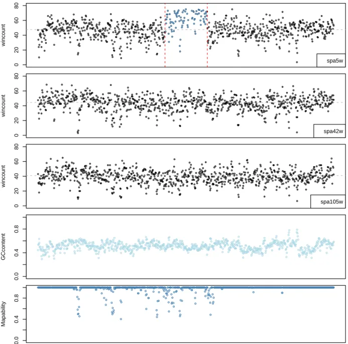
Sanger Institute (Keane et al., 2011). All mouse samples were sequenced on the Illumina GAII platform with a mixture of 54bp, 76bp, and 108bp paired reads to a coverage ranging from 17x to 43x. Reads were aligned to the mouse reference genome NCBI37 using the MAQ aligner (Yalcin et al., 2011; Li et al., 2008). For this study, we analyzed the alignment files for 13 inbred strains (129S1SvlmJ, A/J, AKR/J, BALB/cJ, C3H/HeJ, CAST/EiJ, CBA/J, DBA/2J, LP/J, NOD/LtJ, NZO/HILtJ, PWK/PhJ, WSB/EiJ). We also downloaded the released structural variation (SV) calls for these strains fromftp://ftp-mouse.sanger.ac.uk/current_svs/. These SVs have been classified into several categories based on specific paired-end mapping patterns briefly described in (Yalcin et al., 2011). From this SV release, we extracted 2 categories, including deletions and copy number gains (GAINS and TANDEMDUP), to compare to the
GENSENG-predicted calls.
Reference genomes. The human reference genome NCBI37 was obtained from
ftp://ftp.ncbi.nlm.nih.gov/1000genomes/ftp/technical/reference/ human_g1k_v37.fasta.gz. The mouse reference genome NCBI37 was obtained from ftp://ftp-mouse.sanger.ac.uk/ref/NCBIM37_um.fa.
2.2.2 Input data preparation for CNV detection
Mills et al., 2011)) is represented by its middle base pair. A fragment is counted where read mapping information is available.
1. If two ends of a pair fall in two windows, assign 1/2 to each window where the ends fall; 2. If both ends of a pair fall in the same window, assign 1 to the window;
3. If paired-ended but only one-end present, assign 1/2 to the window where the ends fall; 4. If single-end, always assign 1 to the window where the end falls.
GC content: First we calculate the proportion of G or C bases in each window from a given
reference genome. Then we apply a cubic spline smoothing and transform the GC proportion based on the fitted curve so that the transformed GC proportion and the logarithm of the read-depth are linearly correlated. Finally the transformed GC proportion is median-centered and is referred to as GC content hereafter.
Mappability score: As a function of both reference sequence and read length (K-mer),
mappability score is calculated a priori in four steps: (1) Identify K-mers where each K-mer consists K consecutive bases starting at each base position from the reference genome. (2) Align the K-mers back to the reference genome using a desired aligner, e.g. BWA (Li and Durbin, 2009). Ideally, the aligner and the alignment parameters are chosen to match what was used for generating read alignment files from the sample genomes. (3) Identify mappable base positions where the corresponding K-mers map back to themselves unambiguously (i.e. there is a single best hit and it is the true position of the K-mer). For example, the X0 field produced by BWA (Li and Durbin, 2009) relates a K-mer from a specific place in the genome to the number of best hits of that K-mer in the entire genome. If a K-mer has a X0 value of 1, the corresponding base can be identified as a mappable base. (4) Compute mappability score as the proportion of mappable bases in a given window, which measures the uniqueness of specific regions of the reference genome.
Window consideration: The window size and the degree of overlap between them are
non-overlapping windows would decrease precision in defining CNV breakpoints and miss CNVs that only partially span one window. Third, a higher degree of overlap introduces more
inter-window correlation, which necessitates appropriate adjustment in modeling the RD signals. In summary, the input data is a tuple for each window represent by
{O, X}={o1...oT, x1...xT}, where T is the total number of windows of a
chromosome,otdenotes the read-depth,xt= (gt, lt)denotes the covariates of thetthgenomic region, wheregtrepresents the GC content, andltdenotes the mappability score.
2.2.3 Overview of the GENSENG method
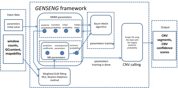
To mitigate the effects of experimental bias and improve read-depth-based CNV detection, we developed a novel statistical method called GENSENG (Szatkiewicz et al., 2013). The unique feature of GENSENG is to integrate the correction of multiple sources of bias and the inference of the copy-number states in a single analysis. Figure 2.1 gives an algorithmic overview of
GENSENG. The required input contains two parts: the triplet data (read-depth, GC content and mappability score) and the initial parameter values. The input is passed to the GENSENG engine for parameter training based on the Baum-Welsh algorithm. To update the emission probability and the parameters for the negative binomial regression model, the weighted GLM fitting algorithm is applied iteratively, which uses the updated posterior probability of the copy-number state as the regression weights in each iteration. At the convergence of parameter training, GENSENG
identifies the state with the largest posterior probability and assigns the associated copy number to the corresponding window. Finally, GENSENG outputs the coordinates of CNV segments and the confidence scores. The tasks of input preparation were implemented in R, perl, and python
programming languages. The computational core of GENSENG was implemented in C++. Recommendation for the tuning parameters and initial emission parameters are provided as part of the software release. Given the input, GENSENG can report CNVs from a∼40x human
chromosome within a couple of hours.
GENSENG framework
window counts, GCcontent, mapability
Input data
Baum‐Welch algorithm
parameters training HMM parameters
NB parameters
Weighted GLM fi?ng IRLS, Newton‐Ralphson
method
Assign CN using the state with
the largest posterior probability
CNV calling
CNV segments,
CNV confidence
scores
Output
posterior probability
transiIon probability
emission probability IniIal probability hidden states
predictors
coefficients overdispersion parameters parameters
iniIal value
parameters training is done
Figure 2.1: GENSENG flowchart
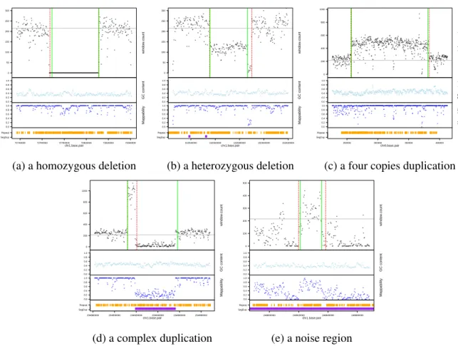
for modeling of copy number. In contrast, existing methods find only two general types of copy numbers, i.e. loss/deletion and gain/duplication. The support for the seven state modeling strategy is evident from examples shown in Figure 2.2, where GENSENG correctly recovered high-confidence CNVs and identified their status as homozygous deletion (Figure 2.2 (a)), heterozygous deletion (Figure 2.2 (b)), and multi-allelic duplications (Figure 2.2 (c)-2.2 (e)). Each subfigure 2.2 (a)-2.2 (e) has 4 panels from top to bottom, and the X-axis of each subfigure indicates genomic position in base pairs. In the first panel, the black dots on the Y-axis indicate read-depth signal; red dashed lines are boundaries from GENSENG prediction; green solid lines are boundaries reported in the high-confidence CNV set (Mills et al., 2011); grey lines are the median read-depth of the
number 4 from a noisy region with a median mappability of 0.58, illustrating good sensitivity for detecting duplications by employing simultaneous bias correction and copy number inference.Some discrepancies in the boundaries between the predicted CNVs and the high-confidence CNVs were observed, reflecting technological differences between HTS and microarrays.
● ● ● ● ● ● ● ● ● ● ● ● ● ● ●● ● ●● ● ● ● ● ● ● ● ● ●●● ● ● ● ● ●●● ● ● ● ● ● ● ● ● ● ● ● ● ● ●● ●● ● ● ● ● ●● ● ● ●● ● ● ● ●●● ● ● ● ● ● ● ● ● ● ● ● ● ●● ●● ● ● ● ●● ● ● ●● ● ● ● ● ●●●●●●●●●●●●●●●●●●●●●●●●●●●●●●●●●●●●●●●●●●●●●●●●●●●●●●●●●●●●●●●●●●●●●●●●●●●●●●●●●●●●●●●●●●●●●●●●●●●●●●●●●●●●●●●●●●●●●●●●●●●●●●●●●●●●●●●●●●●●●●●●●●●●●● ● ● ● ● ● ● ● ● ● ● ● ● ● ● ● ● ● ● ● ● ● ● ● ● ● ● ● ● ● ● ● ● ● ● ● ● ● ● ● ●● ● ●● ● ● ● ● ● ● ● ● ● ● ● ●●● ● ● ● ●● ● ● ● ● ● ●● ● ● ● ●●●● ● ● ● ●● ● ●● ● ● ● ● ● ●● ● ● ● ● ● ● ● ● windo w.count 0 50 100 150 200 250 300 ● ●● ●● ●●●● ●●●● ●● ● ● ● ● ● ● ●●●●●●●●●●● ●●●● ●● ●● ●●● ●● ●●● ●● ● ● ● ●●●●●●●●●●● ●●●●●●●●● ●● ● ● ●● ●●●●●●●●●● ● ●●● ● ●● ●●●● ●●●●● ● ● ● ●●● ●● ●●●●●●●●●●●●●●● ●● ●● ●● ●●●● ●●● ●●●●●●●●●●●●●●●● ●●●●●●●●●●●● ● ●● ● ●●● ●● ●●●●●●●●●●● ●●●●●● ●● ●●●●●●●●●●●● ●● ●● ●●● ● ●●●●●● ● ●●● ●●●●●●●●●●●●●●●●●● ● ●●●● ●●● ●●● ●● ●●●●●● ●● ●●●● ●●●●● ●●● ●● ●● ●●●● ●● ● ●●● ●●● ● ● ●●● ●●●● ●●●●●●●●●●●●●●● ●● ●●●●●●● ●● ● ●●● ● ● ● ● ● ●● ●● ●● ● ●●● GC content 0.0 0.2 0.4 0.6 0.8 1.0 ●● ● ●●●●●● ● ● ●● ●●●●●●●●●●●●●●●●●●●●●●●●●●●●●●●●●●●●● ● ● ●●●● ● ● ●●●●●●●●●●●●●●●●● ● ● ●●●●●●●●●●● ● ●● ●● ● ● ● ● ●●●● ●● ●● ● ● ●●● ● ● ●●●●●●●●●●●●●●●●●●●● ●● ●●● ● ●● ●●● ● ● ●● ●● ●●●●●●●● ● ● ● ●●●● ●●●●●●●●●●●● ● ● ●●●●● ● ●● ● ●●●●●●●●●●●●●●●●●●●●●●●● ● ● ●●●●● ● ●● ● ● ● ●● ● ● ●● ●●●●●●●●●●●●●● ●● ●●●●●●●●● ● ● ● ●●●●●●●●●●●●●●● ● ● ● ●● ●● ●●●●●●●●●●●●●●● ● ● ●●●●●●●●●●●●●●●●●●●●●●●●●●●●●●●●●● ● ● ● ●●● ● ● ●●● ● ● ● ● ● ●● Mappability 0.0 0.2 0.4 0.6 0.8 1.0
72740000 72760000 72780000 72800000 72820000 72840000 SegDup
Repeat
chr1.base.pair
(a) a homozygous deletion
● ● ● ● ● ● ● ● ●● ● ● ●● ● ● ● ● ● ● ● ●● ● ● ●●● ●● ● ● ●●● ● ●● ● ● ● ● ● ● ● ● ●● ● ● ● ● ● ● ●● ● ● ●● ● ● ● ● ●● ● ● ● ● ● ● ● ● ● ● ● ● ● ●●● ● ● ● ● ● ● ● ● ● ●●● ● ● ● ● ● ● ● ● ● ● ●●● ● ●● ●●● ● ●● ● ●● ● ●● ● ● ● ● ● ● ●● ● ● ●● ● ● ● ● ● ● ● ● ●● ● ● ● ● ●●● ● ● ● ●● ● ● ● ● ● ●●●●● ● ● ● ● ● ● ●●●● ●●● ● ● ●● ●● ● ● ● ● ● ● ● ● ● ● ● ● ● ●● ●●● ● ● ● ● ●●●● ● ● ● ● ● ● ● ● ● ● ● ●●● ● ● ● ● ● ● ● ● ● ● ● ● ● ● ●● ● ● ● ● ● ●● ● ● ● ● ● ● ● ● ● ● ● ●● ● ● ● ● ● ● ● ●● ●● ● ● ● ● ● ● ● ● ● ● ● ● ● ● ● ●● ● ● ● ● ●● ● ● ● ● ● ● ● ● ● ● ● ● ● ● ● ● ● ● ● ● ● ● windo w.count 0 50 100 150 200 250 300 ● ●● ● ●● ●●●●●●●● ●●●● ●●●●● ●●●● ●● ●●●●● ● ●●●●● ●● ● ●● ●● ● ●●●●●●●●● ●●●●● ●●● ●● ●●●●● ●●●●●●●●● ● ●●●● ●●● ●● ●● ●● ● ●●●● ●●●●● ● ● ●●● ● ●●●●●●●●●●●●●●●●●●●●● ● ●●●● ●●●●●●●●●● ●●●● ● ●●●●● ● ●●●●●● ●● ●● ● ●● ●●● ●●●●●●●● ●●●●●●●●● ●●●●●●● ● ● ● ●●●● ●●●●●●●●●●●●●●● ●● ●●●●●●●●●●● ●●●● ●● ● ● ●●● ●● ●●●●●●●● ●● ●●●●● ●●●●●●●●●● ●● ●●●●● ● ● ● ●●●●●●●●●●●●● ●●● ●● ●●●●● ● ● ● ● ●● ●●●●●●● GC content 0.0 0.2 0.4 0.6 0.8 1.0 ● ● ● ● ● ● ●●●●●●●●●●●●●●●●●●●●●●●●●●●●●●●● ● ● ●●● ● ● ●●●●●●●●●●●●●●●● ● ● ●●●●●●●●●● ● ● ● ● ● ● ●●●●●● ●● ●● ●● ●●● ● ● ●●●●●●●●●●●●●●●●●●●●● ●●●●●● ● ● ● ● ●●●●● ● ● ●●●●●●●●●●●● ● ● ●●●●●●●●●●●●●●●●●●●●● ● ● ● ●●●●●●●●●●●●●●●●●●●●● ● ● ●●●●●●●●●● ● ● ● ●●● ●● ● ● ● ● ●●● ●● ●●● ● ● ●●● ● ●●●●●●●●●● ● ● ●●●●●●●●●●●●●● ●● ●● ●● ● ●● ● ● ● ●● ●● ●● ● ● ● ●● ●●●●●●●●●●●●●●●● ● ● ● ●●●●● ● ●●●●●●●●●●●● Mappability 0.0 0.2 0.4 0.6 0.8 1.0
152540000 152560000 152580000 152600000 152620000 SegDup
Repeat
chr1.base.pair
(b) a heterozygous deletion
● ●●●●●● ●● ●●●●●● ● ● ● ● ● ● ● ● ● ● ● ● ● ● ● ● ●● ● ● ● ● ●● ●● ● ● ● ● ●● ● ● ● ●●● ●● ● ● ●● ● ● ● ● ● ● ● ●● ● ● ●● ● ● ● ● ● ● ● ●● ●● ● ● ●● ● ● ● ● ● ● ● ● ● ●●●● ● ● ● ● ● ● ● ● ●● ●● ●● ● ●● ● ● ● ● ● ●● ● ●● ● ● ● ● ●●●● ● ● ● ● ● ● ● ● ●●● ● ● ● ● ●● ● ● ● ● ● ● ● ● ● ● ● ● ● ● ● ● ● ● ● ● ● ● ● ● ● ● ● ● ● ● ●● ● ● ●● ● ●●● ● ● ● ●● ● ● ● ● ● ● ●● ● ● ● ● ●● ●● ●● ● ●● ● ● ● ● ● ●● ●● ● ● ● ● ● ● ●● ●● ● ● ●● ● ●● ● ● ● ● ●●● ● ●● ● ●● ● ● ●● ●●●●●● ● ● ●● ● ● ●● ● ●● ● ● ● ●● ● ● ●● ● ● ● ● ● ● ● ●●● ● ● ● ● ● ● ●●● ● ● ●● ●● ●● ●● ●● ● ● ● ● ● ●●● ●● ● ● ● ● ● ● ● ● ●● ● ●● ●● ● ● ● ● ● ● ●● ● ● ● ● ● ● ● ● ● ●● ● ●● ● ●● ●●● ● ● ● ● ●● ●●● ● ● ● ● ● ● ● ● ● ● ● ●● ● ●● ● ● ● ● ● ● ●●● ● ● ● ● ● ● ● ● ● ●●● ● ● ● ●● ● ● ● ● ● ● ● ● ● ● ● ● ● ●●● ● ● ● ● ● ● ● ● ● ● ●●● ●●● ●● ● ● ●● ● ● ● ● ● ● ● ●● ● ● ● ● ● ● ● ● ●●●●● ● ●● ● ● ● ● ●● ●● ● ● ● ● ● ● ● ● ● ●● ● ● ● ● ● ● ● ●● ● ● ● ● ●● ● ● ●● ● ● ● ●●●● ●● ● ● ●● ●● ●● ●●●●● ● ● ● ● ● ● ● ●●● ●●● ● ● ● ● ● ●● ● ● ● ● ● ● ● ● ● ●● ● ●● ●● ●●●●●● ● ● ● ● ●●● ●●●●● ● ● ● ● ● ● ● ●●●●●●●● ●●●● ● ●●●● windo w.count 0 200 400 600 800 1000 ●●●●●●●● ● ●● ● ●●● ●● ●● ●●●●● ●● ●●●●●●●●●● ● ●●● ● ● ●●●●●●● ●● ●●●●●●●●●●●●●●●● ●● ●●● ● ● ●● ● ● ●● ●● ● ●●●●●●●● ● ●●●●●● ● ● ● ● ● ●●●●●●●● ●●●●●●●● ●●●●●● ●●● ●●● ●●●● ●●●●●●● ●●●●●● ●● ●●●●●●●● ●● ● ●●●●●●● ● ● ● ●●●● ●●●● ● ●● ●● ● ●●●● ● ●●●●●●●●●● ●● ● ●●●●●●●●●● ● ●●●● ● ● ● ● ●● ● ●●●●● ●●●●● ● ●● ●●●●● ● ●●●●●● ●●● ●●●●●● ●● ●●●●● ●● ●●●●●● ●● ●●● ● ● ●● ●●●● ● ● ● ● ● ●●●●●●●●● ● ● ●●●●● ●●●● ●●●●● ●●● ●●●●●● ●●●●●●●● ●● ●●● ●●●●●●●● ●●●● ●●●●● ● ●● ● ●●● ●● ●●●●●●●● ●●● ●●● ●●● ●●●●●●●●● ●● ●●●● ●● ●●●●●● ●●●●●●● ●●●● ●●● ●●● ●●● ●●●● ●●●●●● ●●●●●●●●●● ● ●● ● ● ● ●●●●●●●●●●●●●●●● ●● ●●● ●●●● ● ● ●●●●●●●●●●●● ●●●● ●● ●● ●●● ● ● ●●● ●● ●● ●●●●●● ● ● ● ●●●●●●●●●● ●● ● ●● ●● ●●●●● ● ● ●●●●● ●● ●●●●●●●● ● ● ● ●● ●● ● ● ●●● ●●●● ●● ● ● ●● ● ● ● ●● ●●●● ●● ●●●●●● ●● ● ● ●●● ●●●●● ●● ●●●●● ●● ●●●●● GC content 0.0 0.2 0.4 0.6 0.8 1.0 ●●●●●●● ● ● ● ●●●● ● ● ● ● ● ● ● ●●● ● ● ● ● ● ● ● ● ●●●●● ● ● ●● ●● ●●●●● ● ● ●●● ● ● ● ● ●● ● ● ●● ●●●● ● ● ● ● ● ● ● ● ● ●● ●● ●● ● ● ● ●●●●● ●● ●● ●● ●●●● ● ● ●●●●● ●● ●●●●●●●● ● ● ● ●●●● ● ●● ● ●●●●●●● ● ● ● ● ● ● ●●●●●●● ● ● ●●●●●●●●● ● ●●●●●●●● ●● ●●●●●●●● ● ● ● ●●●● ●● ●●●●●●●●●●● ● ● ● ●●●●●●●●●● ● ● ●●●●●●●●●●●●●●●●● ● ● ●●●●●●●●●●●●●●●●●●●●●●●●●●●●●●●●●●●●●●●●●●●●●● ●● ●●● ● ● ●●●●●●●●●●●●●●●●●●●●●●●●●●●●●●●●●●●●●●●●●●● ● ● ●● ● ● ● ●●●●●●●● ● ● ●●●●●●●●●●●●●●●●●●●●●●●●●●●●●●●●●●●●●●●●● ● ● ● ●● ●●●●● ● ● ●●●●●●●●●●●●●●●●●●●●●●●●●●●●●● ●● ●●● ●● ●●●●●●●●●●●●●●●●●●●●●●●●●●●● ● ● ●●●●●●●●● ●● ●●●●●● ● ● ● ● ● ● ●●● ● ● ●● ● ● ● ● ●●●●● ●● ●●●●●●●●●●●●●●●●●●●●●●●●●●●●●●●●●●●●●●●●● ● ● ●●●●●●●●●●●●●●●●●● ● ● ● ●●●●●●●●●●●●●●●●● ● ● ● ●●●●●●●●● ● ● ●●● ● ●●●●●●●●●●●●●●●●●● Mappability 0.0 0.2 0.4 0.6 0.8 1.0
250000 300000 350000 400000 SegDup
Repeat
chr6.base.pair
(c) a four copies duplication
●● ●●●●● ●●●● ● ●●● ●●● ●●● ● ● ●●●●● ●● ●●●●●● ●● ● ● ● ● ● ● ●●● ●●●● ●● ●● ● ● ● ● ● ● ● ● ● ● ●● ● ● ● ●● ●●● ●●●●● ● ● ● ●●●● ● ● ● ●● ● ● ● ●● ● ●● ● ● ● ● ● ● ● ● ● ● ● ● ● ● ● ● ● ● ●● ● ● ● ● ● ● ●● ● ●● ●● ●● ● ●● ●● ●●●●●●●●●●●●●●●●●●●●●●●● ●●●● ●● ●●●●●●● ●●● ● ● ●●● ● ● ●● ● ● ●●● ● ●● ●● ●●●●●●● ● ●●● ●● ●● ●●●●●●●● ●●●●●●● ●●●●●●●●● ● ● ●●●●●●● ● ● ● ●●●●●● ● ● ●● ● ●● ● ● ●● ●● ●● ● ●● ●●●●● ●● ● ●●● ● ● ● ●●●●●● ● ● ● ● ● ●●● ●●●● ● ● ● ●●● ● ● ●●●● ● ● ●●●● ● ● ● ● ●● ● ● ● ●● ● ●● ● ● ●●●●● ●● ●● ● ● ● ● ● ●● windo w.count 0 200 400 600 800 1000 ●●● ● ● ●● ●●●●●●●●●●●●●●●●● ●●●● ●● ● ●● ●● ●●● ●● ●●●●●●●●●●●●●●●●●●●●●●●●●●●●●●●●●●●●●●●●●●● ●●●●●●●● ● ● ●●●● ●● ●●● ●●●●●●●●●●● ●● ●● ●●●●●●●●●●●●●●●●●● ●● ●●●● ●● ● ●●●● ●● ●● ● ●●● ●●●●●●●●●●●●● ●●●●●●●●●●●● ●●●●●●●●● ●●●●●●●●●●●●●●●● ●●●●●●●●●●●●●●●●●● ●●● ●● ●● ●●● ●●● ●●● ● ●●●●●●●●●● ● ●●●●●●●●●●●●●●●●●●●●●● ●● ● ●● ●●● ●● ● ● ● ●●●●●●●●● ●● ●●●●●●●●● ●● ● ● ● ● ●●● ● ●●● ●● ●● ●●● ●●● ● ●●●●●●●●●●●●●●●●●●●●● ●●● ● GC content 0.0 0.2 0.4 0.6 0.8 1.0 ●●●●●●●●●● ● ● ●● ●●●●●●●●●●●●●●●●●●●●●●●●● ● ● ●●●●●●●●●●●● ● ● ● ● ● ●●●● ● ● ● ●● ● ● ●●●●●●●●●●●●●●●●●●●●● ● ● ●●●●●●●●●●●●● ●● ●●●●● ● ● ●●●●●●●●●● ● ● ● ●● ● ● ● ● ● ● ● ●● ● ● ● ● ● ●● ●●● ● ● ● ● ● ● ● ● ● ●● ● ●●●● ●● ● ● ●● ●● ● ● ● ● ● ● ●● ● ● ●● ● ● ● ● ● ● ● ●● ● ● ● ● ●● ●●●●●●●● ●●● ● ● ● ● ● ● ● ● ●●● ● ● ● ● ● ● ● ● ● ● ● ● ● ● ●● ●●● ● ● ●●●● ●● ● ●●●●●●● ● ● ●●● ● ● ●● ●●●●●●●●●●●●●●●●●●● ●● ●●●●●●●●● ● ●●●●●●●●●● ●● ●●●● ● ● ●●●●●●●●●●● ● ● ●●●●●●● ● ● ● ● ● ●●●●●●●● ● ● ● ● ●●●●● Mappability 0.0 0.2 0.4 0.6 0.8 1.0
234880000 234900000 234920000 234940000 234960000 234980000 SegDup
Repeat
chr1.base.pair
(d) a complex duplication
● ● ● ● ● ●● ● ● ● ●● ● ● ●● ● ●● ● ● ● ● ● ● ●● ●● ● ● ● ● ● ● ● ●● ● ● ● ● ● ● ● ●● ● ● ● ● ● ● ● ● ● ● ● ● ●●● ● ● ● ● ● ● ● ● ● ● ● ●●● ● ● ● ●● ●●●●●● ● ●●● ● ●●● ● ●●●●●● ● ● ● ● ● ● ● ● ● ● ● ● ● ● ● ● ● ● ● ● ● ●● ● ● ●● ● ● ● ● ● ● ● ● ●● ●●● ● ● ● ● ● ● ● ● ● ● ● ● ●● ● ● ● ● ●● ● ● ●● ● ● ● ● ●●● ● ● ● ● ● ●● ● ●● ● ● ● ● ● ● ● ● ●● ●●● ● ● ● ● ●●●● ● ●● ● ●●●●●●●●●● ● ●● ●● ●●●●● ● ● ● ●● ●●●● ● ● ● ● ●●● ●●● ● ● ● ●● ●●●●● ●● ●●●● windo w.count 0 100 200 300 400 500 ●●●●●●● ● ● ●●● ●● ●●● ●●●●● ●●● ● ● ●●●●●●●●●●●●●●●●●●●●●● ● ●● ● ●●●●●●●●●●●● ● ●● ● ●●●●●●●●● ●● ●●● ● ● ●●● ●●●●●● ●●●●●● ●● ●●●●●● ●●● ●●●●●●●●●●●●●●●●●● ● ●●●●●●●●●●●●● ●● ●●●●●●●●●●● ● ●●● ● ●●●●●●●●●●●●● ●● ● ● ●● ● ● ● ● ●● ● ●● ●●● ● ● ●●●●●●●●● ●● ● ● ● ●● ●●●● ● ●●●●● ●● ●●●●●●●● ●● ● ● ●● ●●●●●●●● ●● ● ● ● ●●●●●●●●● ●●●●● GC content 0.0 0.2 0.4 0.6 0.8 1.0 ● ● ● ● ● ● ● ● ● ● ●● ● ● ● ● ● ● ●● ●● ● ● ●● ● ● ● ● ● ● ●● ● ● ●● ● ●● ●● ● ● ● ● ●●● ● ● ●● ● ● ● ● ●●● ● ● ● ● ●● ●● ●●● ● ● ● ● ● ● ● ●● ● ●●●● ● ●●●●● ●●● ● ● ●● ●●● ● ● ● ● ●● ● ●● ● ● ● ●●● ● ● ● ● ● ●● ● ●● ● ●●● ● ● ●● ● ● ●● ●● ● ● ● ● ● ● ● ● ●● ● ●● ●● ● ● ● ● ●● ● ● ●● ● ● ●● ● ● ● ● ● ● ● ● ● ● ●● ● ●● ● ● ● ● ● ● ●● ● ● ● ●●● ● ●●●●● ● ● ● ●●●●● ● ●●●●● ● ● ● ● ●● ●● ● ● ● ● ●● ●●● ● ● ● ● ● ●●● ● ●● ● ● ●●● ●●●● ● ●● ●●● ● Mappability 0.0 0.2 0.4 0.6 0.8 1.0
248600000 248620000 248640000 248660000 SegDup
Repeat
chr1.base.pair
(e) a noise region
Figure 2.2: Example high-confidence CNVs predicted by GENSENG: NA12878 HTS
sensitivity for detecting duplication from a noisy region with a medium mappability score (0.58) after accounting for mappability and additional noises.
Multiple techniques were introduced in GENSENG, including correcting for GC content and mappability, modeling autoregression, fitting a mixture of negative binomial and uniform distributions, and applying quality control to prioritize CNV calls (Methods). To study the effects of these techniques on CNV detection and identify the best-fitting model, we examined the sensitivity and the number of CNV calls made by different partial versions of our method (Table 2.3). We found that correcting for GC content alone was not sufficient; and further correcting for mappability resulted in the most substantial improvement, with gains in both sensitivity and specificity. Quality control including both size and RDA filters substantially improved specificity with minimal loss in sensitivity. The best GENSENG model was selected based on these results and included all aforementioned techniques.
2.2.4 CNV detection method
This triplet of data for each individual genome is input into an integrative hidden Markov model (HMM), which classifies each window to a copy-number state based on maximum a posteriori probability, while simultaneously accounting for sources of bias. The state changes mark the predicted breakpoints of CNVs. Below we present our method and the elements needed in HMM characterization.
Hidden states and transition probability. While microarray analysis suffers from
oversaturation at high copy numbers, HTS allows RD-based methods to determine high copy numbers with improved accuracy (Campbell et al., 2008). The state represents the underlying copy number (CN). The state variableqt =CNtis hidden and discrete withN possible values,
(0,1, ..., N −1). The total number of hidden statesN is implemented as an input parameter of
can be derived from the data by K-mean clustering the logarithm of the read-depth.For the HTS datasets used in this study, we assume seven hidden states representing copy numbers of 0, 1, 2, 3, 4, 5, and 6 or more. For homozygous populations such as inbred mice, we assume four hidden states representing copy numbers of 0, 2, 4, and 6 or more. We collapse the duplications with 6 or more copies into one state, because they are difficult to distinguish because of both experimental (reduced signal-to-noise ratio) and computational concerns (having few regions with very high read-depth signal). State transitions proceed from one window to the next according to a first-order time-homogeneous Markov process. The transition probability describes the probability of having a copy-number state change between two adjacent windows. Letπj be the initial state probability, the probability that the state of the first window is statej. The underlying hidden Markov chain is defined by state transitionsP(qt|qt−1)and is represented by a time-independent stochastic
transition matrixA={ajz}=P(qt=z|qt−1 =j). Intuitively, the copy number state is unlikely to
change for nearby windows but is more likely to change for windows that are far apart.
Emission probability. The hidden copy-number states emit probabilistic outputs at each
window, i.e. the observed RD signal representing integer-valued count data. In the absence of sources of bias, sequencing coverage is uniform across the genome such that the emission
probability of RD could be modeled by a Poisson distribution with equal mean and variance. In the presence of sources of bias, sequencing coverage is not uniform and the Poisson-distribution assumption fails. To account for biases, the emission probability of RD is modeled as a mixture of uniform distribution and negative binomial (NB), expressed as the following:
e(t, j) = P(Ot=ot|qt=j) = c/Rm+ (1−c)eN B(t, j)
= c
Rm
+ (1−c)Γ(ot+ 1/(φj))
ot!Γ(1/φj)
( 1
1 +φjµtj
)1/φj( φjµtj
1 +φjµtj
)ot,
the state variable,otis the RD signal for windowt,µtj is the mean RD for windowtgiven statej,
φj is the overdispersion parameter given statej. To describe the negative binomially distributed component,eN B(t, j), we first explain the relationship between the Poisson and the negative binomial distributions. The Poisson distribution imposes that the variance equals to the mean. The negative binomial distribution allows overdispersion. Specifically, ifO follows a Poisson
distribution with meanµ, andµfollows a gamma distribution, the resulting distribution forO is a negative binomial distribution. The variance of negative binomial distribution isµt+φµ2t, where
φµ2t is the overdispersion part of the variance. Asφ→0,fN B(ot;µt, φ)reduces to a Poisson distribution with meanµtand varianceµt. fP(ot;µt) =
exp(−µt)µott
ot! . Next, the mean value of the
negative binomially distributed component is expressed as a function of a set of covariates to account for confounders.
µtj = α0∗(CNt)β1 ∗(lt)β2 ∗(gt)β3 (2.1)
wheretdenotes thetth window,j is the index of the copy number state,j emphasizes the dependency of the meanµton the copy numberCNt,ltis the mappability score,gtis the GC content. For computational convenience, we setCNt = 0.5whenj = 0, and setCNt=j when
j >0.
We then employ a log link function to acknowledge the fact thatµtj >0and obtain:
log(µtj) = β0+β1∗log(CNt) +β2∗log(lt) +β3∗log(gt) (2.2)
β0, β1, β2, β3are the regression coefficients. Specifically,β0 = log(α0), is the intercept parameter
and is interpreted as the average level of read-depth signal when all covariates are equal to zero. β1
is the amount of increase of read-depth for every unit increase of copy number, CN.β2 is the
amount of increase of read-depth for every unit increase of the mappability score,l. β3 is the
The uniform distribution has a density function1/Rm to model any random fluctuation of read depth, whereRmis treated as a known constant using the largest RD among all windows of the chromosome. When non-overlapping windows are used, the mean RD for each window,µtj, is modeled by a negative binomial regression model, where the predictors include copy-number state, GC content, and mappability score. A standard HMM assumes the Markov property,
P(qt|qt−1, qt−2, qt−3, ...q1) =P(qt|qt−1). An additional assumption that is often employed is that
the observations are independent given the states,Ot⊥Oi(i6=t)|qt, which is valid when the windows are non-overlapping. When the windows are overlapping, this assumption is invalid; and instead, the observations are drawn from an autoregression process (Juang and Rabiner, 1985). We have implemented an autoregressive HMM to model this feature of the data. Specifically, a residual term is included as an additional predictor in the negative binomial regression model assuming first order autoregression. Thus in each round of inference, we would first fit the model and obtain the expected read count of statej at windowt µt−1,j, and calculate residual
rt−1,j = log(ot−1)−log(µt−1,j)fort >1and letr1,j = 0. With this extra predictor, we will run
GLM again to obtain the true expected read count of statejat windowt µt,j. The additional noise in the data that cannot be explained by variability in GC content and mappability are
accommodated by,φj, the overdispersion parameter of the NB distribution (allowing variance to be larger than mean) and the uniform distribution in the mixture model.
Tuning parameters. Given the HMM topology, the challenge lies in optimizing model
Parameter estimation. The optimization problem is solved by the Baum-Welch algorithm (Baum et al., 1970), which maximizes the data likelihood for an individual chromosome in iterative steps including initialization, expectation, and maximization. Following Bilmes (Bilmes, 1998), we define the complete-date likelihood and solve theQfunction in order to find the maximum
likelihood estimates (MLE) of the HMM parameters. In the initialization step, we rely on intuitive guesses as well as empirical values. The initial emission parameters were estimated from the 1000GP and the Mouse Genomes Project datasets where known CNVs are available. These initial emission parameters are saved for the human and mouse genomes respectively and are used for any new sample without prior knowledge of its CNVs. In the maximization step, we obtain
maximum-likelihood estimates of emission parameters. Because we fixcandRm as constant, parameter estimation will only concern the negative binomially distributed component. We apply a weighted negative binomial regression model, where the weights are posterior probabilities for each window belonging to a particular copy-number state, given the observed data of an entire
chromosome. These weights represent current knowledge of the probabilistic classification of a window to copy-number state and are updated in the expectation step. While included as a predictor in the regression model, the copy number is the hidden variable to be inferred from the observed data. Intuitively, by using posterior probability as regression weights, we are able to partition the observed RD across all hidden states, proportional to the likelihood. The weighted NB regression model is fitted by alternately estimating regression coefficients using iteratively reweighted least squares and estimating the overdispersion parameter using a Newton-Raphson method. In the expectation step, we update the forward, backward, and posterior probability given the current estimates from the maximization step. The expectation and maximization steps iterate until the convergence criterion (smaller than10−6 change in the log-likelihood) is reached.
CNV calling. Using the parameters at convergence, first we obtain the final estimates of the
breakpoints of CNVs. The confidence score of a CNV region is computed as the sum of the posterior probabilities of all windows enclosed within the breakpoints. Next, a two-step merging algorithm is carried out to refine the boundaries of the CNVs.
Prioritization of CNV calls. A CNV quality control step can be applied to remove CNVs
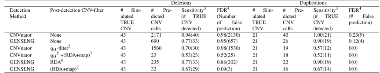
predicted with the lowest confidence. We recommend removing predicted CNVs shorter than 800bps (i.e. removing those that appear in only one window as shown in Table 2.3), or predicted CNVs with an average mappability lower than 0.3 (i.e. removing those that cannot be confidently predicted as shown in Figure 2.6 (b)). An additional prioritization approach was implemented via the read-depth-accessibility (RDA) statistic, which reflects the signal-to-noise ratio of a predicted CNV region after accounting for known confounders in read-depth. The term of
read-depth-accessibility was first coined by Abyzov et al. (Abyzov et al., 2011), but for a different purpose. The RDA statistic is computed in 3 steps: (1) after CNV calling, identify all compatible copy-number-neutral windows whose GC-content and mappability scores are the same as those from the region of interest; (2) calculate the average window counts from (1) as the expected read-depth for the region of interest; (3) obtain the RDA by dividing the observed read-depth by the expected read-depth for the region of interest. Using a copy number of two as normalization for copy-number-neutral autosomal regions, the theoretical signal-to-noise ratios are 0, 0.5, 1.5, and 2 for copy numbers of 0, 1, 3, and 4, respectively. Therefore, a region is considered to be
read-depth-accessible if its RDA value is lower than 0.5 for homozygous deletions, lower than 0.75 for heterozygous deletions, and greater than 1.25 for duplications. In general, we recommend removing CNVs predicted from regions that are not read-depth-accessible (e.g. if its RDA values range between 0.75 to 1.25). In addition, we recommend ranking the predicted regions by their RDAs, where a higher signal-to-noise ratio reflects higher confidence that the predicted CNVs are correct; this is analogous to ranking by fold-change in gene-expression analysis.
2.2.5 Performance assessment
Therefore, we used two approaches to assess our methods performance. First we conducted a simulation to estimate the sensitivity and specificity to detect CNVs. Then we analyzed the high-coverage 1000GP trio data, where we estimated the sensitivity using high-confidence CNVs and used the total number of base pairs or calls as a surrogate measure for specificity. For
comparison, we applied CNVnator (Abyzov et al., 2011) in parallel, using its recommended parameter setup and QC filter. The methodology differences between GENSENG and CNVnator are detailed in Table 3.2. The main differences are in bias correction and segmentation techniques.
Simulation. We simulated two datasets for performance assessment. The first simulation
directly generated read-depth data (Yoon et al., 2009). Using chromosome 1 from NA12878 as a template, we implanted 76 high-confidence CNVs (25 duplications and 51 deletions) (1) by assigning a copy number of four to any window that overlapped the duplications and a copy number of zero to any window that overlapped the deletions. All other windows were assigned to have a copy number of two. The covariate matrix (the assigned copy number, mappability score, and GC content of each sliding window) and coefficient vector were passed to the garsim function from R/gsarima to simulate the read-depth for each window. The garsim model we applied was the negative binomial distribution with the log link function, where the autoregressive parameter was set to 0.6, the zero correction parameter was set to zq1, and the inverse of the overdispersion parameter was set to 0.01.
The second simulation mimicked a sequencing experiment to generate paired-end reads from a CNV containing a hypothetical chromosome. To simulate reads, we used chromosome 1 of the reference human genome as a template and modified the template sequence based on the 76 high-confidence CNVs (51 deletions and 25 duplications) (Mills et al., 2011). For any deletion, we removed the corresponding sequence of the deleted DNA, and for any duplication, we inserted an extra copy of the duplicated sequence. As a result, the implanted deletions were copy number 0 deletions, and the implanted duplications were copy number 4 duplications. Among the 76
chromosome 1. Second, after the CNV-containing hypothetical chromosome was created, we applied the sequencing simulator, wgsim, as implemented in SAMTools (Li et al., 2009) to generate 36bp paired-end short reads. For wgsim simulation, the mean value of the outer distance between the two ends was set to 200, the standard deviation was set to 20, and the sequencing error model was the empirical error model of the Illumina sequencing platform. A total of 150 million
paired-end reads were generated, which gave an average sequencing coverage of 40x. Third, we used BWA (Li and Durbin, 2009) to map the reads to the unmodified reference human genome. The resulting alignment file was use as input to apply GENSENG (Szatkiewicz et al., 2013) and CNVnator (Abyzov et al., 2011). Among CNVs predicted by either approach, a true discovery was defined when a predicted CNV overlapped with at least 50% of a simulated CNV and had the same copy number.
1000GP data. We analyzed the high-coverage sequencing data for the CEU trio from the
1000GP. To facilitate the comparison between the predicted CNVs and the high-confidence CNVs, which only provide deletion and amplification calls rather than the particular copy number, we defined deletions as any GENSENG calls where the inferred copy numbers were 0 or 1, and duplications as any calls where the inferred copy numbers were greater than 2. Sensitivity was calculated by dividing the number of total base pairs of the overlapping events (>1bp overlap, or
>50% reciprocal overlap with the high-confidence CNVs) by the total number of high-confidence CNVs.
Performance on low coverage data: The native coverage of both our simulated data and the
1000GP high-coverage data is∼40x. To identify the lower bound that GENSENG can handle, we applied GENSENG to data with varying sequencing coverage and compared the performance to that based on the native coverage using the same evaluation metrics. First, we repeated the