Multi-view dynamic scene modeling

(1)

Multi-view Dynamic Scene Modeling

Li Guan

A dissertation submitted to the faculty of the University of North Carolina at Chapel Hill in partial fulﬁllment of the requirements for the degree of Doctor of Philosophy in the Department of Computer Science.

Chapel Hill 2010

Approved by:

Marc Pollefeys, Advisor

Jean-S´ebastien Franco, Co-principal Reader

Leonard McMillan, Reader

Jan-Michael Frahm, Reader

(2)

c ⃝2010 Li Guan

(3)

Abstract

Li Guan: Multi-view Dynamic Scene Modeling. (Under the direction of Marc Pollefeys.)

Modeling dynamic scenes/events from multiple ﬁxed-location vision sensors, such as video

camcorders, infrared cameras, Time-of-Flight sensors etc, is of broad interest in computer

vision, with many applications including 3D TV, virtual reality, medical surgery,

marker-less motion capture, video games, and security surveillance. However, most of the existing

multi-view systems are set up in strictly controlled indoor environments, with ﬁxed lighting

conditions and simple background views. Many complications limit the technology in the

nat-ural outdoor environments. These include varying sunlight, shadows, reﬂections, background

motion and visual occlusion etc. In this thesis, I address diﬀerent approaches overcoming all

of the aforementioned diﬃculties, so as to reduce human preparation and manipulation, and

to make a robust outdoor system as automatic as possible.

The main novel technical contributions of this thesis are as follows: a generic heterogeneous

sensor fusion framework for robust 3D shape estimation; a way to automatically recover 3D

shapes of static occluder from dynamic object silhouette cues, which explicitly models the static

“visual occluding event” along the viewing rays; a system to model multiple dynamic objects

shapes and track their identities simultaneously, which explicitly models the “inter-occluding

event” between dynamic objects; and a scheme to recover an object’s dense 3D motion ﬂow over

time, without assuming any prior knowledge of the underlying structure of the dynamic object

being modeled, which helps to enforce temporal consistency of natural motions and initializes

more advanced shape learning and motion analysis. A uniﬁed automatic calibration algorithm

for the heterogeneous network of conventional cameras/camcorders and new Time-of-Flight

(4)

To my parents

for letting me pursue my dream for so long

so far away from home &

To my wife

(5)

Acknowledgments

I would like to thank my advisor, Marc Pollefeys, for supporting me over the years, and for giving me so much freedom to explore and discover new areas of dynamic scene modeling. My other committee members have also been very supportive. Jean-Sébastien Franco has long been an inspiration to me. His precise suggestions and thorough discus-sions with me are one of my best learning experiences at Chapel Hill. Leonard McMillan brings in-depth experience to my thesis, as a well-known researcher with great contri-butions in related areas throughout the years. Jan-Michael Frahm proves to be a most considerate mentor and friend who is always supportive with all projects that I partici-pate. Svetlana Lazebnik always give me suggestions right to the point and show me the ray of hope through the darkness of desperations. Also special thanks are to Edmond Boyer who has always been inspiring and generously shared his brilliant ideas with me. I would like to thank my many friends and colleagues at UNC-Chapel Hill and at ETH-Zürich with whom I have had the pleasure of working over the years. These include Sudipta Sinha, Seon Joo Kim, Christopher Zach, Changchang Wu, David Gallup, Brian Clipp, Megha Pandy, Roland Angst, Friedrich Fraundorfer, Gabriel Brostow and all the members of the Computer Vision Group at UNC-Chapel Hill and Computer Vision and Geometry Lab at ETH-Zürich.

(6)

List of Figures

1.1 Multi-camera network setup. . . 2

2.1 Checkerboard camera network calibration. . . 8

2.2 Foreground silhouette and visual hull formation. . . 11

2.3 Visual hull of a concave shape. . . 12

2.4 Triangulation of 3D pointX𝑗 from four camera views. . . 13

2.5 The multi-view stereo reconstruction examples. . . 15

2.6 SIFT feature extraction for two frames of outdoor sequences. . . 16

2.7 Silhouette from background subtraction. . . 20

2.8 Background subtraction results in incorrect silhouettes outdoors. . . 21

2.9 Voxel occupancy probability inference overview. . . 26

2.10 Occupancy probability inference dependency graph. . . 27

2.11 Color coded 1203 _{occupancy probability volume of} rond sequence . . . . 31

2.12 Silhouette comparison between deterministic and probabilistic approaches. 31 3.1 Static occlusion problem. . . 34

3.2 Deterministic occlusion reasoning intuition . . . 36

3.3 Occluder inference problem overview . . . 38

3.4 The dependency graph for the static occluder inference at voxel 𝑋 . . . . 41

3.5 Occluder model inﬂuence . . . 48

3.6 Occluder shape retrieval results . . . 49

3.7 pillardata online inference analysis . . . 51

(11)

3.9 CPU occupancy grid algorithm complexity analysis . . . 55

3.10 Probability volume computation GPU CUDA version data ﬂow . . . 58

3.11 Throughput and timing . . . 59

3.12 Dynamic shape computation with CPU and GPU versions . . . 60

3.13 GPU occluder computation peak ﬁnding analysis . . . 61

3.14 Theoretical visibility hull property . . . 63

3.15 sculpture occluder recovered from two people sequence . . . 65

4.1 “Ghost” eﬀect in multi-object silhouette reasoning . . . 69

4.2 Overview of the statistical variables and geometry . . . 71

4.3 Multi-shape dynamic scene reconstruction algorithm . . . 77

4.4 Appearance model analysis . . . 81

4.5 Result from 8-view cluster dataset . . . 83

4.6 labdataset tracking result comparison . . . 83

4.7 Appearance model automatic initialization with _bench dataset . . . 84

4.8 bench dataset result . . . 85

4.9 Multiple people sculpture data set comparison . . . 86

5.1 Overview of main statistical variables and geometry of the problem . . . 92

5.2 System variable dependency graph. . . 93

5.3 Occupancy ﬂow on synthetic dataset . . . 103

5.4 Recovered dense ﬂow and the 3D probabilistic occupancy grid . . . 104

5.5 The absolute angular error (AAE) on the synthetic dataset . . . 105

5.6 rond dataset walking sequence result . . . 106

5.7 _rond dataset waving sequence result . . . 106

(12)

5.9 Occupancy reﬁnement application in_sculpture dataset . . . 108

5.10 Skeleton generalization from dense motion ﬁeld . . . 111

6.1 SwissRanger ToF camera . . . 114

6.2 Sphere projection on a camera image . . . 117

6.3 Sphere appearance in a ToF camera intensity image . . . 118

6.4 Explanation of sphere center coincide the ToF image highlight . . . 119

6.5 Camcorder ellipse extraction using Hough transform . . . 122

6.6 ToF camera intensity image sphere center highlights . . . 123

6.7 Calibrated sensor reprojection evaluation . . . 124

6.8 The recovered camera conﬁguration and 3D sphere center . . . 124

6.9 General sensor network system dependency . . . 127

6.10 ToF camera dependency . . . 129

6.11 ToF camera model toy example . . . 131

6.12 Result of an oﬃce chair with two boxes . . . 132

6.13 Result of a sitting person . . . 133

6.14 9 sensor heterogeneous sensor network setup . . . 133

(13)

List of Symbols

𝒜 latent sampling variable for silhouette formation from 3D voxel projection . 28

ℬ sensor background model . . . 17

𝒞 correlation between dynamic and occluder occupancy . . . 42

ℰ latent variable for silhouette external detection cause . . . 28

ℱ sensor foreground model . . . 18

𝒢 dynamic shape occupancy grid . . . 26

ℐ 2D image . . . 17

ℒ voxel label set . . . 71

L viewing line corresponding to an image pixel . . . 26

ℳ general sensing model . . . 127

𝒪 static occluder . . . 38

𝑅 voxel reliability when accounting for occluder . . . 46

𝒮 silhouette variable . . . 27

𝒯 latent variable for ToF sensor depth front-most distance measure . . . 128

𝑢 dynamic shape inference “unknown” voxel label . . . 71

𝒱 general sensor observation . . . 127

𝒳 grid discretizes the 3D space . . . 26

(14)

Chapter 1 Introduction

We live in a 3D world and directly perceive 3D information thanks to our pair of eyes. Inspired by this natural endowment, a fundamental problem of computer vision is to obtain 3D geometric information with the help of computers and digital sensing de-vices. This process is called “3D reconstruction”. Due to the rapid advances as well as decreasing cost of computing and sensing hardware, the focus of 3D reconstruction has been gradually shifted from 3D static structure reconstruction to dynamic scene modeling. A “dynamic scene” is a scene containing one or more objects to be modeled, possibly with motion/deformation over time. The main focus of this thesis is the 3D reconstruction of dynamic scenes in a natural environment from multiple viewpoints. The design of robust and eﬃcient algorithms are the major considerations. In addition, emerging new sensing technologies such as the Time-of-Flight cameras are also explored in collaboration with conventional video camcorders as a heterogeneous sensor network for the modeling task.

1.1 Motivation

(15)

mo-tions. They are often inconvenient to put on and uncomfortable to perform with. The ability to create 3D motions using images alone is therefore a very attractive and de-sirable alternative. In the game industry, new 3D controlling devices such as Nintendo WiiTM LED sensor bar and Xbox NatalTM 2.5D depth camera have already drawn a tremendous amount of attention and opened up possibilities of brand new gaming ex-periences. The demands for immersive 3D interactive games would be boosted by full 3D human pose real-time modeling. The technology also has applications in the med-ical ﬁeld. It can be used to create models of deforming organs, as well as to replay disease development over time. Other application areas include sports broadcasting and commentary, teleconferencing, robot navigation, object recognition, visual surveillance, digital historic archiving etc.

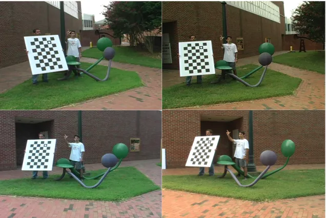
The most common setup for a dynamic scene reconstruction consists of multiple cameras mounted on diﬀerent ﬁxed locations, such as tripods, looking at a common viewing region, as shown in Fig. 1.1. This is because a dynamic scene is theoretically a 4D spatiotemporal continuum, which cannot be captured by a single camera with only 3D sampling ability (2D image frames over time).

Figure 1.1: 1 Multi-camera network setup. Outdoor data capturing with 9 video cam-corders behind the Ackland Museum, UNC-Chapel Hill, 2006/8/24.

(16)

Over the past decades, people have proposed effective ways to recover 3D dynamic shapes in indoor laboratory environment with constant lighting, uniform-colored static background, empty viewing space without any visual occluders, etc. However, one cannot extend such systems directly to an uncontrolled natural environment. A natural scene is far more complicated with environmental variations, including sunlight changes, soft shadows casted by clouds, dark shadows cast by trees or dynamic shapes themselves, visual occluders that are common in outdoor scenes, varying background possibly with fluttering tree leaves or passing-by people at distance, reflections on glassy or metallic surfaces, etc.

This thesis contributes algorithms to address diﬀerent aspects of the uncontrolled 3D dynamic scene modeling. Although diﬃcult, the challenges have to be conquered, as it is believed that in order to realize the previously mentioned real-world applications, the system has to work outside of the laboratory ultimately.

1.2 Thesis Statement

3D dynamic scenes in an uncontrolled natural environment can be robustly and effi-ciently reconstructed with a multi-view sensor network using a probabilistic occupancy model and Bayesian sensor fusion framework, upon which visual occlusion can be ex-plicitly modeled, static occluders can be automatically recovered, individual shapes can be distinctively estimated and tracked, and effective spatiotemporal analysis can be conducted to compute 3D dense motion field and refine the recovered shapes. More-over, heterogeneous sensors can be easily integrated in the mathematical computation framework.

1.3 Contribution

(17)

1. 3D static occluder automatic recovery.

An algorithm is introduced that robustly estimates the shape of static occluders given only silhouette cues of dynamic shapes. The algorithm is built upon the existing probabilistic occupancy volume algorithm for dynamic shape estimation. In addition to the dynamic shape occupancy probability grid, a second probability grid of the static occluders is introduced and is used to explicitly model the visual occlusion event. With dynamic shapes’ arbitrary activity in the scene, the shape of the occluder is automati-cally accumulated over time.

2. Simultaneous multiple shape estimation and tracking.

An algorithm is presented to reconstruct and track multiple dynamic shapes, such as a group of people. An appearance model of each individual shape is automatically learned when it ﬁrst enters the scene. Similar to the static occluder recovery, the inter-occlusion event between the dynamic shapes is explicitly modeled. At every time instant, an object’s location is also tracked and updated.

3. Dense 3D motion ﬁeld recovery.

(18)

4. Heterogeneous sensor network of video camcorders and Time-of-Flight

sensors for dynamic scene reconstruction.

Methods are presented that, as long as the probabilistic sensor model can be deﬁned for shape reconstruction purpose, a sensor fusion framework can seamlessly combine the heterogeneous sensor observations together, which is robust against noise and many challenging scene variations. An example of a network of oﬀ-the-shelf video camcorders and technologically-new-but-highly-potential Time-of-Flight(ToF) sensors are tested as an example of the theory. ToF cameras are a relatively new technology that have become widely available in the last decade. One of their features is the ability to directly acquire 2.5D depth images at video frame rates. An automatic scheme to calibrate the extrinsics of such heterogeneous network is also provided, despite the low imaging resolution drawback of the current ToF sensor technologies to the traditional checkerboard or laser-pointer calibration schemes.

1.4 Overview

The remainder of the dissertation is organized as follows.

Chapter 2 presents the background and fundamental technologies required for multi-view reconstruction and an overmulti-view of the existing and related terminologies. First, camera network calibration is discussed. Second, two types of reconstruction algorithms, the silhouette-based method and the multi-view stereo are described and compared. Finally, the mathematical foundation for the occupancy estimation, the Bayesian sensor fusion model is described in detail.

Chapter 3 describes a novel method for automatic and robust 3D static occluder re-construction with only dynamic shapes moving within the scene over time. Applications include automatic 3D scene discovery and automatic camera-view selection.

(19)

tracking of multiple dynamic shapes. Appearance models for each individual shape is automatically learned when it ﬁrst appears in the scene, and static occluder recovery is also smoothly integrated in the framework.

Chapter 5 presents a new algorithm to compute a dense 3D motion field given the probabilistic occupancy volumes computed at two consecutive time instances. The mo-tion field is computed as a posterior probability maximizamo-tion problem, which is com-patible with the introduced probabilistic sensor fusion framework. The recovered motion field can be used to refine the occupancy estimation and to generalize the underlying skeletal structure of the dynamic shape.

Chapter 6 describes the sensor model of a Time-of-Flight(ToF) camera and how it can be integrated in the Bayesian sensor fusion framework for dynamic scene reconstruc-tion. As a matter of fact, a ToF camera is only one of the many examples of possible vision sensors. Others include infrared cameras, laser scanners, stereo cameras etc. It is in general tempting to exploit diﬀerent types of sensors, especially new technologies, because one sensor could compensate for another’s drawbacks. However, due to the heterogeneity of the sensor output format, the fusion of diﬀerent types of sensor data is not straightforward. This chapter takes ToF sensor as an example to show the proposed mathematical framework is suitable for not only camcorder network but also such het-erogeneous sensor networks. An automatic calibration method is also introduced in this chapter for such heterogeneous sensor network.

(20)

Chapter 2 Background

2.1 Multiple View Calibration

For multi-view 3D dynamic scene reconstruction, the most common set up is to have the cameras looking inward at a common viewing region, where a performance happens. The exact conﬁguration parameters for each camera needs to be known in advance. These parameters include intrinsics, such as focal length and aspect ratio, and extrinsics, such as the camera location and orientation in the world coordinates. This pre-process to the reconstruction is the “camera network geometric calibration”. The calibration requires classical tools and concepts of multi-view geometry, including image formation models, epipolar geometry, and projective transformations. In addition, feature detection and matching, as well as estimation algorithms, are required. For all the datasets acquired in this thesis, I use a planar checkerboard pattern as the calibration target. The board is painted with 6×9 120𝑚𝑚by 120𝑚𝑚alternating black and white squares, as shown in Fig. 2.1.

(21)

Figure 2.1: Camera network calibration session of the SCULPTURE outdoor datasets. This is one pose of the checkerboard calibration target. Four of the eight synchronized camera views are shown.

lenses, shutter speed, aperture, gain, white balanceetc., which are nice features to have when shooting in an outdoor environment. They also have more aﬀordable prices.

Although videos are captured from multiple views, the 3D reconstruction is per-formed with one frame from each view at a time instance, as if one is reconstructing different static objects one at a time. Therefore, the different videos must be synchro-nized so that one is using the correct set of images for a specific “static object”. A clapping of hand before and after the calibration session is used as a visual and acoustic event for synchronization of these camcorders which are set to run at the same frame rate. And then approximately 25 to 30 synchronized frames of different checkerboard poses are taken from all the views. Without confusion, both the cameras taking multiple pictures and the camcorders are called “cameras” in the rest of the thesis.

(22)

and the details are not presented here. For the datasets captured in this thesis, I used Jean-Yves Bouguet’s checkerboard calibration method1 _{based on [Zhang (2007)],}

followed with a bundle adjustment to recover the cameras’ poses in the world coordinate system.

The camera intrinsics (focal length, skew, optical center, radial distortion factors) and the extrinsics (translation and orientation) with respect to the checkerboard pose of the first frame can be recovered. Since this checkerboard pose is the same across the synchronized camera views, it can be treated as the basis of the world coordinate system and the camera network extrinsics in that frame are thus recovered. Since cameras facing opposite to one another would be impossible to see the same checkerboard pose, in practice, three to four cameras with small enough viewing angle difference are calibrated as one group. Multiple calibration groups are carried out to recover the complete camera network, as long as there are overlapping cameras in the groups that can link all groups together. Followed with a final global bundle adjustment of the complete camera network parameters.

A more convenient approach that can calibrate the complete set of cameras all at once is introduced in [Svoboda et al. (2005)], which uses a laser pointer or a diﬀuse light bulb as a calibration target and moves it around the reconstruction space. The method works well with synchronized cameras indoors. However tracking a laser dot or a light bulb in outdoor sunlight is not very robust. In Chapter 6 an extension of this method using a big spherical calibration target is introduced to calibrate heterogeneous network of camcorders and ToF cameras, which has very low image resolution and only respond to light that is emitted from the sensor itself.

Recently, visual content, such as observations of a dynamic subject’s silhouette, have been used to calibrate large-scale camera networks [Sinha et al. (2004)]. This method only requires a dynamic shape, such as a person, moving in the common scene performing

(23)

arbitrary actions. An extension of the method does not require that the cameras are synchronized [Sinha and Pollefeys (2004)]. However, a major constraint for the method is the relatively high quality silhouette segmentation in every view, which is hard to guarantee in natural environment as discussed later on in this chapter.

2.2 Dynamic Scene Reconstruction

Given the calibrated camera network, existing methods use various image cues to deduce and construct geometrical object models. The two main cues used frequently are the silhouettes of the object of interest and color consistency information. The former is used to form a 3D approximation shape of the original object, the visual hull. The latter is used to pinpoint and triangulate a surface coherent with the conjunction of observed colors in images. Additional geometrical constraints such as surface smoothness are often used to help deduce the information or ﬁll in the gaps where image data is inconclusive. All existing methods are generally successful in controlled environments, where the lighting is constrained and the viewing conditions used to obtain images of objects are optimal. They, however, face substantial diﬃculties when brought outdoors or in generally unconstrained environments.

2.2.1 Silhouette-Based Methods

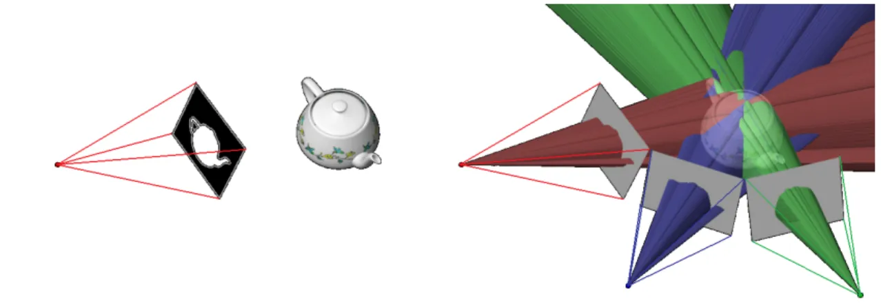
A common approach to multi-view reconstruction uses the silhouettes of objects as sources of shape information. A 2D silhouette is the set of close contours that outline the projection of the object onto the image plane, as well as the regions inside the contours. A common representation is a binary mask image with black being background and white being foreground, as shown on the left of Fig. 2.2.

(24)

Figure 2.2: 1 _{Foreground silhouette and visual hull formation. Left: silhouette of the}

teapot from one view (colored white); Right: back-projection of silhouettes from three views (viewing cones) to intersect the visual hull of the teapot.

shown on the right of Fig. 2.2. The intersection of the viewing cones yields a reasonable approximation of the real object. A “visual hull” is named by [Laurentini (1994)] to describe such intersected volume with inﬁnite number of viewpoints surrounding the actual object.

A visual hull has a few special properties. First of all, it is the maximal object that is consistent with all the silhouettes from the given viewpoints. This property is sometimes called “conservativeness” of the visual hull, because the real shape, which is also consistent with all the silhouettes, is guaranteed to be contained in the visual hull. Secondly, every viewing cone can exclusively eliminate volumes outside of the cone.

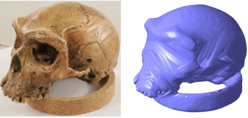
However, no matter how many cameras are used, surface concavities are not re-covered, due to self-occlusion. Notice the diﬀerence between “concavity” and “non-convexity”: a visual hull is able to recover a “saddle region”, which is non-convex, as shown in the teeth dents in Fig. 2.3, while the concave orbital area is never recovered.

One thing to point out is that although the original visual hull concept is based on an inﬁnite number of views, the above properties still hold for the shape recovered from ﬁnite views. In fact, [Baumgart (1974)] originally introduced the visual hull idea with

(25)

Figure 2.3: 1 Left: the same skull model as in Fig. 2.5; Right: its visual hull from 24 images. The non-convex teeth dents are recovered, but not the concavities around the orbital and nasal area.

finite views in his PhD thesis. In the rest of this thesis, we only focus on the visual hull reconstruction algorithms with finite number of views. But they are valid with infinite views in theory.

Shape from silhouettes is a particularly good approach if only an approximate model of the real world is required. The methodology is intuitive and easy to implement. With the advances in computing powers, systems generating real-time 3D digital video for dynamic reconstruction in studio-controlled environment are already on the market, such as [𝑆𝑡𝑎𝑔𝑒𝑇 𝑀 _{(2007), 4}_{𝐷 𝑉 𝑖𝑒𝑤}𝑇 𝑀_{(2008)]. Nevertheless, such systems are restricted}

to a single solid shape within an indoor environment with strictly controlled conditions. All such systems demand on the delicate process of silhouette extraction. If any part of a single silhouette were corrupted, due to the exclusiveness of the viewing cone carving, the corrupted parts would result in incomplete visual hull (which contradicts the visual hull “conservativeness” property) and would never be recovered even if the silhouettes from all other views are correctly computed. Unfortunately, so far, there is no automatic solution that produces silhouettes with the quality as good as manual segmentation. The technical detail about silhouette extraction is introduced later in

(26)

Section 2.3.

2.2.2 Multi-view Stereo

Multi-view stereo algorithms recover 3D surface point locations by triangulating corre-sponding visual features seen from diﬀerent viewing angles, as shown in Fig. 2.4. Once these sparse critical points are recovered, diﬀerent kinds of smoothness constraints can be applied to help recover the whole object surface. A common way to draw the feature correspondences between views is to use the photo-consistency measures [Kutulakos and Seitz (2000)]. Simply put, the resemblance between the pixels/patches in one image to those in the other image is evaluated to see how well the two correlate. A thorough survey is given in [Seitz et al. (2006)].

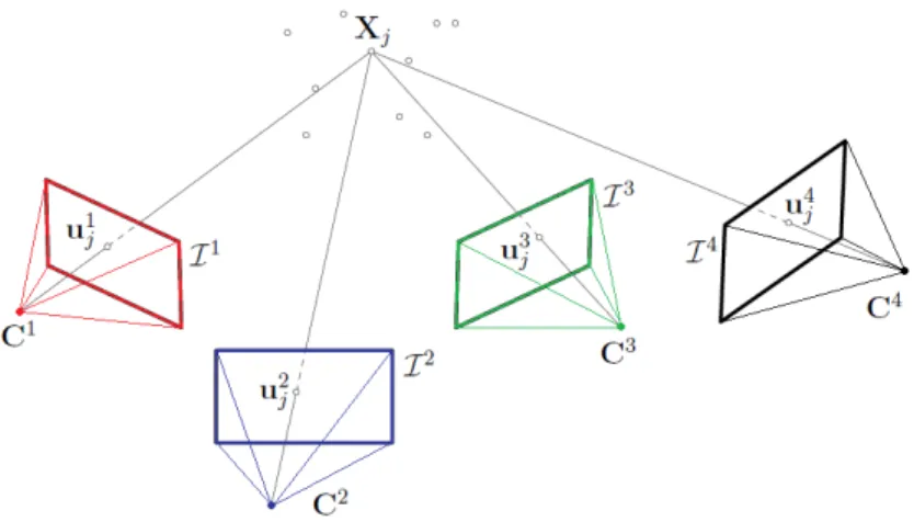
Figure 2.4: 1 Triangulation of 3D point X𝑗 from four camera views. u𝑖𝑗 is the 2D

projection on imageℐ𝑖_{with respect to camera}_C𝑖_{, where the camera index}_𝑖_{∈ {}₁_,₂_,₃_,₄_}_.

Unlike the visual hulls, concave regions can be recovered as long as feature corre-spondences in those regions can be triangulated from diﬀerent camera views, Fig. 2.5 shows a few reconstruction examples. Another major advantage of multi-view stereo is that the recovered surfaces are the exact shapes if triangulation is established for every point on the surface. Therefore, even two views may produce some accurate surface

(27)

fragments, while a two-view visual hull is usually not satisfactory.

However, multi-view stereo algorithms generally only work well on highly textured surfaces, where salient feature points are easy to find. In dynamic scene reconstruction applications, especially human modeling, uniformly colored clothes are very common, thus, it is difficult to find salient features on the person. Fig. 2.6 shows one of the most commonly used scale-invariant features in vision community, the SIFT feature detections [Lowe (2004)], in two sample outdoor frames. Most recovered SIFT features are either on the background structures or at the boundary of the silhouette. The latter unfortunately consists of partial foreground and background pixel information, and thus does not correspond to consistent features from a different view. Therefore, most of the recovered feature points cannot be used to perform 3D triangulation. In situations without many robust features, modern stereo methods, such as [Vogiatzis et al. (2007); Sinha et al. (2007)], have to “reduce” to silhouette constraints with varieties of smoothness regularization.

The second concern is the computation complexity. Unlike the straightforward visual hull algorithms which can reach real-time performance, multi-view stereo algorithms usually involves much slower optimization processes to get the detailed surfaces. From [Middlebury (2009)] dataset evaluation, the fastest GPU accelerated algorithms take tens of seconds to output a ﬁnal shape. It is not generally an issue for static scene modeling, where the reconstruction quality is the main concern. However, for the dynamic scene modeling, these methods are not feasible for real-time applications.

(28)

Figure 2.5: 1 _{The multi-view stereo reconstruction examples.} _Above: _skull

dataset(closed surface); Below: fountain dataset(open surface); Left: one of the original images; Right: recovered surfaces. Notice the bottom row, the shape does not require to be closed when using multi-view stereo.

moved around, but is not practical for dynamic scene modeling where diﬀerent views need to be obtained at the same time. Multiple cameras are thus required to model the latter case.

An additional concern is the color consistency constraint. Besides pixel intensity, pixel color consistency is often used as a multi-view stereo correspondence measure, such as in [Kutulakos and Seitz (2000); Bonet and Viola (1999)]. The multiple color channels contain more information than the pixel intensity and thus produce more ac-curate 3D point correspondence. However, besides many heuristics discussed in [Larsen (2006)], it requires the cameras from all views should be photometrically calibrated. Al-though many advance algorithms have been proposed for camera network photometric

(29)

calibration as in [Kim (2008)], it is in general a tedious manual task [Ilie and Welch (2005)]. The color inconsistency issue has been further investigated in Fig. 4.4 in Chap-ter 4, where one can see how different the views of the same object are in a scene without photometric calibration. Such significant difference normally makes multi-view stereo algorithms fail.

Figure 2.6: The SIFT features extracted for two outdoor frames. Most of the recov-ered salient features are on the silhouette boundary of the foreground shape or in the background.

2.2.3 Comparison and My Choice

(30)

Given the above concerns, the main focus of this thesis is therefore on the challenges of silhouette based methods, especially on how to robustly use silhouette information from multiple views, how to deal with the visual occlusions, how to distinguish multiple dynamic shapes in cluttered environment, and how to eﬀectively make use of temporal consistency given multi-view videos over time.

In the rest of this chapter, I will give an overview of basic automatic silhouette extraction techniques, describing why silhouette extraction is a diﬃcult task in natural scenes. I will also survey silhouette based reconstruction algorithms, including various visual hull representations that researchers have proposed over the years. Among those representations, the probabilistic occupancy grid is the major building block of the algorithms introduced in this thesis.

2.3 Silhouette Extraction

There are mainly two types of algorithms. The ﬁrst uses appearance models such as the active contour shape [Kass et al. (1987)] to compute the silhouette boundary, and track it between frames. These algorithms do not require the cameras be static. But the computation involves energy minimization. Depending on the choice of the appearance measurement and energy design, the tracking result may be slow and may not be the exact desired solution. Overtime, the tracked silhouettes may drift away from the correct shape boundary, especially in some noisy image sequences.

(31)

views. The algorithm itself usually only involves local pixel color examination, which is much easier than active contour energy minimization and involves intensity evaluation of the whole image. The basic background subtraction algorithm [Heikkila and Silven (1999)] as well as the probabilistic modiﬁcation are introduced as follows.

A pixel 𝑝is labeled as the foreground if

ℐ𝑝 − ℬ𝑝 > 𝜏, (2.1)

where 𝜏 is a predeﬁned threshold. Then the binary image is evaluated with a 3×3 kernel to discard small regions.

This simple subtraction inequality only works with an ideal static background. When sensor noise is taken into account, the pixel color observation of the scene is not a constant, but follows a probabilistic sensor model with a certain noise distribution. The most common noise model is an 𝑛-dimensional Gaussian model, where𝑛 is the number of color channels of the pixel readout. Suppose the camera output is an RGB color image, for every pixel, the background color model can be written as

ℬ𝑝 ∼ 𝒩(𝜇𝑅𝐺𝐵,Σ𝑅𝐺𝐵), (2.2)

where 𝜇𝑅𝐺𝐵 and Σ𝑅𝐺𝐵 are respectively the mean vector and covariance matrix of the

RGB channels at𝑝, and𝒩 denotes the normal distribution. ℬ𝑝 explains the probability

of a given pixel color to be background, namely 𝑝(ℐ𝑝∣ℬ𝑝). The probability distribution

can be learned with a few training images in advance. As for the foreground appear-ance modelℱ𝑝 , namely𝑝(ℐ𝑝∣ℱ𝑝), since the dynamic object can take an arbitrary color,

without any prior knowledge, one can assume it to be a uniform distribution. Sup-pose each RGB channel has been discretized to 256 intensity levels, then theoretically

𝑝(ℐ𝑝∣ℱ𝑝) = 1/2563. However, in practice, some colors never show up due to the

(32)

camera. This implies that the colors actually being observed should have greater chance than 1/2563_{. Therefore, usually a constant value} _𝑐 _{larger than 1}_/₂₅₆3 _{is used for the}

uniform distribution. Formally put,

ℱ𝑝 =𝑐 > 1/2563. (2.3)

A pixel 𝑝is labeled as foreground if

𝑝(ℱ𝑝∣ℐ𝑝)> 𝜏. (2.4)

Using Bayes rule, one can easily rewrite the left side of Eq. 2.4 as follows.

𝑝(ℱ𝑝∣ℐ𝑝) =

𝑝(ℐ𝑝∣ℱ𝑝)𝑝(ℱ𝑝)

𝑝(ℐ𝑝)

= 𝑝(ℐ𝑝∣ℱ𝑝)𝑝(ℱ𝑝)

𝑝(ℐ𝑝∣ℬ𝑝)𝑝(ℬ𝑝) +𝑝(ℐ𝑝∣ℱ𝑝)𝑝(ℱ𝑝)

, (2.5)

where𝑝(ℬ𝑝) and𝑝(ℱ𝑝) are the prior probabilities of an image pixel being labeled as the

background and foreground respectively.

Notice the background model described here is a per-pixel model without assuming any spatial consistency between the neighboring pixels. Thus the algorithm is paral-lelizable, and can gain tremendous speedup when ported to a GPU. This is yet another reason to choose the background subtraction algorithm for silhouette extraction. Details about the GPU acceleration are discussed in Chapter 3. Although one could argue for the use of more advanced mathematical tools such as Markov Random Field (MRF) to model the spatial coherences and eliminate a few falsely classiﬁed local pixels, e.g.

[Ahn et al. (2006)], the general per-pixel model described above is the core for most background subtraction algorithms, and is good enough for many applications. The sub-index 𝑝in ℐ𝑝,ℬ𝑝 and ℱ𝑝 are omitted for simplicity afterwards, when not otherwise

speciﬁed.

(33)

often not the case in real environments. With indoor scenes, reflections or soft shadows lead to background changes. Similarly, the static background assumption has difficulties with outdoor scenes, due to wind, clouds, hard shadows, or background motion (motion in the background that is not of the interest, such as tree leaves flickering, people walking at a distance etc.). An example of an outdoor result using Eq. 2.4 is shown in Fig. 2.7, where the shadows and tree leaves are mislabeled as part of the foreground silhouette.

Figure 2.7: The silhouette from background subtraction. Left: an outdoor scene with a person; Middle: the trained mean background; Right: the silhouette(white) by thesh-olding the per-pixel background probability computed from Eq. 2.4. The shadow is labeled as a part of the silhouette.

The background variation problem can be tackled by background updating algo-rithms [Toyama et al. (1999)] and with Gaussian Mixed Models (GMM) instead of the na¨ıve normal distribution [Stauffer and Grimson (1999)]. However, complex background models are computationally more expensive. Additionally, the online update of the back-ground model often gets confused with very slow foreback-ground motion. For example, a seated person would gradually fade into the background, which is not desirable for sil-houette extraction. An alternative is to find robust features. For example, robust color features alleviate the problem of illumination variations, e.g. [Finlayson et al. (1996)], but the trade-off is that a more robust color coordinate often means less discriminative power.

(34)

many scenes. An “occluder” in this thesis context is a potential visual obstacle that, from a certain viewing direction, may be visually occluding the subject to be modeled. For example, the metallic sculpture in Fig. 1.1. Since the sculpture is not movable in this case, the background model trained in advance would have the sculpture as part of the background. Consequently, when a person goes behind the sculpture, the occluded pixels would still take the color of the sculpture, which is consistent with the trained background model. Such phenomenon together with shadows and reﬂections are illustrated in Fig. 2.8. As discussed before, such an incomplete silhouette is disastrous for visual hull construction, because every missing bit in any silhouette view will carve away some part belonging to the real shape.

Figure 2.8: Background subtraction results of incomplete silhouettes outdoors. Left: a person behind the metallic sculpture; Middle: the trained mean background; Right: the foreground silhouette probability without thesholding with black and white denoting 0.0 and 1.0 respectively.

(35)

dilemma: the more cameras used, the better visual hull approximates the real shape, but at the same time, the smaller freedom of motion for the subject. This limits the potential of the multi-view systems in practice. People have come up with algorithms such as camera view selection, which only uses the views that contain the whole subject shape for visual hull construction. But the criterion to determine silhouette completeness is non-trivial. An algorithm that does not require such camera view selection is discussed in Section 2.4.2 and is extended to solve the static occluder problem in Chapter 3.

Second, when the foreground object color happens to be similar to the background color of certain pixels, Eq. 2.4 & 2.5 would classify the pixel as background. In Fig. 2.7, the missing hair at the top of the person is because of this. Given a natural scene, this problem tends to happen only for individual pixels and in individual time instants, but not consistently happen on a speciﬁc foreground region (e.g. the hair) when the subject moves between locations. Therefore, this problem can be largely overcome by consid-ering spatially and temporally neighboring information. It could also be alleviated by a more speciﬁc foreground object appearance model rather than just a uniform fore-ground model as in Eq. 2.3. The ideas mentioned above have been used in algorithms in Chapter 4 and 5.

2.4 Visual Hull Reconstruction

(36)

2.4.1 Deterministic Approaches

Except some hybrid approaches, such as [Boyer and Franco (2003)], most of the de-terministic approaches fall into two categories: (1) surface approaches that focus on a surface representation of the visual hull and (2) volumetric approaches that focus on the volume of the visual hull and usually rely on a discretization of 3D space. A third category exists that computes a view dependent visual hull image from an arbitrary viewpoint [Matusik et al. (2000)]. This method does not require recovery of the explicit 3D models, which although is useful in many applications, is not the major concern of this thesis. All deterministic approaches suﬀer from corrupted silhouette computation.

Surface Representation

The ﬁnal output of this category of algorithms is the visual hull surface, which is cre-ated by analyzing the silhouette boundaries in the images. [Baumgart (1974)] proposed the earliest approach to compute a polyhedral representation of objects from silhou-ette contours, approximated by polygons. A number of approaches assume the local smoothness of the reconstructed surface [Koenderink (1984); Giblin and Weiss (1987); Cipolla and Blake (1992); Vaillant and Faugeras (1992); Boyer and Berger (1997)], and compute the rim points based on a second-order approximation of the surface, from epipolar correspondences.

(37)

to calibration errors or local surface topology near the frontier points have to be dealt with explicitly and carefully.

Volume Representation

A 3D solid volume is the ﬁnal output of this category of algorithms, which is usually in the form of discretized unit cells—the voxels. Unlike surface algorithms, the computation is consistent with the image formation procedure. Every voxel is projected from its 3D location to the silhouette images of every camera view. Only the voxels whose projections fall into the silhouette regions in all camera views are considered visual hull voxels and kept. Others are carved away. After all voxels are evaluated, a discretized visual hull approximation is computed.

Various schemes have been proposed to discretize the 3D space, ranging from the basic ﬁxed grid representations with orthogonal axis-aligned voxels [Martin and Aggar-wal (1983)], to adaptive or hierarchical decompositions of the scene volume [Chien and Aggarwal (1986); Potmesil (1987); Srivastava (1990); Szeliski (1993)]. Some applications have an extra step to extract the object surface from the computed volume, using for example the Marching Cube algorithm [W. Lorensen (1987)].

(38)

2.4.2 Probabilistic Sensor Fusion

Since deterministic visual hull approaches suﬀer from unstable silhouette images, a more robust way of 3D shape estimation is needed for noisy environments such as outdoor scenes. Ideas to compute the visibility probability have been used in shape from photo-consistency and multi-view stereo by [Bonet and Viola (1999); Broadhurst et al. (2001); Yao and Calway (2003)]. A 3D spatial probabilistic occupancy grid concept, borrowed from the robotics community to detect obstacles for robot navigation, is introduced by [Franco and Boyer (2005)] into the shape from silhouette problems. Similar to volume based visual hull approaches, the 3D space is discretized into a regular grid. Instead of a hard decision from binary silhouette images, the algorithm computes the probability of a voxel’s occupancy by fusing the silhouette information from all camera views.

(39)

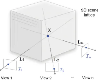
Figure 2.9: Voxel occupancy probability inference overview. Every voxel𝑋 is computed from the observations of all camera views using Bayes’ rule.

Problem Formulation

Consider a single time instant for now. With an orthogonal axis-aligned equal-sized discretization of the 3D space𝒳, for every 3D location𝑋 in𝒳, its probability of being occupied by the dynamic object is computed, given a set of image observationsℐ from𝑛

geometrically calibrated camera views. This occupancy probability is denoted as 𝑝(𝒢𝑋)

with𝒢𝑋 the binary variable at𝑋. The setup is shown in Fig. 2.9, whereL𝑖,𝑖∈ {1, ..., 𝑛},

denotes the 𝑛 viewing lines going through the camera centers and 𝑋.

An intuitive assumption is that diﬀerent views can be independently rendered with-out the knowledge of other views. The background model for one view can be indepen-dently trained.

A second assumption is that the space occupancy variable 𝒢𝑋 ∈ {0,1}depends only

on the information along the optic rays that go through 𝑋, which may include not just the single pixel that the voxel is projected onto, but a 2D neighborhood of pixels around the voxel’s projection.

(40)

Figure 2.10: Occupancy probability inference dependency graph. An arrow points from a source node to a destination node, indicating the destination is caused by or depended on the source node.

is needed. This assumption allows the tractability of the ﬁnal probability computation. This assumption is reasonable also because it has been successful in many deterministic volumetric visual hull algorithms, where every voxel’s status is evaluated individually against its projections onto the image pixels. Results show that the independent com-putation, while not as exhaustive as a global search over all voxel conﬁgurations, still provides very robust and usable shape estimation, at a much lower cost.

The sensor network relationship is modeled as the joint probability 𝑝(𝒢𝑋,ℱ,ℬ,ℐ).

Based on the statistical dependencies expressed in Fig. 2.10, the following decomposition is proposed:

𝑝(𝒢𝑋,ℱ,ℬ,ℐ) =𝑝(ℬ)𝑝(ℱ)𝑝(𝒢𝑋)𝑝(𝒮∣𝒢𝑋)𝑝(ℐ∣ℬ,ℱ,𝒮), (2.6)

where 𝒮 is the binary latent variable introduced to model the silhouette information. Both cases of 𝒮—a pixel being the foreground or background, are considered when computing the ﬁnal occupancy probability, thus maintaining the maximum robustness to silhouette instability.

∙ 𝑝(ℬ),𝑝(ℱ) are the prior probabilities of a pixel to be background and foreground,

which can be approximated statistically by the total background or foreground pixels divided by the number of pixels in the video sequence.

∙ 𝑝(𝒢𝑋) is the prior likelihood for occupancy. Because this occupancy is at the top

(41)

∙ 𝑝(𝒮∣𝒢𝑋) is the silhouette likelihood term. The dependency reﬂects that the voxel

occupancy in the scene explains the object detection in images.

∙ 𝑝(ℐ∣ℬ,ℱ,𝒮) is the image likelihood term. Image colors are conditioned by object

detections in the images, and the knowledge of the pre-learned background and uniformly-distributed foreground color models.

Based on the independence assumptions discussed earlier, Eq. 2.6 can be further decomposed as:

𝑝(𝒢𝑋,ℱ,ℬ,ℐ) = 𝑐

∏

𝑖,𝑝

𝑝(𝒮𝑖,𝑝 ∣ 𝒢𝑋)𝑝(ℐ𝑖,𝑝 ∣ ℱ𝑖,𝑝,ℬ𝑖,𝑝,𝒮𝑖,𝑝), (2.7)

where 𝑐 denotes a constant encoding the uniform prior probabilities discussed before. Once the terms in Eq. 2.7 are explained, the voxel occupancy inference can be carried out following Bayes’ rule as:

𝑝(𝒢𝑋∣ℱ,ℬ,ℐ) =

∑

𝒮𝑝(𝒢𝑋,𝒮,ℱ,ℬ,ℐ)

∑

𝒢𝑋,𝒮𝑝(𝒢𝑋,𝒮,ℱ,ℬ,ℐ)

(2.8)

= ∏

𝑖,𝑝

∑

𝒮𝑖,𝑝𝑝(𝒮𝑖,𝑝 ∣ 𝒢𝑋)𝑝(ℐ𝑖,𝑝 ∣ ℱ𝑖,𝑝,ℬ𝑖,𝑝,𝒮𝑖,𝑝) ∑

𝒢𝑋 ∏

𝑖,𝑝

∑

𝒮𝑖,𝑝𝑝(𝒮𝑖,𝑝 ∣ 𝒢𝑋)𝑝(ℐ𝑖,𝑝 ∣ ℱ𝑖,𝑝,ℬ𝑖,𝑝,𝒮𝑖,𝑝)

.

In Eq. 2.8, 𝑝(ℐ𝑖,𝑝 ∣ ℱ𝑖,𝑝,ℬ𝑖,𝑝,𝒮𝑖,𝑝) is the image formation term. If𝒮𝑖,𝑝 = 1, an object

detection occurred at pixel (𝑖, 𝑝). The pixel color value is explained by the uniform foreground model; if 𝒮𝑖,𝑝 = 0, the pixel color value is explained by the background

model. Both the uniform foreground and Gaussian background models are obtained following Eq. 2.2 & 2.3 respectively.

The only term left in Eq. 2.8 is 𝑝(𝒮𝑖,𝑝 ∣ 𝒢𝑋), the silhouette formation term. It

models the silhouette detection response of a single pixel sensor (𝑖, 𝑝) to the occupancy state of voxel𝒢𝑋. Two local binary hidden variables—sampling variable𝒜and external

(42)

viewing ray of 𝒢𝑋 that may aﬀect the silhouette status. For example, voxel 𝒢𝑋 may

not exactly lie on the viewing line of a pixel, due to potential camera calibration errors, camera mis-synchronization, or simply because a voxel projection is larger than a pixel region. Also, a silhouette may be formed by an object in front of 𝐺𝑋 along the viewing

ray, or sensor noise variations.

When voxel 𝑋 is occupied (𝒢𝑋 = 1), the silhouette detection at pixel (𝑖, 𝑝) is

con-trolled by the sampling variable 𝒜:

𝑝(𝒮∣[𝒢𝑋 = 1]) =𝑝(𝒜= 0) 𝒰(𝒮𝑖,𝑝) (2.9)

+𝑝(𝒜= 1) 𝑃𝑑(𝒮𝑖,𝑝).

By deﬁnition, 𝒜 = 0 if voxel 𝑋 is not on the viewing line of pixel (𝑖, 𝑝). In this case, the knowledge of 𝑋’s occupancy is irrelevant to the sensor detection at (𝑖, 𝑝). Therefore, the uniform distribution 𝒰(𝒮𝑖,𝑝) is used for the silhouette detection in Eq.

2.9. Otherwise, if the voxel is on the viewing line (𝒜 = 1), then the detection at the pixel is ruled by the probability distribution𝑃𝑑(𝒮𝑖,𝑝). In practice, this distribution is set

using a constant 𝑃𝐷 ∈ [0,1], which is a parameter of the system: 𝑃𝑑([𝒮𝑖,𝑝 = 1]) = 𝑃𝐷

is the detection rate of a pixel sensor. 𝑃𝐷 models the silhouette detection rate, as

it happens in practice. The term 𝑝(𝒜) is dependent on 𝑖, 𝑝 and 𝑋. Both uniform sampling and normal based sampling could be used depending on the required accuracy and computation cost.

When voxel 𝑋 is empty (𝐺𝑋 = 0):

𝑝(𝒮∣[𝒢𝑋 = 0]) =𝑝(𝒜= 0) 𝒰(𝒮𝑖,𝑝) (2.10)

+𝑝(𝒜= 1) [ 𝑝(ℰ = 1)𝑃𝑑(𝒮𝑖,𝑝) +𝑝(ℰ = 0)𝑃𝑓(𝒮𝑖,𝑝) ].

(43)

𝑋 is on 𝑝’s viewing line (𝒜 = 1), one needs to also check if there is some other object in front of 𝑋 too. If yes, then pixel (𝑖, 𝑝) is not explained by 𝑋. This is a simple model to explain the visual occlusion relationship along a viewing line. By deﬁnition, ℰ = 1 accounts for the possibility that some other object is on the same viewing line

but in front of 𝑋: in this case, the detection is again ruled by the distribution 𝑃𝑑(𝒮𝑖,𝑝).

However, when no other object obstructs 𝑋 on the viewing line (ℰ = 0), the detection is ruled by the distribution𝑃𝑓(𝒮𝑖,𝑝), which is deﬁned as a constant𝑃𝐹 𝐴 ∈[0,1], another

parameter of the system: 𝑃𝑓([𝒮𝑖,𝑝 = 1]) = 𝑃𝐹 𝐴. It models the false alarm of a pixel

sensor, which occurs when the sensor falsely relates the presence of matter on its viewing line, when in fact there is none. 𝑝(ℰ) is set to be yet another constant. Because there can be detection anywhere along the viewing line of 𝑝, no further assumptions about these causes are made. The constant𝑝(ℰ) means detection is equally likely to be triggered by the voxel occupancy or by the above causes.

Algorithm Experiment and Qualitative Evaluation

In [Franco and Boyer (2005)], an indoor datasetrond of 8 cameras is tested. A person is walking in the scene captured by cameras at diﬀerent image resolutions (640×480 and 780× 580), but at the same frame rate (15 fps). As shown in Fig. 2.11, with

𝑃𝐷 = 0.9, 𝑃𝐹 𝐴 = 0.1, and a uniform sampling 5×5 window for silhouette formation, the

computed occupancy volume itself is a good estimate of the dynamic shape. Although the scene is in a controlled lighting environment, the silhouette segmentations still have artifacts, as shown on the left in Fig. 2.12. But with the introduced probabilistic sensor fusion, most of the system noise does not get much support from another camera at a diﬀerent viewing angle, and therefore is weakened in the ﬁnal result. This phenomenon is the key to the robustness of the algorithm.

The computation in the original paper is approximately 13 sec. per volume on a

(44)

Figure 2.11: 1 _{Color coded 120}3 _{occupancy probability volume of}

rondsequence, with

𝑃𝐷 = 0.9, 𝑃𝐹 𝐴 = 0.1, and a uniform sampling 5×5 window for the silhouette formation.

(45)

2.4 GHz PC. Fortunately, similar to volumetric visual hull algorithms, all voxels in the volume go through exactly the same computation procedure. Therefore, the algorithm is generically parallelizable. A GPU acceleration of this algorithm with the nVidia CUDA𝑇 𝑀 general GPU programming tool is introduced in Chapter 3, which achieves real-time computation with 8 or 9 camera views and a volume size of 1283 _voxels.

Properties of the Probabilistic Sensor Fusion Result

The probabilistic output of the occupancy grid does not strictly follow the “conservative-ness” property of the visual hull [Laurentini (1994)]. In other words, after thresholding the probability volume, the output shape is not guaranteed to contain the entire shape. However, the output can be taken as a robust shape estimate of the original object from multiple camera views.

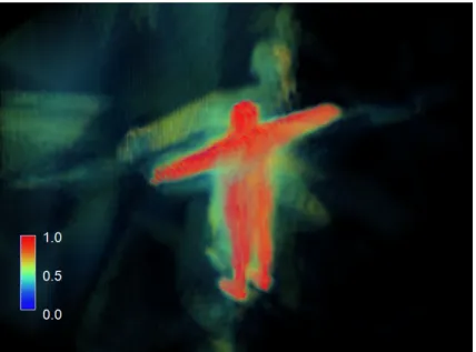
Another property of the occupancy grid is that the recovered shape is not only ro-bust to the sensor noise, but also to the sensor failure or the “out of the ﬁeld of view” scenario. The second row of Fig. 2.12 indeed shows one example, where the person’s arm is out of the camera view. But since most of the cameras see the arm, the ﬁnal 3D shape estimate still have very high occupancy probability at the arm voxels in Fig. 2.11. Therefore, unlike many multi-view systems, such as [Gupta et al. (2007)], this proba-bilistic approach does not require any explicit camera selection when the 3D object is out of view. Moreover, this phenomenon gives some intuition into how to automatically deal with visibility occlusions, as discussed in the following chapters.

(46)

Chapter 3 Static Occluder (Visibility Obstacle)

Inference

In general environments, occlusion is a problem for shape-from-silhouette methods. It can be categorized into (1) static occlusion and (2) dynamic shape inter-occlusion, both of which decrease the reconstruction quality, yet are very common and almost unavoid-able in real sequences. Static occlusion is the main focus of this chapter. Dynamic shape inter-occlusion is discussed in Chapter 4.

3.1 Static Occluder Challenge

(47)

in an incomplete visual hull.

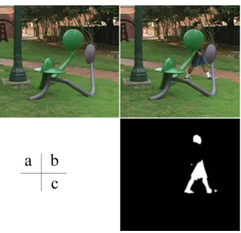
Figure 3.1: Static occlusion problem in silhouette-based reconstruction method. (a) a natural scene with unremovable complicated static occluders; (b) a camera frame during a dynamic scene capturing; (c) manual segmentation of the foreground silhouette.

(48)

of my knowledge, the method introduced in this chapter, based on [Guan et al. (2007)] is the ﬁrst to address the dense recovery of full 3D occluder shapes from multiple image sequences.

Recently, [Keck and Davis (2008)] also proposed to explicitly model static occluders. They use iterative EM framework that at each frame first solves the voxel occupancy which then feeds back into the system by updating the occlusion model. Hard threshold of silhouette information is required during initialization and the occluder information is maintained in a 4D (a 3D space volume per camera view) state space. Also, the usage of iterative refinement makes it only an off-line solution and hard for real-time accelerations. The advantage of [Keck and Davis (2008)], is that it focuses on systems with fewer cameras. Although three to four cameras may still be feasible, [Guan et al. (2007)] use eight or more cameras simply to produce decent shape estimate.

Since publication, the proposed algorithm has been embedded in a dynamic scene reconstruction system which incorporates multiple dynamic shape estimation and track-ing as well as static occluder recovery [Guan et al. (2008b)]. It has been shown that the recovery of occluders does help reﬁne dynamic shapes. More details are discussed in Section 3.4 and Chapter 4.

3.2 Intuition and Solution

(49)

Figure 3.2: Deterministic occlusion reasoning. (a) An occluder-free region 𝒰𝑡 _{can be}

deduced from the incomplete visual hull 𝒱ℋ𝑡 _{at time} _𝑡_{. (b)} _𝒰_{: occluder-free regions}

accumulated over time.

Theoretically, occluder shapes can be accessed with careful reasoning about the visual hull of incomplete silhouettes (Fig. 3.2). Let 𝒮𝑡 _{be the set of incomplete silhouettes}

obtained at time 𝑡, and 𝒱ℋ𝑡 _{the incomplete visual hull obtained using these silhouettes.}

These entities are said to be incomplete because the silhouettes used are potentially corrupted by static occluders that mask the silhouette extraction process. However, the incomplete visual hull is a region that is observed by all cameras as being both occupied by an object and unoccluded from any view. Thus an entire region𝒰𝑡_{of points in space}

can be deduced that are free from any static occluder shape. 𝒰𝑡 _{is the set of points}

𝑋 ∈_ℝ3 _{for which a view} _𝑖 _{exists, such that the viewing line of} _𝑋 _{from view} _𝑖 _{hits the}

incomplete visual hull at a ﬁrst visible point𝐴, and𝑋 ∈𝑂𝐴, with𝑂 the optical center of view 𝑖 (Fig. 3.2 (a)). The latter expresses the condition that 𝑋 appears in front of the visual hull with respect to view𝑖. The region 𝒰𝑡 _{varies with} _𝑡_{, thus assuming static}

occluders and broad coverage of the scene by dynamic object motion, the free space in the scene can be deduced as the region𝒰 =∪𝑇

𝑡=1𝒰𝑡. The shape of occluders, including

concavities if they were covered by object motion, can be recovered as the complement of 𝒰 in the common visibility region of all views (Fig. 3.2 (b)).

(50)

inherent silhouette sensitivity to noise. It also suﬀers from the limitation that only portions of objects that are seen by all views can contribute to occlusion reasoning. In addition, this scheme only accumulates negative information, where occluders are certain not to be. However, positive information is also available to the problem: if one had known or could take a good guess at where the object shape was, discrepancies between the object’s projection and the actual silhouette recorded would tell where an occlusion is happening. Thanks to the sensor fusion occupancy grid introduced in Chapter 2, it can lift these limitations and provide a robust probabilistic solution.

Recall from Section 2.4.2, that the probabilistic occupancy grid has the property that even if a part of the dynamic shape is out of a certain camera’s ﬁeld of view, (e.g. the person’s arm on the bottom row of Fig. 2.12), as long as majority of the cameras see the object, the out-of-view parts still have high occupancy probability, as shown in Fig. 2.11. In fact, one can think of the out-of-view scenario as a special case of static occlusion, that the area outside of a camera ﬁeld of view is equivalent to a big occluder. This robustness is also true for general occlusions. As long as majorities of the camera views can provide correct support, the occupancy grid would have high occupancy probability in the occluded region.

(51)

Given the robust sensor fusion framework for dynamic shape estimation, a second occupancy grid is introduced to model the static occluder probabilistically, in which all negative and positive cues are fused and compete in a complementary way toward occluder shape estimation. Similar to the dynamic shape estimation, this occlusion computation algorithm is also robust to natural scene variations.

3.3 Modeling

Figure 3.3: Occluder inference problem overview. (a) Geometric context of voxel 𝑋. (b) Main statistical variables used to infer the occluder occupancy probability of 𝑋. 𝒢𝑡, ˆ𝒢𝑡

𝑖, ˇ𝒢𝑖𝑡: dynamic object occupancies at relevant voxels at, in front of, behind 𝑋

re-spectively. 𝒪 , ˆ𝒪𝑡

𝑖, ˇ𝒪𝑡𝑖: static occluder occupancies at, in front of, behind 𝑋. ℐ𝑖𝑡, ℬ𝑖:

colors and background color models observed where 𝑋 projects in images.

Consider a scene observed by 𝑛 calibrated cameras. Focus on the case of one scene voxel with 3D position 𝑋 among the possible coordinates in the lattice chosen for scene discretization. The two possible states of occluder occupancy at this voxel are expressed using a binary variable 𝒪. This state is assumed to be ﬁxed over the entire experiment in this setup under the assumption that the occluder is static. Clearly, the regions of importance to infer 𝒪 are the 𝑛 viewing lines L𝑖, 𝑖∈ {1, ..., 𝑛}, as shown in Fig. 3.3(a).

Scene states are observed for a ﬁnite number of time instants𝑡∈ {1, ..., 𝑇}. In particular, dynamic shape occupancies of voxel 𝑋 at time 𝑡 are expressed by a binary statistical variable𝒢𝑡_{, treated as an unobserved variable, which is computed using the formulation}

introduced in Section 2.4.2. Notice that, the subscript𝑋 at 𝒢𝑋𝑡 is omitted from now on

(52)

Observed Variables

The voxel𝑋 projects to𝑛 image pixels𝑥𝑖, 𝑖∈ {1, ..., 𝑛}, whose color observed at time 𝑡

in view 𝑖 is expressed by the variable ℐ𝑡

𝑖 . Assume that static background images were

observed free of dynamic objects, and that the appearance and variability of background colors for pixels𝑥𝑖 was recorded and modeled using a set of parameters ℬ𝑖. Such

obser-vations can be used to infer the probability of dynamic object occupancy in the absence of background occluders. Since the foreground model ℱ still follows the uniform distri-bution, it is omitted for readability. The actual dynamic shape computation is exactly the same as in Section 2.4.2. The problem of recovering occluder occupancy is more complex because it requires modeling interactions between voxels on the same viewing lines. Relevant statistical variables are shown in Fig. 3.3(b).

Viewing Line Modeling

Because of potential mutual occlusions, one must account for other occupancies along the viewing lines of 𝑋 to infer 𝒪. These can be either other static occluder states, or dynamic object occupancies that vary across time. Several such occluders or objects can be present along a viewing line, leading to a number of possible occupancy states for voxels on the viewing line of𝑋. Accounting for the combinatorial number of possibilities for voxel states along𝑋’s viewing line is neither necessary nor meaningful: ﬁrst, because occupancies of neighboring voxels are fundamentally correlated with the presence or absence of a single common object; second, because the main useful information one needs to make occlusion decisions about 𝑋 is whether something is in front of it or behind it, regardless of where the intervening object is along the viewing line.

(53)

of 𝑋with respect to the camera view, if all space from the camera to 𝑋including 𝑋is empty. With this in mind, each viewing line is modeled using three components, the state of 𝑋, the state of occlusion of 𝑋by anything in front and at the back of 𝑋. As mentioned before, neighboring voxels’ states are highly correlated. Namely if a voxel has a high probability of being occupied by a dynamic object, its neighbor is very likely to have a high probability too. Therefore, the front and back components of𝑋are modeled by extracting the two most inﬂuential modes in front and behind of 𝑋, that are given by two voxels ˆ𝑋_𝑖𝑡 and ˇ𝑋_𝑖𝑡 with the highest occupancy probability. We select ˆ𝑋_𝑖𝑡 as the voxel at time 𝑡 that most contributes to the belief that 𝑋 is obstructed by a dynamic object along L𝑖, and ˇ𝑋𝑖𝑡 as the voxel most likely to be occupied by a dynamic object

behind 𝑋 onL𝑖 at time 𝑡.

Viewing Line Unobserved Variables

With this three component modeling, comes a number of related statistical variables illustrated in Fig. 3.3(b). The occupancy of voxels ˆ𝑋𝑡

𝑖 and ˇ𝑋𝑖𝑡 by the visual hull of a

dynamic object at time 𝑡 onL𝑖 is expressed by two binary state variables, respectively

ˆ 𝒢𝑡

𝑖 and ˇ𝒢𝑖𝑡. Two binary state variables ˆ𝒪𝑡𝑖 and ˇ𝒪𝑡𝑖 express the presence or absence of

an occluder at voxels ˆ𝑋𝑡

𝑖 and ˇ𝑋𝑖𝑡 respectively. Note the diﬀerence in semantics between

the two variable groups ˆ𝒢𝑡

𝑖, ˇ𝒢𝑖𝑡 and ˆ𝒪𝑖𝑡, ˇ𝒪𝑡𝑖. The former designates dynamic visual hull

(54)

Figure 3.4: The dependency graph for the static occluder inference at voxel𝑋, assuming the probability for𝑋 to be𝒢 is known. Notice that the background model for each view ℬ𝑖 does not change with time, but just drawn duplicatedly for the clarity of the graph.

3.3.1 Joint Distribution

As a further step toward oﬀering a tractable solution to occlusion occupancy inference, the noisy interactions between the considered variables are described through the decom-position of their joint probability distribution 𝑝(𝒪,𝒢,𝒪ˆ𝑡

𝑖,𝒢ˆ𝑖𝑡,𝒪ˇ𝑖𝑡,𝒢ˇ𝑖𝑡,ℐ,ℬ). According to

the dependency graph shown in Fig. 3.4 the following decomposition of the joint prob-ability is proposed:

𝑝(𝒪,𝒢,𝒪ˆ_𝑖𝑡,𝒢ˆ_𝑖𝑡,𝒪ˇ_𝑖𝑡,𝒢ˇ_𝑖𝑡,ℐ,ℬ) = (3.1)

𝑝(𝒪)

𝑇

∏

𝑡=1

𝑝(𝒢𝑡_∣𝒪₎ 𝑛

∏

𝑖=1

𝑝( ˆ𝒪𝑡

𝑖)𝑝( ˆ𝒢𝑖𝑡∣𝒪ˆ𝑖𝑡)𝑝( ˇ𝒪𝑡𝑖)𝑝( ˇ𝒢𝑖𝑡∣𝒪ˇ𝑖𝑡)𝑝(ℐ𝑖𝑡∣𝒪ˆ𝑖𝑡,𝒢ˆ𝑖𝑡,𝒪,𝒢𝑡,𝒪ˇ𝑡𝑖,𝒢ˇ𝑖𝑡,ℬ𝑖),

where 𝑝(𝒪), 𝑝( ˆ𝒪𝑡

𝑖), 𝑝( ˇ𝒪𝑡𝑖) are priors of occluder occupancy. They are set to a single

constant distribution 𝑃𝑂 which reﬂects the expected ratio between occluder and

Multi-view dynamic scene modeling