Ye_unc_0153D_14302.pdf

DATA-DRIVEN SERVICE OPERATIONS MANAGEMENT

Han Ye

A dissertation submitted to the faculty of the University of North Carolina at

Chapel Hill in partial fulfillment of the requirements for the degree of Doctor of

Philosophy in the Department of Statistics and Operations Research.

Chapel Hill

2014

ABSTRACT

Han Ye: DATA-DRIVEN SERVICE OPERATIONS MANAGEMENT

(Under the direction of Haipeng Shen)

This dissertation concerns data driven service operations management and

in-cludes three projects. An important aim of this work is to integrate the use of

rigorous and robust statistical methods into the development and analysis of service

operations management problems. We develop methods that take into account

de-mand arrival rate uncertainty and workforce operational heterogeneity. We consider

the particular application of call centers, which have become a major

communica-tion channel between modern commerce and its customers. The developed tools and

lessons learned have general appeal to other labor-intensive services such as

health-care.

The first project concerns forecasting and scheduling with a single uncertain

ar-rival customer stream, which can be handled by parametric stochastic programming

models. Theoretical properties of parametric stochastic programming models with

and without recourse actions are proved, that optimal solutions to the relaxed

pro-grams are stable under perturbations of the stochastic model parameters. We prove

that the parametric stochastic programming approach meets the quality of service

constraints and minimizes staffing costs in the long-run.

TABLE OF CONTENTS

LIST OF TABLES

. . . .

vii

LIST OF FIGURES

. . . .

ix

1

Introduction

. . . .

1

2

Stability Analysis on Stochastic Programming Models

. . . .

6

2.1

Background and Motivation . . . .

6

2.2

Model Stability Analysis . . . .

8

2.2.1

Simple Stochastic Program . . . .

9

2.2.2

Later Stage Recourse Program . . . .

13

2.2.3

Two-Stage Recourse Program . . . .

22

2.2.4

A More Generalized Model for the Simple Stochastic Program

27

2.3

Discussion and Future Work . . . .

37

3

Forecasting and Staffing Call Centers with Multiple Arrival Streams

38

3.1

Literature Review . . . .

39

3.2

Statistical Methodology

. . . .

41

3.2.1

Forecasting Model

. . . .

41

3.2.2

Forecasting Error . . . .

44

3.2.3

Forecasting Procedure . . . .

47

3.2.4

Distributional Forecast . . . .

50

3.2.5

Performance Measures . . . .

51

3.3

Staffing Algorithm

. . . .

51

.

.

.

.

.

.

.

. . . . . . . . . . .

.

.

.

.

. .

. .

3.3.1

The Chance Constraint Formulation

. . . .

52

3.3.2

Sampling Process . . . .

55

3.3.3

Performance Measures . . . .

56

3.3.4

Operational Staffing Algorithm Setup . . . .

56

3.4

Simulation Study . . . .

57

3.4.1

Simulation Set-up . . . .

57

3.4.2

Forecasting Comparison . . . .

58

3.4.3

Staffing Comparison . . . .

60

3.5

Real Call Center Data . . . .

66

3.5.1

Background of the Data . . . .

66

3.5.2

Numerical Comparison . . . .

70

3.5.3

Effects of System Designs

. . . .

75

3.5.4

Comparison with Existing Bivariate Forecasting Models . . . .

81

3.6

Discussion . . . .

84

3.6.1

Testing the Staffing Algorithm . . . .

84

3.6.2

Alternative Estimation Method . . . .

85

3.7

Conclusion and Future Work . . . .

87

4

Agent Heterogeneity

. . . .

89

4.1

Heterogeneity in Service Times: Agent Learning Curve Modeling . . .

90

4.1.1

Four Learning-Curve Models . . . .

90

4.1.2

Learning Patterns of Agents . . . .

92

4.1.3

Out-of-sample Prediction of Service Rate . . . .

95

.

.

.

.

.

.

.

.

.

.

.

.

.

.

.

.

.

.

.

.

.

LIST OF TABLES

3.1

Comparison of the staffing performance between MU1 and MU2. . .

63

3.2

Comparison between MU2 and MU1. . . .

66

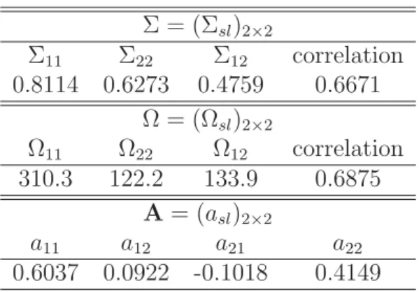
3.3

Some estimates of Model 3.2 on real data.

. . . .

70

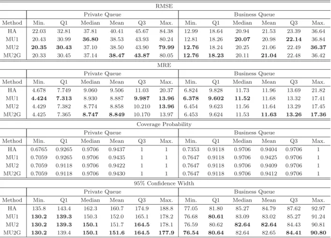
3.4

Comparison of 115 rolling forecasts of RMSE, MRE, Coverage

Prob-ability and Confidence Width.

. . . .

71

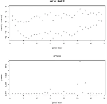
3.5

Paired t-test p-values. . . .

72

3.6

Results of two-sided paired t-test on daily statistics between method

MU2 and MU1. . . .

75

3.7

System parameter settings for the II-design, M-design and X-design.

78

3.8

Staffing comparison in violation probability between MU2 and BME2.

83

3.9

Computation time comparison in seconds. . . .

83

3.10 Violation probability and corresponding p-values for true multi-stream

distribution input and independent single-stream input. . . .

85

3.11 p-values of the paired t-tests. The alternative: additive linear mixed

model is better.

. . . .

87

4.1

Factors considered for the agent-release rate spikes . . . 107

4.2

Significant variables after variable selection. . . 108

.

.

.

.

.

.

. .

.

.

.

.

.

LIST OF FIGURES

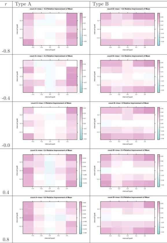
3.1

Simulation comparison on the count RMSE between MU2 and MU1.

Warm color indicates the superior of MU2 in forecasting accuracy of

the counts, and cold color indicates the inferior of MU2 in forecasting

accuracy of the counts. . . .

61

3.2

Simulation comparison on the rate RMSE between MU2 and MU1.

Warm color indicates the superior of MU2 in forecasting accuracy of

the rates, and cold color indicates the inferior of MU2 in forecasting

accuracy of the rates.

. . . .

62

3.3

Staffing performance comparison. Each panel is the scatter plot of

mean interval values between MU1(vertical) and MU2(horizontal).

Each row corresponds to a specific scenario, determined by (r, a

, a

).

Each column corresponds to a performance measure (see column titles). 64

3.4

Staffing performance comparison. Each panel is the scatter plot of

mean interval values between MU1(vertical) and MU2(horizontal).

Each row corresponds to a specific scenario, determined by (r, a12

, a21).

Each column corresponds to a performance measure (see column titles). 65

3.5

Upper: paired t-test C.I. between MU2 and MU1 for each interval.

Lower: paired t-test p-values.

. . . .

67

3.6

Plot for Private customers. Left: arrival volume profiles on

trans-formed scale. Middle: the mean arrival volumes for each day-of-week.

Right: Daily total arrivals on transformed scale.

. . . .

68

3.7

Plot for Business customers. Left: arrival volume profiles on

trans-formed scale. Middle: the mean arrival volumes for each day-of-week.

Right: Daily total arrivals on transformed scale.

. . . .

68

3.8

Dependence between Private and Business customers. Left: scatter

plot for daily totals on the transformed scale with day-of-week

ef-fect removed. Right: scatter plot of interval residual volumes on the

transformed scale with day-of-week and interval effect removed. . . .

69

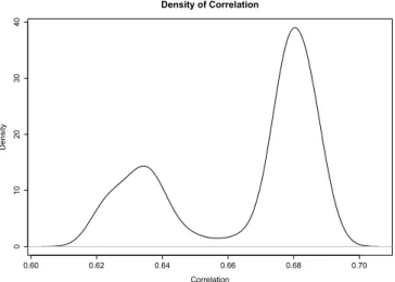
3.9

Density plot of the forecasting count correlation between the two

cus-tomer types.

. . . .

73

.

.

.

.

.

.

3.10 Staffing performance comparison in rolling experiments. Left: Mean

of cost for each time interval. Middle: mean of shortage for each time

interval. Right: violation probability for each tme interval. Horizontal

axis: multiple stream method. Vertical axis: single-stream method. .

75

3.11 Staffing designs. . . .

76

3.12 Real data: daily staffing comparison among the II-design and various

M-designs with different flexible server costs.

. . . .

80

3.13 Real data: daily staffing comparison among the II-design and various

X-designs with different cross service rates.

. . . .

80

3.14 Plot of violation probabilities against correlation for true distributions. 85

4.1

Learning curves for the optimistic case . . . .

93

4.2

Learning curves for the pessimistic case . . . .

94

4.3

Learning curves for the common case . . . .

95

4.4

Prediction errors for Agent 33146 . . . .

97

4.5

Prediction errors for Agent 33147 . . . .

98

4.6

Talk-time distribution. Left: agent-released calls (bimodal pattern is

unusual). Right: customer-released calls (expected pattern). . . 100

4.7

Left: within-day profile of total arrivals. Middle: within-day profile

of agent-released calls. Right: within-day profile of agent-released rate. 100

4.8

Graphic network model for estimating issue resolution rate. . . 102

4.9

Comparison between data-driven and survey-driven estimates. . . 103

4.10 Illustration of our spike detection method. . . 105

.

.

.

.

.

.

.

.

.

.

.

.

1 Introduction

In recent years, call centers have shared a vast industry and are experiencing

dramatic growth. It was estimated in 1999 that the U.S. had 1.55 million call center

agents (Gans et al. (2003)). In 2008, the number of call centers in the U.S. was

estimated to be 47,000 with 2.7 million employees (Aksin et al. (2007)). As a primary

customer-facing communication channel, call centers have become an integral part of

many businesses and are playing an increasingly significant role in bridging service

providers to their customers. It’s estimated that more than 70% of all

customer-business interactions are handled through call centers (Brown et al. (2005)).

The essential challenge for call center managers is to develop efficient staffing and

scheduling strategies to achieve both desired levels of service quality and operating

expenses. The staffing and scheduling process usually begins with forecasting arrival

demand volumes over a planning horizon, which ranges from a day to several weeks.

Call centers also need to evaluate the service quality and efficiency of their agents

during the planning horizon. With the demand forecasts and service evaluation, call

centers then determine the staffing and scheduling plan for short intervals (varying

from 15-min to 1-hour) within the horizon, which minimizes the operational costs

subject to a pre-specified Quality of Service (QoS) level. The final step is rostering

where agents are assigned to the planned schedules.

levels, and further causes the system performance to diverge from operational

tar-get. Recently, people in both statistics and operations management/research have

become aware of the arrival rate uncertainty and have begun to deal with the

prob-lem of the discrepancy between forecasts and realizations. Statistical papers try to

develop more accurate point forecasts and at the same time carefully characterize

the arrival rate forecasting distribution. On the other hand, operations

manage-ment researchers incorporate arrival rate uncertainty into the staffing and scheduling

methodologies. Papers are rare that integrate statistical forecasting process and

op-erational staffing/scheduling process to jointly cope with the arrival rate uncertainty

problem. The first two projects of the thesis aim to bridge the gap between existing

statistical and operational research. The first project concerns call centers with a

single arrival stream while the second one concerns call centers with multiple arrival

streams and investigates the benefits of incorporating inter-stream dependence.

to staff multiple-stream call centers in the short run.

In Chapter 3, we consider both forecasting and staffing together to solve a

com-plete multiple-stream call center staffing problem with uncertain arrival demands.

We evaluate our approach on a real call center data set. We also provide theoretical

assessment and simulation tests of our approach under various scenarios. Our study

demonstrates the importance of incorporating dependence structure among arrival

streams in both forecasting and staffing stages. We also show how the performance

of our multiple-stream approach varies by type and strength of dependence among

the streams. Our efforts naturally extend the work of Gans et al. (2012)., Ibrahim

and L’Ecuyer (2012) and Gurvich et al. (2010).

More specifically, we conduct the following analyses.

•

We develop statistical methods to generate simultaneous distributional

fore-casts of multiple arrival streams. In particular, we decompose within-day

ar-rival volumes of each stream into the product of daily-total rate and within-day

proportion profile. We then apply vector time series models to jointly forecast

multiple-stream daily-total arrival rates. Compared with the linear mixed

ef-fect models in Ibrahim and L’Ecuyer (2012), our method is more attractive in

two ways: it models the inter-stream and within-stream dependence in a more

general form; it’s more practicable and faster in computation.

•

We theoretically evaluate the forecasting benefits of incorporating dependence

among the streams under different type and strength of dependence. In

partic-ular, we derive the forecasting variance reduction of the multiple-stream

fore-casting method over the single-stream forefore-casting method, as a function of

inter-stream and within-stream correlations.

streams, we implement the chance-constraint staffing approach with the sample

based approximation of Gurvich et al. (2010). We demonstrate how the

per-formance of this algorithm varies by the direction and strength of dependence

among the streams.

•

We integrate our forecasting method and the chance-constraint staffing

ap-proach as an entire solution to staffing call centers with multiple uncertain

demand streams. We test our approach on a real call center data set.

Re-sults suggest that the multiple-stream approach provides more accurate

dis-tributional forecasts and the follow-up staffing algorithm is closer to meet the

quality-of-service constraint, compared with the single-stream approach which

ignores the inter-stream dependence. We also test our approach under 125

simulated scenarios of different type and strength of inter-stream dependence.

Our results show that: the stronger the dependence on the other streams’ past

information, the better the forecasting performance of the multiple-stream

ap-proach; for negatively correlated streams, the multiple-stream approach saves

money while at the same time provides the same service quality.

Such assumptions are imposed mainly for mathematical tractability. However they

rarely prevail in practice. The empirical analysis of Brown et al. (2005) reveals that

service-times are log-normally distributed (as opposed to being exponential). We

then perform a detailed analysis of agents’ learning-curves, and show various learning

patterns of agents.

2 Stability Analysis on Stochastic Programming Models

In this chapter we concern forecasting and staffing call centers with a single

un-certain arrival stream, regarding which Gans et al. (2012) developed and tested a

combined forecasting and parametric stochastic programming approach which takes

into account arrival rate uncertainty with inter-day and intra-day dependence. Our

work is an extension of Gans et al. (2012). More specifically, we conduct theoretical

analyses on their parametric stochastic programming models.

2.1

Background and Motivation

In this section, we first briefly review the forecasting and stochastic programming

scheduling approach by Gans et al. (2012) and then highlight our motivation.

particular, the main question of interest is: do their models minimize scheduling cost

and satisfy the QoS constraint in the long-run, theoretically? This big question can

be decomposed into three sub-problems:

•

P1) to show the consistency of the statistical parametric forecasts with or

with-out later stage Bayesian updates.

•

P2) to show the stability of the parametric stochastic programming models in

terms of small perturbations of the model parameters (statistical forecasts).

Since the parametric stochastic programming models are formulated as Integer

Programs (IP), the problem P2) is further decomposed to the following two

problems:

–

P2.1) to show the stability of the model IP’s in terms of relaxation to

Linear Programs (LP).

–

P2.2) to show the stability of the relaxed LP’s in terms of small

perturba-tions of the LP parameters (statistical forecasts).

This chapter provides detailed analyses to address problem P2.2).

In the following is a summary of the three parametric stochastic models proposed

in Gans et al. (2012). Regarding problem P2.2), we consider the LP relaxations to

the following three IP’s.

•

Integer Program (IP) (6) in Gans et al. (2012), that solves to get optimal

sched-ules for the planning horizon given the parametric forecasts for the horizon,

subject to the QoS constraint that expected abandonment rate in the planning

horizon less than a threshold.

updates, subject to the QoS constraint that expected later stage abandonment

rate less than a threshold.

•

IP (12) in Gans et al. (2012), that solves to get optimal schedules for the

planning horizon with recourse given the parametric forecasts for the horizon,

subject to the QoS constraint that expected abandonment rate in the planning

horizon less than a threshold. This model provides optimal schedule before the

planning horizon, consolidating all possible recourse actions for the later stage

before the early stage is observed, compared to (6) and (10) in Gans et al.

(2012).

All the LP relaxations to the above IP’s are driven by the arrival forecasts, in

particular the discretized forecasting distribution. It is non-trivial to substantiate the

existence of optimal solutions to the LP relaxations and that the optimal solutions

are stable with respect to small perturbations of the discretized forecast distribution,

as well as the way it’s discretized. We then address this problem in next section by

providing theoretical stability analysis for the LP relaxations of the above IP’s.

2.2

Model Stability Analysis

Theorem 1 (Robinson (1977), p.440)

The following are equivalent:

(a) The sets

S

and

S

of optimal solutions of (P) and (D) respectively, are

nonempty and bounded. Or equivalently, the conditions R1) and R2) are satisfied:

R1) for every vector

y

= 0,

y

≥

0,

Ay

≤

0 =

⇒

cy <

0, and

R2) for every vector

ρ

= 0,

ρ

≥

0,

ρA

≥

0 =

⇒

ρb >

0.

(b) There exists an

>

0

such that for any

A

,

b

and

c

with

≡

max

{||

A

−

A

||

,

||

b

−

b

||

,

||

c

−

c

||}

<

,

the two dual problems (P

):

max

{

c

x

|

A

x

≤

b

;

x

≥

0

}

and (D

):

min

{

πb

|

πA

≥

c

}

are solvable.

If these conditions are satisfied, then there exist constants

∈

(0,

]

and

γ

such

that for any

A

,

b

and

c

with

<

, any optimal solutions

x

solving

(P

)

and

u

solving

(D

), one has d[(x

, u

), S

×

S

]

≤

γ

.

2.2.1

Simple Stochastic Program

α

’s, that will be useful in our analysis.

min

c

x

subject to

(

a

x

)m

+

b

≤

α

i

∈ I

, k

∈ K

, n

∈ N

i∈I

α

≤

α

k

∈ K

k∈K

p

α

≤

α

¯

λ

x

∈

Z

_j

_{∈ J}

α

≥

0

i

∈ I

, k

∈ K

α

≥

0

k

∈ K

.

(2.1)

Note that, by construction,

m

<

0 and

b

>

0 for all

i,

k, and

n. To avoid

technical distractions, we’ll assume that

c

>

0 for all

j

∈ J

,

λ

>

0 for all

i

∈

I

, k

∈ K

and that

p

>

0 for all

k

∈ K

. That is, the cost of people working on any

schedule is strictly positive, as is the expected number of arrivals under any of the

problem’s scenarios and their probabilities.

We would like to prove the following proposition so that that the objective value

and

α

’s obtained by the optimal solution to the above IP are continuous with respect

to perturbations of the parametric forecasts

p

’s and

λ

’s.

a standard form:

min

c

x

subject to

(

a

x

)m

−

α

≤ −

b

i

∈ I

, k

∈ K

, n

∈ N

i∈I

α

−

α

≤

0

k

∈ K

k∈K

p

α

≤

α

λ

¯

x

≥

0

j

∈ J

α

≥

0

i

∈ I

, k

∈ K

α

≥

0

k

∈ K

.

(2.2)

Here’s the vector-matrix form of the above LP

max

−

cx

+ 0α

_{+ 0α}

subject to

⎡

⎢

⎢

⎢

⎢

⎣

A

A

A

A

A

A

A

A

A

⎤

⎥

⎥

⎥

⎥

⎦

⎡

⎢

⎢

⎢

⎢

⎣

x

α

α

⎤

⎥

⎥

⎥

⎥

⎦

≤

⎡

⎢

⎢

⎢

⎢

⎣

−

b

0

α

¯

λ

⎤

⎥

⎥

⎥

⎥

⎦

x, α

_{, α}

≥

_0.

(2.3)

The decision variables are as follows:

•

x, a

|J |

-vector;

•

α

_{, a}

_{|I| · |K|}

_{-vector of the}

_α

ik

’s; and

•

α

_{, a}

_|K|

_{-vector of the}

_α

k

’s.

The right-hand-side has three parts:

•

α

λ, a scalar

¯

and the constraint matrix is made up of the following submatrices, each with

di-mensions that match the corresponding segments of the right-hand side and decision

variables:

1)

A

, a matrix of 0’s and

m

’s, where each slope

m

<

0;

2)

A12, a matrix of

−

1’s and 0’s;

3)

A13, a matrix of 0’s;

4)

A

, a matrix of 0’s;

5)

A

, a matrix of 1’s and 0’s;

6)

A

=

−

I, the negative of the identity matrix;

7)

A

, a row vector of 0’s;

8)

A

, a row vector of 0’s; and

9)

A

, a row vector of

p

’s.

For condition R1, we let

y

= (x, α

_{, α}

_{) be such that}

_y

_{= 0 and}

_y

_≥

_{0. We note}

that only

α

_{= 0 ensures that the left-hand side of the constraint}

k∈K

p

α

≤

α

λ

¯

is

not positive. In turn, given

α

_{= 0 only}

_α

_{= 0 ensures that the left-hand sides of the}

constraints

α

−

α

≤

0 (for all

k

∈ K

) are not positive. Thus if

y

= 0, there

must be an

x

>

0 so that

−

c

x

<

0. Thus

cy <

0, and

y

satisfies the conditions of

R1.

since there will be an element

m

<

0 of

A

that is multiplied with

ρ

and both

A21

and

A31

have all zeros. In this case, R2 is trivially satisfied. If

ρ

= 0 and

ρ

>

0,

then

ρ

_α

_{λ >}

¯

_{0 implies that (ρ}

_{, ρ}

_{, ρ}

₎₍

₋

_b,

_{0, α}

_λ)

¯

_>

_{0 and again R2 is satisfied. If}

ρ

_{= 0 and}

_ρ

_{= 0, then there must be a}

_ρ

k

>

0, and in this case

(ρ

, ρ

, ρ

)

⎡

⎢

⎢

⎢

⎢

⎣

A

A

A

⎤

⎥

⎥

⎥

⎥

⎦

<

0

since the

kth column of

A

is all 0’s, and the

kth column of

A

has a

−

1’s in the

kth row and 0’s elsewhere. Again, R2 is trivially satisfied in this case.

Thus the LP relaxation (2.2) satisfies R1 and R2 and, and the optimal solutions

are continuous with small but arbitrary perturbations of the LP 2.2.

2

2.2.2

Later Stage Recourse Program

max

−

j∈J

h∈Hj

d

z

subject to

j∈J

h∈Hj

r

m

z

−

α

≤ −

b

−

(

j∈J

a

x

)m

i

∈ I

, k

∈ K

, n

∈ N

i∈Il

α

−

α

≤

0

k

∈ K

k∈K

p

α

≤

α

˜

h∈Hj

z

≤

x

j

∈ J

z

∈

Z

_j

_{∈ J}

_{, h}

_{∈ H}

j

α

≥

0

i

∈ I

, k

∈ K

α

≥

0

k

∈ K

(2.4)

Where ˜

α

=

k∈K

p

i∈Il

(s

·

m

+

b

) is the expected abandonment rate of the

later stage that would have been achieved by the original scheduling policy, and

s

≡

j∈J

a

x

denotes the early stage staffing levels. Without loss of generality, we

assume that

x

>

0 for all

j

∈ J

, otherwise, we could reorganize the schedule set

J

to exclude those

j’s with

x

= 0. Notice that

f

(λ

, μ, θ, n) is non-increasing and

convex in

n

and positive. Then we have

n

·

m

+

b

≤

n

·

m

+

b

,

for all

i

∈ I

, k

∈ K

, n, n

∈ N

.

The LP relaxation of (2.4) is as follows,

max

−

j∈J

h∈Hj

d

z

subject to

j∈J

h∈Hj

r

m

z

−

α

≤ −

b

−

(

j∈J

a

x

)m

i

∈ I

, k

∈ K

, n

∈ N

i∈Il

α

−

α

≤

0

k

∈ K

k∈K

p

k

α

≤

α

˜

h∈Hj

z

≤

x

j

∈ J

z

≥

0

j

∈ J

, h

∈ H

α

≥

0

i

∈ I

, k

∈ K

α

≥

0

k

∈ K

(2.5)

modified LP of (2.5):

max

−

j∈J

h∈Hj

d

z

subject to

j∈J

h∈Hj

r

m

z

−

α

≤ −

b

−

(

j∈J

a

x

)m

i

∈ I

, k

∈ K

, n

∈ N

i∈Il

α

−

α

≤

0

k

∈ K

k∈K

p

k

α

≤

α

h∈Hj

z

≤

x

j

∈ J

z

≥

0

j

∈ J

, h

∈ H

α

≥

0

i

∈ I

, k

∈ K

α

≥

0

k

∈ K

,

(2.6)

and prove the stability of the optimal solution to the LP (2.6). We would like to

make the following proposition:

Proposition 2.2

There exist optimal solutions to the LP (2.6), and the optimal

solutions are stable under small perturbations of the LP (2.6).

Proof

Denote the matrix form of (2.6) by

max

−

dz

subject to

j∈J

|H

|

|I

| × |K

|

|K

|

⎛

⎜

⎜

⎜

⎜

⎜

⎜

⎜

⎜

⎜

⎜

⎜

⎜

⎜

⎜

⎜

⎜

⎜

⎜

⎜

⎜

⎝

⎞

⎟

⎟

⎟

⎟

⎟

⎟

⎟

⎟

⎟

⎟

⎟

⎟

⎟

⎟

⎟

⎟

⎟

⎟

⎟

⎟

⎠

i∈Il

|K

_||N

i

|

(m

r

)

−

I

⊗

1

. ..

−

I

⊗

1

l

|K

_|

_I

K

. . .

I

−

I

1

p

. . .

p

|J |

1

. ..

1

⎡

⎢

⎢

⎢

⎢

⎣

z

α

α

⎤

⎥

⎥

⎥

⎥

⎦

≤

⎡

⎢

⎢

⎢

⎢

⎢

⎢

⎢

⎢

⎢

⎢

⎢

⎢

⎢

⎢

⎢

⎢

⎢

⎢

⎢

⎢

⎣

⎤

⎥

⎥

⎥

⎥

⎥

⎥

⎥

⎥

⎥

⎥

⎥

⎥

⎥

⎥

⎥

⎥

⎥

⎥

⎥

⎥

⎦

g

0

α

x

z

,

α

_,

_α

_≥

₀

(2.7)

Where

d

= (d11, . . . , d1

, . . . , d

),

z

= (z11, . . . , z1

, . . . , z

)

_,

α

_{= (α}

11

, . . . , α

, . . . , α

, . . . , α

)

T

_,

_α

_{= (α}

1

, . . . , α

)

. Further denote the

matrix form as

max

−

dz

subject to

⎡

⎢

⎢

⎢

⎢

⎢

⎢

⎢

⎣

A

A

A

A

A

A

A

A

A

A41

A42

A43

⎤

⎥

⎥

⎥

⎥

⎥

⎥

⎥

⎦

⎡

⎢

⎢

⎢

⎢

⎣

z

α

α

⎤

⎥

⎥

⎥

⎥

⎦

≤

b

z

,

α

_,

_α

_≥

_0.

(2.8)

For condition R1), let

y

=

⎡

⎢

⎢

⎢

⎢

⎣

z

α

α

⎤

⎥

⎥

⎥

⎥

⎦

, and

y

≥

0.

(A

, A

, A

)

y

≤

0

⇒

z

= 0.

(A

, A

, A

)

y

≤

0

⇒

α

= 0,

(A

, A

, A

)

y

≤

0

⇒

α

= 0,

Then

y

= 0 and R1) holds.

For condition R2), the proof is more complex. Firstly LP (2.7) is feasible. In

particular,

z

= 0,

α

=

s

·

m

+b

,

α

=

i∈Il

α

form a feasible solution to (2.7).

Let

z

,

α

, and

α

denote any feasible solutions to (2.7). Let

ρ

= (

ρ

_,

_ρ

_{, ρ}

_,

_ρ

₎

such that

ρ

≥

0,

ρ

= 0 and

ρ

A

≥

0. Notice that

ρ

A

≥

0 is equivalent to the following

three inequalities.

ikn

ρ

m

r

+

ρ

≥

0,

j

∈ J

(2.9)

−

n

ρ

+

ρ

≥

0,

i

∈ I

, k

∈ K

(2.10)

−

ρ

+

p

ρ

≥

0,

k

∈ K

.

(2.11)

To show that R2) holds, we consider four situations:

4)

ρ

_{= 0 and}

_ρ

_{= 0.}

Firstly, by (2.11) we have

ρ

>

0.

Notice in the primal that

x

≥

h

z

, then

ρ

b

=

i

k

n

ρ

−

b

−

(

j

a

x

)m

+

ρ

α

+

j

ρ

x

≥

ρ

−

b

−

(

j

a

x

)m

+

ρ

α

+

j

h

ρ

(2.12)

z

,

where equality holds if and only if

ρ

x

=

ρ

h

z

, j

∈ J

.

In the primal,

j

a

x

+

h

r

z

m

+

b

≤

α

, then

(2.12)

≥

i,k,n

ρ

j,h

r

m

z

−

α

+

ρ

α

+

j,h

ρ

z

,

(2.13)

where equality holds if and only if

ρ

j

a

x

+

j,h

r

z

m

+

b

=

ρ

α

,

i

∈ I

, k

∈ K

, n

∈ N

.

By (2.9), we have

(2.13) =

j,h

z

ρ

+

i,k,n

ρ

m

r

+

ρ

α

−

i,k,n

ρ

α

≥

ρ

α

−

i,k,n

ρ

α

,

(2.14)

where equality holds if and only if

z

ρ

+

i,k,n

ρ

m

r

= 0, j

∈ J

, h

∈

H

.

By the second and third constraints in the primal, we have

(2.14)

≥

ρ

k

p

α

−

i,k,n

ρ

α

≥

ρ

k,i

p

α

−

i,k,n

where equality holds if and only if

α

=

k

p

α

and

i

α

=

α

, k

∈ K

.

By (2.10) and (2.11), we have

(2.15)

≥

0,

where equality holds if and only if

α

ρ

=

α

p

ρ

_{, k}

_{∈ K}

_and

_α

ik

ρ

=

α

n

ρ

, i

∈ I

, k

∈ K

.

Hence,

ρ

b

≥

0 and equality holds if and only if the following equalities hold at

the same time.

ρ

x

=

ρ

h

z

,

j

∈ J

.

(2.16)

ρ

j

a

x

+

j,h

r

z

m

+

b

=

ρ

α

, i

∈ I

, k

∈ K

, n

∈ N

.

(2.17)

z

ρ

+

ikn

ρ

m

r

= 0,

j

∈ J

, h

∈ H

(2.18)

k

p

α

=

α

.

(2.19)

α

=

i

α

,

k

∈ K

.

(2.20)

α

ρ

=

α

n

ρ

,

i

∈ I

, k

∈ K

.

(2.21)

Multiply both sides of (2.19) by

ρ

_{which is positive:}

ρ

α

(2.19)

=

ρ

k

p

α

(2.22)

=

k

ρ

α

(2.20)

=

i,k

ρ

α

(2.21)

=

i,k,n

ρ

α

(2.17)

=

i,k,n

ρ

(

j

a

x

)m

+

b

+

i,k,n

ρ

j,h

r

z

m

(2.18)

=

i,k,n

ρ

(

j

a

x

)m

+

b

−

j,h

z

ρ

(2.16)

=

i,k,n

ρ

(

j

a

x

)m

+

b

−

j

ρ

x

≤

ikn

ρ

(s

m

+

b

)

−

j

ρ

x

≤

ikn

ρ

(s

m

+

b

)

(2.10)

≤

i,k

(s

m

+

b

)ρ

(2)

k

(2.11)

≤

ρ

i,k

(s

m

+

b

)p

.

=

ρ

α

˜

which contradicts the definition of

α

. Hence there must be

ρ

b

>

0.

2

Remark 1

By the proof of Proposition (2.2), we have the following properties for

the LP (2.5) under perturbations of the arrival rate forecasts.

•

For any perturbation of the arrival forecast distribution such that the

p

’s

re-main positive:

R1) holds. Then by Theorem 1 in Williams (1963), the dual is feasible.

Apply-ing Theorem 2 in Williams (1963), there exist optimal solutions to both the

pri-mal and dual. The optipri-mal solution set of the pripri-mal is bounded and the optipri-mal

solution set of the dual is unbounded. In particular, the

ρ

= (

ρ

_,

_ρ

_{, ρ}

_,

_ρ

₎

defined as follows satisfies

ρ

≥

0,

ρ

= 0

,

ρ

A

≥

0

and

ρ

b

= 0:

⎧

⎪

⎪

⎪

⎪

⎪

⎪

⎪

⎪

⎪

⎪

⎪

⎪

⎪

⎪

⎨

⎪

⎪

⎪

⎪

⎪

⎪

⎪

⎪

⎪

⎪

⎪

⎪

⎪

⎪

⎩

ρ

=

⎧

⎪

⎪

⎨

⎪

⎪

⎩

p

n

=

s

,

0

n

=

s

,

i

∈ I

, k

∈ K

,

ρ

=

p

,

k

∈ K

,

ρ

_{= 1,}

ρ

= 0,

j

∈ J

.

2.2.3

Two-Stage Recourse Program

is useful in our analysis.

max

−

j

c

x

−

k

p

j,h

d

z

subject to

(

j

a

x

)m

−

α

≤ −

b

,

i

∈ I

, n

∈ N

(

j

a

x

+

j,h

r

z

)m

−

α

≤ −

b

, i

∈ I

, k

∈ K

, l

∈ L

, n

∈ N

i∈Ie

α

+

i∈Il

l∈Lk

p

α

−

α

≤

0

k

∈ K

k

p

α

≤

α

λ

¯

h

z

−

x

≤

0

j

∈ J

, k

∈ K

x

∈

Z

j

∈ J

z

∈

Z

j

∈ J

, k

∈ K

, h

∈ H

α

≥

0

i

∈ I

, k

∈ K

α

≥

0

i

∈ I

, k

∈ K

, l

∈ L

α

≥

0

k

∈ K

.

Then consider the LP relaxation of (2.23)

max

−

j

c

x

−

k

p

j,h

d

z

subject to

(

j

a

x

)m

−

α

≤ −

b

,

i

∈ I

, n

∈ N

(

j

a

x

+

j,h

r

z

)m

−

α

≤ −

b

, i

∈ I

, k

∈ K

, l

∈ L

, n

∈ N

i∈Ie

α

+

i∈Il

l∈Lk

p

α

−

α

≤

0

k

∈ K

k

p

α

≤

α

λ

¯

h

z

−

x

≤

0

j

∈ J

, k

∈ K

x

≥

0

j

∈ J

z

≥

0

j

∈ J

, k

∈ K

, h

∈ H

α

≥

0

i

∈ I

, k

∈ K

α

≥

0

i

∈ I

, k

∈ K

, l

∈ L

α

≥

0

k

∈ K

.

(2.24)

We would like to make the following proposition for LP (2.24).

Proposition 2.3

The LP relaxation (2.24) is solvable. And the optimal solutions of

the primal and dual are stable under perturbations of this LP.