COMPUTATIONAL APPROACHES TO STUDYING GENE REGULATION USING CHROMATIN ACCESSIBILITY AND GENE EXPRESSION ASSAYS
Bryan C. Quach
A dissertation submitted to the faculty of the University of North Carolina at Chapel Hill in partial fulfillment of the requirements for the degree of Doctor of Philosophy in the Curriculum in Bioinformatics and Computational Biology in the School of Medicine.
Chapel Hill 2017
Approved by:
Terrence Furey
Greg Crawford
Samir Kelada
Karen Mohlke
Praveen Sethupathy
iii ABSTRACT
Bryan C. Quach: Computational approaches to studying gene regulation using chromatin accessibility and gene expression assays
(Under the direction of Terrence Furey)
The completion of the Human Genome Project marked the beginning of a new era in
genomics characterized by significant improvements in high-throughput sequencing technology
and the development of new sequencing-based assays to study a wide array of functional elements
and biological properties at the genome-wide scale. These advancements were accompanied by the
formation of large, multi-institutional consortia that produced publicly available data sets and
functional genomic studies that broadened our understanding of the genome. Previously
uncharacterized genomic regions became recognized as important components of gene regulation,
but the broader knowledgebase of regulatory elements raised new questions to elucidate the
growing complexity of gene regulation models. Additionally, quantitative trait loci (QTL) mapping
approaches began taking advantage of quantitative sequencing data to study the impacts of genetic
variation on molecular phenotypes such as gene expression at the genome-wide level. The
popularity of high-throughput methods for studying gene regulation and transcription lead to a
data deluge that necessitated new statistical methods and bioinformatics solutions for data
management, processing, analysis, visualization, and interpretation. Specialized research areas
emerged to better glean insights from sequencing data leading to new challenges and questions. In
the following chapters, I present a novel machine learning framework for genomic footprinting, a
concept focused on identifying transcription factor (TF) binding sites using chromatin accessibility
iv
binding sites via footprinting. In addition, I investigate characteristics of TF binding sites within
chromatin accessibility data and assess technical factors that influence footprinting to provide an
improved understanding of the strengths and limitations of using these data for TF binding site
prediction. Through a separate study, I investigate the impact of a genotoxic chemical 1,3-butadiene
on chromatin accessibility and gene expression in a population of genetically diverse mice. I
perform expression QTL (eQTL) and chromatin accessibility QTL (cQTL) mapping in these mice and
detect eQTLs and cQTLs in each tissue. In all, the work herein demonstrates multiple computational
approaches to studying various gene regulatory relationships and provides insight on the efficacy of
v
ACKNOWLEDGEMENTS
Firstly, I want to say thank you to my PhD adviser Terry Furey for being a great mentor and
helping shape me as a scientist over the past five years. From troubleshooting broken code and
effectively visualizing results to thinking through the biological interpretation of an analysis, your
wisdom and intuition taught me the necessary skills and mindset to approach the small details of a
problem while also seeing the big picture. I am thankful for the intentionality that you put into
mentoring and teaching students and the sheer number of hours you have endured of me taxing
your brain about research ideas and scientific musings during our meetings.
I also would like to thank my committee members Greg Crawford, Samir Kelada, Karen
Mohlke, Praveen Sethupathy, and Will Valdar for all of your helpful advice and suggestions
throughout various stages of this project. Each of you provided distinct and equally important
perspectives to improve how I framed and approached problems. Additionally, without the help of
members from Greg Crawford and Ivan Rusyn’s labs, none of the 1,3-butadiene project research in
chapter III would have been possible. I want to especially recognize Grace Chappell, Lauren Lewis,
and Alexias Safi. The ATAC-seq and RNA-seq mouse data would not exist without their hard work in
running the mouse experiments and prepping samples.
I also extend my gratitude to the current and former members of the Furey Lab for their
helpful advice and encouragement whenever I hit roadblocks in my research. Special thanks to Karl
Eklund, Jeremy Simon, and Paul Cotney for their work in building the Furey Lab sequencing data
processing pipelines that have proven to be immense time savers. In addition, Greg Keele and Dan
Oreper from the Valdar Lab provided software and expertise that expedited the analysis process for
vi
NIGMS grant T32GM067553, NIEHS grant R01ES023195, and the Lineberger Comprehensive
Cancer Center’s University Cancer Research Fund.
Lastly, thank you to my friends and family near and far for all your love and support
throughout my graduate training. Dad, thanks for always encouraging me in my educational
pursuits and teaching me the life skills that have allowed me to survive under my own roof. Brad
and Jen, thanks for playing host during my visits so that I could experience some of Europe and
recharge my mind without breaking the bank. Matt and Luann, thank you for your love and
encouragement and giving me two awesomely entertaining nephews to wrestle and build Legos
with when I visit. Cherie, I am extremely grateful for your constant support and love. Thanks for
always listening to how my day went and being so attentive. You always brighten my day with your
spontaneous food adventures, and without you, I likely would have spent the last month of
vii
TABLE OF CONTENTS
LIST OF FIGURES . . . viii
LIST OF TABLES . . . xi
LIST OF ABBREVIATIONS . . . xii
I. INTRODUCTION . . . 1
Identifying regulatory elements genome-wide with high-throughput assays . . . 1
Gene expression and chromatin accessibility as quantitative traits . . . 4
The Collaborative Cross as a resource for genetics studies . . .. . .. . .. . .. . .. . .. . .. . . 6
II. DEFCOM: ANALYSIS AND MODELING OF TRANSCRIPTION FACTOR BINDING SITES USING A MOTIF-CENTRIC GENOMIC FOOTPRINTER . . . 9
Introduction . . . 10
Materials and Methods . . . 12
Results . . . 20
Discussion . . . 31
III. CHARACTERIZING MOLECULAR VARIATION IN COLLABORATIVE CROSS MICE AT MULTIPLE LEVELS OF 1,3-BUTADIENE EXPOSURE . . . 66
Introduction . . . 67
Materials and Methods . . . 68
Results . . . 75
Discussion . . . 84
IV. DISCUSSION . . . 147
viii
LIST OF FIGURES
Figure 2.1 Motif logos for NRF1, CHD2, and CEBPB . .. .. .. .. .. . . . .. .. .. .. .. .. .. .. .. .. .. .. . . 34
Figure 2.2 Within and between class variability in DNaseI digestion signal at motif sites . .. .. .. .. .. .. .. .. .. .. .. .. .. .. .. .. .. .. .. .. .. .. .. .. .. .. .. .. .. .. .. .. . . . 35
Figure 2.3 K562 DNaseI signal profiles . .. .. .. .. .. .. .. .. .. .. .. .. .. .. .. .. .. .. .. .. .. .. .. .. . . . 36
Figure 2.4 Coefficients of variation for K562 DNaseI digestion profiles . .. .. .. .. .. .. .. .. .. . . . .37
Figure 2.5 Correlations between aggregate and individual DNaseI digestion profiles . .. .. .. . . 38
Figure 2.6 Pairwise correlation heatmaps for individual DNaseI digestion profiles . . . 39
Figure 2.7 Motif site overlap with ChIP-seq peaks . .. . . 40
Figure 2.8 Overview of the DeFCoM classification framework . .. .. .. .. .. .. .. .. .. .. .. .. .. .. . .42
Figure 2.9 Comparison of DeFCoM model variants . .. .. .. .. .. .. .. .. .. .. .. .. .. .. .. .. .. .. .. . . 43
Figure 2.10 DeFCoM training phase model selection performance . .. .. .. .. .. .. .. .. .. .. .. .. .. . 44
Figure 2.11 Classification performance of DeFCoM-linear vs. DeFCoM-RBF . .. .. .. .. .. .. .. .. .. . 45
Figure 2.12 Comparisons of DeFCoM classification performance with effective and total sequencing depth . .. .. .. .. .. .. .. .. .. .. .. .. .. .. .. .. .. .. .. .. .. .. .. .. .. . 46
Figure 2.13 DeFCoM classification performance on subsampled data . .. .. .. .. .. .. .. .. .. .. .. . . 47
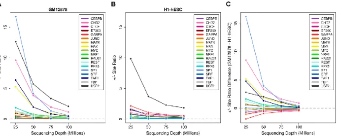
Figure 2.14 Active motif site set size at various sequencing depths . .. .. .. .. .. .. .. .. .. .. .. .. . . 48
Figure 2.15 Active to inactive motif site set size ratio at various sequencing depths . .. .. .. .. .. . 49
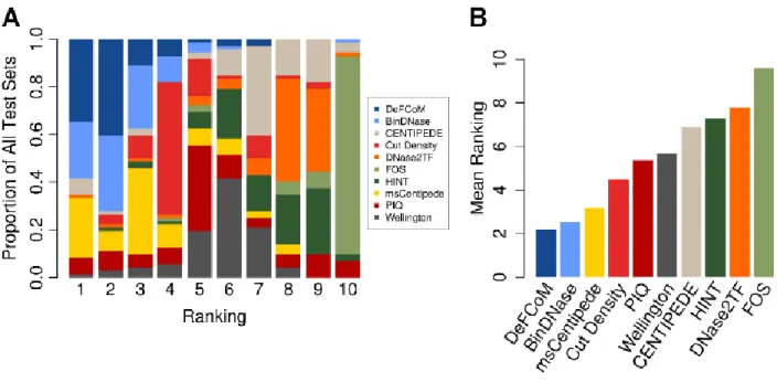
Figure 2.16 Performance ranking of footprinters . .. .. .. .. .. .. .. .. .. .. .. .. . . 50
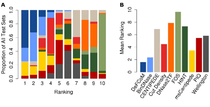
Figure 2.17 Performance ranking of footprinters using cross validation results . .. .. .. .. .. .. .. .51
Figure 2.18 Partial AUC comparison between DeFCoM and Cut Density . .. .. .. .. .. .. .. .. . . 52
Figure 2.19 Performance ranking of footprinters at a 1% FPR cutoff for pAUCs . .. .. .. .. .. .. .. . 53
Figure 2.20 Partial AUC comparison between DeFCoM and BinDNase . .. .. .. .. .. .. .. .. .. .. .. . 54
Figure 2.21 Comparison between using DNase-seq and ATAC-seq with DeFCoM . .. .. .. .. .. .. . 55
ix
Figure 3.2 Multi-tissue gene expression PCA scree plot . .. .. .. .. .. .. .. .. .. .. .. .. .. .. .. .. .. . . 88
Figure 3.3 Multi-tissue gene expression PCA plot colored by tissue type. .. .. .. .. .. .. .. .. .. . . .89
Figure 3.4 Multi-tissue gene expression PCA plot colored by treatment status. .. . . 90
Figure 3.5 Per-tissue gene expression PCA scree plots . .. .. .. .. .. .. .. .. .. .. .. .. . . 91
Figure 3.6 Lung gene expression PCA plot. .. .. .. .. .. .. .. .. .. .. .. .. .. .. .. .. .. .. .. .. .. .. .. . . 92
Figure 3.7 Liver gene expression PCA plot. .. .. .. .. .. .. .. .. .. .. .. .. .. .. .. .. .. .. .. .. .. .. .. . . 93
Figure 3.8 Kidney gene expression PCA plot . .. .. .. .. .. .. .. .. .. .. .. .. .. .. .. .. .. .. .. .. .. .. . . 94
Figure 3.9 Differentially expressed genes by tissue . .. .. .. .. .. .. .. .. .. .. .. .. .. .. .. .. .. .. .. . .95
Figure 3.10 Multi-tissue chromatin accessibility PCA scree plots . .. .. .. .. .. .. .. .. .. .. .. .. .. .. .96
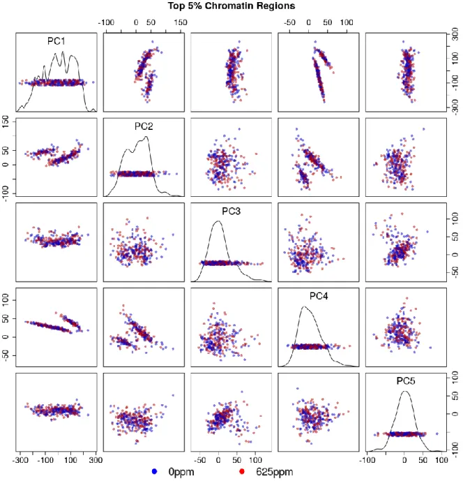
Figure 3.11 Multi-tissue top 5% chromatin windows PCA plot colored by tissue type . .. .. .. .. . 97
Figure 3.12 Multi-tissue top 5% chromatin windows PCA plot colored by treatment status . .. .. .. .. .. .. .. .. .. .. .. .. .. .. .. .. .. .. .. .. .. .. .. .. .. .. .. .. . . 98
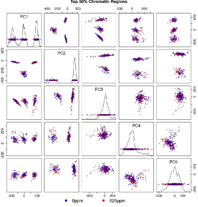
Figure 3.13 Multi-tissue top 50% chromatin windows PCA plot colored by tissue type . .. .. .. .. .. .. .. .. .. .. .. .. .. .. .. .. .. .. .. .. .. .. .. .. .. .. .. .. .. .. .. .. .. .99
Figure 3.14 Multi-tissue top 50% chromatin windows PCA plot colored by treatment status . .. .. .. .. .. .. .. .. .. .. .. .. .. .. .. .. .. .. .. .. .. .. .. .. .. .. .. .. .. . . 100
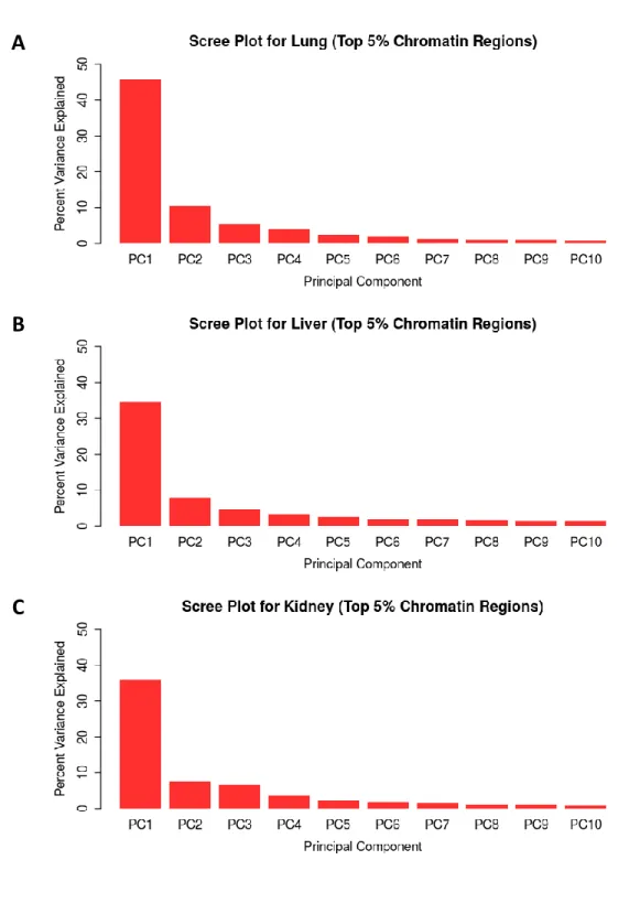
Figure 3.15 Per-tissue top 5% chromatin windows PCA scree plots . .. .. .. .. .. .. .. .. . . 101
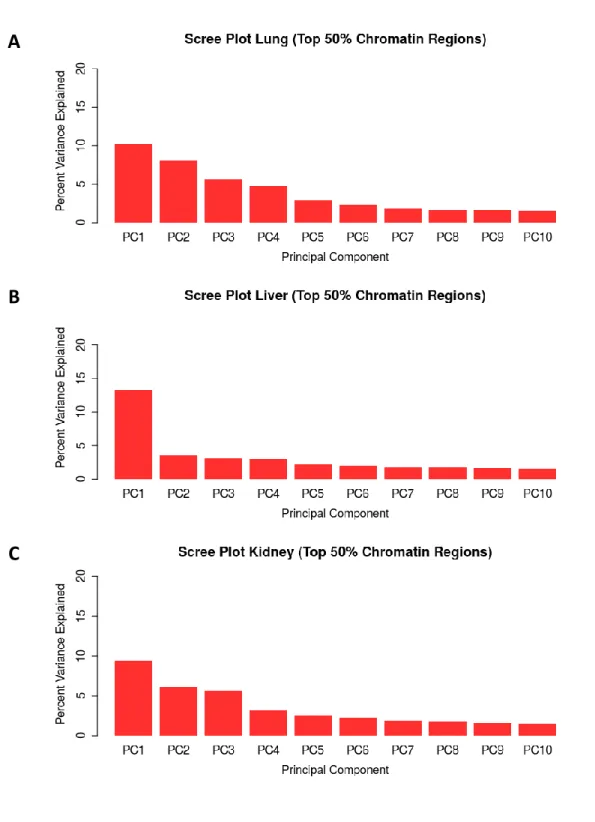
Figure 3.16 Per-tissue top 50% chromatin windows PCA scree plots . .. .. .. .. .. .. .. .. .. . . 102
Figure 3.17 Lung top 5% chromatin windows PCA plot . .. .. .. .. .. .. .. .. .. .. .. .. .. .. .. .. . . . .103
Figure 3.18 Lung top 50% chromatin windows PCA plot . .. .. .. .. .. .. .. .. .. .. .. .. .. .. .. .. . . . 104
Figure 3.19 Liver top 5% chromatin windows PCA plot . .. .. .. .. .. .. .. .. .. .. .. .. .. .. .. .. . . . .105
Figure 3.20 Liver top 50% chromatin windows PCA plot . .. .. .. .. .. .. .. .. .. .. .. .. .. .. .. .. . . 106
Figure 3.21 Kidney top 5% chromatin windows PCA plot . .. .. .. .. .. .. .. .. .. .. .. .. .. .. .. .. . . 107
Figure 3.22 Kidney top 50% chromatin windows PCA plot . .. .. .. .. .. .. .. .. .. .. .. .. .. .. . . 108
Figure 3.23 Distance of eQTL associations . .. .. .. .. .. .. .. .. .. .. .. .. .. .. .. .. .. .. .. .. .. .. .. . . 109
Figure 3.24 Lung control group eQTL map . .. .. .. .. .. .. .. .. .. .. .. .. .. .. .. .. .. .. .. .. .. .. . . . 110
x
Figure 3.26 Kidney control group eQTL map . .. .. .. .. .. .. .. .. .. .. .. .. .. .. .. .. .. .. .. .. .. .. . .112
Figure 3.27 Lung 625 ppm group eQTL map . .. .. .. .. .. .. .. .. .. .. .. .. .. .. .. .. .. .. .. .. .. .. . . 113
Figure 3.28 Liver 625 ppm group eQTL map . .. .. .. .. .. .. .. .. .. .. .. .. .. .. .. .. .. .. .. .. .. .. .. 114
Figure 3.29 Kidney 625 ppm group eQTL map . .. .. .. .. .. .. .. .. .. .. .. .. .. .. .. .. .. .. .. .. .. .. 115
Figure 3.30 Lung 1500 ppm group eQTL map . .. .. .. .. .. .. .. .. .. .. .. .. .. .. .. .. .. .. .. .. .. .. . 116
Figure 3.31 Liver 1500 ppm group eQTL map . .. .. .. .. .. .. .. .. .. .. .. .. .. .. .. .. .. .. .. .. .. .. . 117
Figure 3.32 Kidney 1500 ppm group eQTL map . .. .. .. .. .. .. .. .. .. .. .. .. .. .. .. .. .. .. .. .. .. .118
Figure 3.33 Total fraction of overlapping eQTLs . .. .. .. .. .. .. .. .. .. .. .. .. .. .. .. .. .. .. .. .. . . .119
Figure 3.34 Fraction of overlapping local and distal eQTLs across tissues. .. .. .. .. .. .. .. .. .. . .120
Figure 3.35 Fraction of overlapping local and distal eQTLs across treatment groups . .. .. .. . . . 121
Figure 3.36 Distance of cQTL associations . .. .. .. .. .. .. .. .. .. .. .. .. .. .. .. .. .. .. .. .. .. .. .. .. 122
Figure 3.37 Lung control group cQTL map . .. .. .. .. .. .. .. .. .. .. .. .. .. .. .. .. .. .. .. .. .. .. .. .. 123
Figure 3.38 Liver control group cQTL map . .. .. .. .. .. .. .. .. .. .. .. .. .. .. .. .. .. .. .. .. .. .. .. .. 124
Figure 3.39 Kidney control group cQTL map . .. .. .. .. .. .. .. .. .. .. .. .. .. .. .. .. .. .. .. .. .. .. .. 125
Figure 3.40 Lung 625 ppm group cQTL map . .. .. .. .. .. .. .. .. .. .. .. .. .. .. .. .. .. .. .. .. .. .. .. 126
Figure 3.41 Kidney 625 ppm group cQTL map . .. .. .. .. .. .. .. .. .. .. .. .. .. .. .. .. .. .. .. .. .. .. 127
Figure 3.42 Total fraction of overlapping cQTLs . .. .. .. .. .. .. .. .. .. .. .. .. .. .. .. .. .. .. .. .. .. .128
Figure 3.43 Fraction of overlapping local and distal cQTLs across tissues . .. .. .. .. .. .. .. .. .. . 129
Figure 3.44 Fraction of overlapping local and distal cQTLs across treatment groups . .. .. .. .. . 130
Figure 3.45 Lung control group hotspot haplotype dosages . .. .. .. .. .. .. .. .. .. .. .. .. .. .. .. . . 131
Figure 3.46 Lung 625 ppm group hotspot haplotype dosages. .. .. .. .. .. .. .. .. .. .. .. .. .. .. .. . 132
Figure 3.47 Genome-wide 625 ppm lung and kidney cQTL frequencies . .. .. .. .. .. .. .. .. .. .. . 133
Figure 3.48 Lung chr8 hotspot haplotype dosages . .. .. .. .. .. .. .. .. .. .. .. .. .. .. .. .. .. .. .. .. . 134
xi
LIST OF TABLES
Table 2.1 Summary of footprinters . . . 56
Table 2.2 ENCODE DNase-seq data files . . . 57
Table 2.3 ENCODE ChIP-seq data files . . . 58
Table 2.4 Active and inactive motif site set sizes . . . 63
Table 2.5 Classification performance for DeFCoM training phase variants . . . 64
Table 2.6 DNase-seq signal quality and sequencing depth statistics . . . 65
Table 3.1 Inventory of CC mouse samples . . . 136
Table 3.2 eQTL mapping results overview . . . 145
xii
LIST OF ABBREVIATIONS
ATAC-seq: assay for transposase-accessible chromatin
AUC: area under the curve
BD: 1,3-butadiene
bp: base pair
CC: Collaborative Cross
cDNA: complementary DNA
ChIP-seq: chromatin immunoprecipitation and sequencing
cQTL: chromatin accessibility quantitative trait locus
DeFCoM: Detecting Footprints Containing Motifs
DNA: deoxyribonucleic acid
DNase-seq: DNaseI sequencing
dsQTLs: DNaseI sensitivity quantitative trait locus
ENCODE: Encyclopedia of DNA Elements
eQTL: expression quantitative trait locus
FPR: false positive rate
FRiP: fraction of reads in peaks
GEO: gene expression omnibus
GTEx: Genotype-Tissue Expression
GWA: genome-wide association
HMM: hidden Markov model
LCL: lymphoblastoid cell line
LD: linkage disequilibrium
xiii pAUC: partial area under the curve
PC: principal component
PCA: principal component analysis
ppm: particles per million
PWM: position weight matrix
QTL: quantitative trait locus
RBF: radial basis function
RNA: ribonucleic acid
SNP: single nucleotide polymorphism
SVM: support vector machine
TAMU: Texas A&M University
TF: transcription factor
TFBS: transcription factor binding site
TPM: transcripts per million
UCSC: University of California at Santa Cruz
1 CHAPTER I Introduction
The importance of gene regulation in cell development and biological homeostasis of living
organisms has been well recognized [1–4]. Through the Human Genome Project [5], technological innovations and a broader understanding of genome organization and composition paved way for
large-scale efforts in the genomics community to better understand functional genomic elements and
the role of non-coding DNA in transcriptional regulation [6,7]. Although these efforts improved
understanding of gene regulatory components such as promoters, enhancers, silencers, chromatin
structure, and transcription factors, they also increased awareness of the complexity of regulatory
dynamics and the interactions between the various components. Furthermore, follow-up studies to
quantitative trait loci (QTL) mapping and genome-wide association (GWA) studies that detect
trait-associated genetic variation contributed another layer of regulatory complexity by characterizing
relationships between genetic variation and regulatory changes as intermediate mechanistic links
between DNA sequence and phenotype [4,8]. The increasing availability of information, resources,
methodologies, and technologies for studying gene regulation highlighted a growing opportunity and
significance in further identifying regulatory elements and studying their roles in condition-specific
contexts.
IDENTIFYING REGULATORY ELEMENTS GENOME-WIDE WITH HIGH-THROUGHPUT ASSAYS Since the advent of Sanger sequencing, DNA sequencing technology continued to improve,
and the introduction of massively parallel “next-generation” sequencing approaches revolutionized
2
more cost-effective alternatives to microarrays to assay biological properties such as transcription,
nucleosome occupancy, chromatin interactions, transcription factor (TF) binding, and histone
modifications genome-wide [9]. Although multiple different next-generation sequencing platforms
exist, they share some commonalities in their approach. Each technology first requires the
preparation of a sequence library through the ligation of oligonucleotide adapters to the ends of the
DNA fragments to be sequenced. The fragments are then amplified and undergo a platform-specific
sequencing reaction that allows the classification of each nucleotide. The ability for these reactions
to occur simultaneously leads to the high-throughput that makes them massively parallel. The
nucleotide readouts, referred to as reads, generate large quantities of data that then require the
application of bioinformatics approaches for downstream processing, analysis, and interpretation.
These next-generation sequencing platforms remain widely used, however newer sequencing
platforms are being developed such as nanopore sequencing that rely on different sequencing
chemistry and do not require fragment amplification [10].
From a simplified perspective, sequencing platforms all share the goal of accurately
classifying the nucleotide sequence of the given fragments. The major distinctions in the
sequencing-based methods for assaying different biological properties occur in isolating the
relevant DNA or RNA. For example, Chromatin Immunoprecipitation Sequencing (ChIP-seq) aims to
detect genomic locations of TF occupancy or histone modifications. To do this, binding proteins and
genomic DNA are cross-linked, then the DNA is fragmented. Immunoprecipitation with a
protein-specific antibody retrieves the protein-bound sequences that are then sequenced. Enrichment of
reads mapping to a particular genomic location indicates TF occupancy (or histone modification)
[11]. In DNaseI sequencing (DNase-seq), chromatin accessibility is assayed using the exonuclease
DNaseI. Exposing genomic DNA to DNaseI results in the enzyme preferentially cutting DNA in more
accessible, nucleosome-depleted regions. Following DNaseI digestion, size selected DNA fragments
3
chromatin regions [12]. In both ChIP-seq and DNase-seq, the biomolecule initially being isolated is
DNA. With RNA sequencing (RNA-seq), RNA transcripts are initially isolated as opposed to DNA. For
compatibility with sequencing platforms, these transcripts are typically converted to cDNA before
sequencing, although some direct RNA sequencing approaches exist [13]. The reads from RNA-seq
are mapped to their originating genes and can be analyzed to deduce estimates of RNA abundance.
With the three aforementioned methods, the diversity of biological properties related to
gene regulation that can now be studied genome-wide created new opportunities for
understanding their interactivity. ChIP-seq, DNase-seq, and RNA-seq among other methods were
utilized by the Encyclopedia Of DNA Elements (ENCODE) project which sought to characterize all of
the functional elements in the human genome [7] and in later stages also included the mouse
genome [14]. In a 2012 report, the ENCODE project had produced 1,640 data sets in 147 different
human cell types [15], and a 2014 mouse ENCODE publication comparing the mouse and human
functional elements reported over 1,000 data sets in 123 mouse cell types and primary tissues [14].
Analyses by the ENCODE consortium found that 80.4% of the human genome is covered by at least
one functional element. Of this fraction, RNA-associated elements and histone modifications
comprised a large majority, and 15.2% of the coverage was attributed to DNaseI hypersensitive
sites [15]. In comparisons with mouse functional elements, chromatin state landscapes and TF
networks were found to be relatively stable between human and mouse [14]. Additionally, gene
expression profiles were shown to be more consistent within tissue than within species [16]. To
build upon the work by the ENCODE project, the more recent Roadmap Epigenomics Project
constructed a collection of epigenomic profiles for 127 human tissues and cell types from adult and
embryonic samples [17]. Analyses of these data showed associations between proximal and distal
regulatory regions, histone marks, DNA methylation, chromatin accessibility, spatial organization,
and gene expression that play important roles in cell type identity, development, and disease [17].
4
large-scale projects contributed new insights into the organization and regulation of human and
mouse genes and the genome and continues to serve as an expansive public resource for biomedical
research.
GENE EXPRESSION AND CHROMATIN ACCESSIBILITY AS QUANTITATIVE TRAITS A fundamental challenge in genetics research is to understand genetic variation and its
relationship to phenotypic variability. Efforts such as the International HapMap and 1000 Genomes
Project extensively characterized common genetic variation across diverse human populations
[18,19], and GWA studies have leveraged advancements in genotyping technology to link genetic
variants to human traits and diseases. Although informative in many regards, these studies do not
resolve the underlying biological mechanisms of discovered genotype-phenotype associations. For
functional follow-up, data produced by the ENCODE and Roadmap Epigenomics consortia have
served as valuable resources to refine lists of candidate GWAS variants and identify putative roles
of non-coding variants [20], but these data still do not directly assess the impact of inter-individual
variation on gene regulation and cellular behavior that results in the observed phenotypes.
A related but distinct approach from GWAS is expression QTL (eQTL) mapping. In eQTL
mapping, gene expression levels are treated as quantitative traits and tested for associations with
genetic variants. The first reported eQTL study analyzed over 1,500 genes and 3,312 genetic
markers between two strains of Saccharomyces cerevisiae [21]. Since then, eQTL mapping has been
performed in various contexts using model organisms and humans [22–24]. With RNA-seq (or gene
expression microarrays) and current genotyping approaches, these analyses can include tens of
thousands of genes, each regarded as an independent quantitative molecular phenotype. The
Genotype-Tissue Expression (GTEx) Project pilot analysis demonstrated the utility of eQTL
analyses by performing eQTL mapping in 9 human tissues and identifying eQTLs shared and unique
5
polymorphisms (SNPs) showing whole-blood specific eQTL enrichment for autoimmune-related
GWAS variants [24]. This showed that by directly modeling the relationship between genetic
variation and gene expression, eQTL mapping serves as a powerful tool to gain more insight into
gene regulatory changes that can then be used to elucidate other genotype-phenotype links.
As a complementary approach to eQTL mapping, the genetic underpinnings of chromatin
variation have been studied using sequencing-based assays. Kasowski et al. observed variation
between lymphoblastoid cell lines (LCLs) from 19 individuals for histone modifications H3K27ac,
H3K4me1, H3K4me3, H3K36me3, and H3K27me3. Work by McVicker et al. further assessed the
genetic relationship to histone modifications by identifying SNPs significantly associated with
variation of histone mark signals in LCLs derived from 10 unrelated individuals [25]. Similarly,
Degner et al., used DNase-seq to measure chromatin accessibility in 70 LCLs and detected 8,902
chromatin regions where chromatin accessibility was significantly associated with genotype, which
they referred to as DNaseI sensitivity QTLs (dsQTLs). The dsQTLs discovered were found to be
pre-dominantly local with enrichments for predicted TF binding sites. Sixteen percent of dsQTLs were
also classified as eQTLs, and 55% of identified eQTLs were also dsQTLs. More recently, another
genome-wide chromatin accessibility assay was developed called Assay for Transposase-Accessible
Chromatin Using Sequencing (ATAC-seq) which relies on the Tn5 “tagmentation” process to
fragment DNA at accessible chromatin regions and append adapters for sequencing [26]. Using
ATAC-seq and genotype data from 24 European individuals, Kumasaka et al. reported 2,707
chromatin accessibility QTLs (cQTLs) which were also enriched for eQTLs and dsQTLs [27]. These
QTL analyses using histone marks and chromatin accessibility data as quantitative traits
demonstrate how chromatin assays can contribute to discovering associations between genotype
and gene regulation that can ultimately inform physiologic or disease phenotype-genotype
6
THE COLLABORATIVE CROSS AS A RESOURCE FOR GENETICS STUDIES
In human genetics and genomics studies, certain constraints limit the possible experimental
designs that can be practically realized. As a proxy, various species such as Danio rerio (zebrafish),
Drosophila melanogaster (fruit fly), and mus musculus (mouse) have been studied as model
organisms to infer aspects of human biology [28–30]. In a 2002 review, Threadgrill et al. outlined
propositions made by the Complex Trait Consortium to develop a mouse genetics resource for
effective study of complex traits using QTL approaches [31]. The design and implementation of
creating this resource became known as the Collaborative Cross (CC) [32]. The CC involved an
international, multi-institutional effort to create a multiparent panel of recombinant inbred mouse
strains derived from five classical inbred strains (A/J, C57BL/6J, 129S1/SvImJ, NOD/ShiLtJ, and
NZO/HlLtJ) and three wild-derived strains (CAST/EiJ, PWK/PhJ, and WSB/EiJ) denoted as
“founders”. Because CC strains are inbred, they provide an advantage over human studies in that
each strain can produce genetically identical individuals. This reduces the genotyping burden and
allows for more sophisticated experimental designs to study multiple variables within the same
population.
As described in [32], creating a CC strain requires a funnel breeding scheme that begins
with the mating of the 8 founder strains in pairs. Two pairs from the resulting generation are then
mated, and this process continues for subsequent generations until a final inbred CC strain is
produced. By permuting the pairs in the initial generations, a large number of strains can be
constructed. In an evaluation of the genome architecture of 350 CC strains, similar founder
haplotype representation was observed when averaged across the CC lines, but deviations from
expected frequencies were noted when focusing on specific genomic regions. Unlike many classical
inbred strains, the CC population did not exhibit high levels of long-range linkage disequilibrium
7
[33]. As a proof-of-concept, Aylor et al. performed eQTL mapping using 156 incipient inbred CC
lines (pre-CC) and detected 7,235 liver eQTLs at less than 1 megabase (Mb) resolution. A QTL study
by Kelada et al. used 131 pre-CC lines to identify genetic associations with blood cell volume, white
blood cell count, percentage of neutrophils, and monocyte number [34]. More recently, 45 CC
strains were used to identify liver eQTLs and QTLs associated with treatment response to the drug
tolvaptan. The study showed strain-specific variability in liver toxicity phenotypes and found
several candidate susceptibility genes for tolvaptan drug-induced liver injury [35]. Each of these
studies demonstrates the feasibility and power of the CC as a resource for QTL mapping and
interrogating genetic factors in disease and complex traits.
The significant advancements in systems genetics and functional genomics have made the
intricacies of gene regulation more apparent, fostering new hypotheses for how the contributing
components interact [3,36,37]. The development of sequencing-based assays such as those used by
ENCODE and the Roadmap Epigenomics Project made new types of analyses possible, but in doing
so exposed new questions and challenges to address. Among these challenges is the development of
bioinformatics approaches and statistical methods to manage, process, analyze, and interpret the
vast quantities of biological data being generated. For instance, the development of DNase-seq and
ATAC-seq for detecting accessible chromatin also led to observations that these methods could
probe TF binding locations through an approach called footprinting [26,38], but the strengths and
weaknesses of footprinting have not been well characterized. As previously mentioned, the utility of
the Collaborative Cross for QTL mapping has been demonstrated, but the advantages of the CC can
be further demonstrated by experimental designs and analyses that interrogate both chromatin
accessibility and gene expression under varying environmental conditions.
In chapter II, I introduce a novel method for TF binding site prediction, Detecting Footprints
Containing Motifs (DeFCoM), that integrates DNase-seq or ATAC-seq data with ChIP-seq data and
8
DeFCoM to existing approaches and show that it outperforms other methods. I also evaluate
current assumptions about chromatin accessibility signal characteristics at TF binding sites and
assess the impact of technical factors on footprinting. In chapter III, I present an unpublished
analysis that compares lung, liver, and kidney gene expression and chromatin accessibility for a
control group of CC mice and mice exposed to the chemical 1,3-butadiene. I also characterize eQTLs
and cQTLs in the three tissues to provide a basis for further studies investigating genetic
associations with gene expression and chromatin accessibility in the CC population. In chapter IV, I
discuss how my findings in Chapter II contribute to evaluating footprinting and integrating it into
gene regulation studies, and I conclude the chapter discussing the significance of how my findings
in analyzing CC mice contribute to interrogating environmental exposure and gene regulation in
9 CHAPTER II
DeFCoM: analysis and modeling of transcription factor binding sites using a motif-centric genomic footprinter1
OVERVIEW
Identifying the locations of transcription factor binding sites is critical for understanding
how gene transcription is regulated across different cell types and conditions. Chromatin
accessibility experiments such as DNaseI sequencing (DNase-seq) and Assay for Transposase
Accessible Chromatin sequencing (ATAC-seq) produce genome-wide data that include distinct
“footprint” patterns at binding sites. Nearly all existing computational methods to detect footprints from these data assume that footprint signals are highly homogeneous across footprint sites.
Additionally, a comprehensive and systematic comparison of footprinting methods for specifically
identifying which motif sites for a specific factor are bound has not been performed.
Using DNase-seq data from the ENCODE project, I show that a large degree of previously
uncharacterized site-to-site variability exists in footprint signal across motif sites for a
transcription factor. To model this heterogeneity in the data, I introduce a novel, supervised
learning footprinter called DeFCoM (Detecting Footprints Containing Motifs). I compare DeFCoM to
nine existing methods using evaluation sets from four human cell-lines and eighteen transcription
factors and show that DeFCoM outperforms current methods in determining bound and unbound
10
motif sites. I also analyze the impact of several biological and technical factors on the quality of
footprint predictions to highlight important considerations when conducting footprint analyses and
assessing the performance of footprint prediction methods. Lastly, I show that DeFCoM can detect
footprints using ATAC-seq data with similar accuracy as when using DNase-seq data.
INTRODUCTION
Chromatin dynamics vary based on developmental stage [40], cell type [41], and
environmental stress [42]. Transcription factors (TFs) bind DNA in regions of accessible chromatin
and play a central role in pre-transcriptional gene regulation. Understanding these interactions is
critical in deciphering transcriptional regulation that defines cell identity in different contexts.
DNase-seq [12] and ChIP-seq [43] identify regions of accessible chromatin and TF binding
genome-wide, respectively. Notably, Hesselberth et al. observed that DNase-seq produces “footprints” at active TF binding sites characterized by a relative depletion of DNase-seq signal at these sites [44].
Thus, a single DNase-seq experiment captures high-resolution TF binding information for many
TFs. As performing ChIP-seq for multiple TFs quickly becomes cost prohibitive, DNase-seq
footprinting offers an enticing alternative.
Several computational footprint identification methods, which I will refer to as
“footprinters”, have been developed [38,45–53]. These footprinters embrace one of two
philosophies, which I denote as de novo and motif-centric footprinting (see Table 2.1 for an
overview of methods). Models generated by de novo footprinters assume that there exist general
data characteristics at footprint sites. These TF-agnostic models are used to predict all footprint
sites, and then motif databases are queried to determine potential TFs bound in each individual
footprint. In contrast, motif-centric footprinters first generate a set of candidate TF binding sites
(TFBSs) based on a motif, and then predict at which motif sites a footprint exists, indicating active
11
novo footprinters DBFP, HINT, and the HMM-based method described in [38] model footprints
using probabilistic graphical models with similar state representations. FOS, Wellington, and
DNase2TF are de novo footprinters that search for genomic locations akin to short inverse peaks.
The motif-centric footprinters CENTIPEDE, msCentipede, and FLR utilize two-component mixture
models to represent bound and unbound sites. In addition to DNase-seq data, some methods allow
for the integration of complementary information such as histone modification status or distance
from the nearest transcription start site. All these methods implicitly or explicitly assume there
exists two distinct signal patterns in DNase-seq data that distinguish TF-bound and unbound sites.
Except for msCentipede, footprinters expect that DNase-seq signal is highly homogeneous in both
the bound and unbound groups and thus can be represented by a single model. This assumes TFs
bind DNA in the same manner genome-wide, but TF binding behavior can vary across TFBSs [54].
More recently, Kahara and Lahdesmaki proposed a supervised classification approach,
BinDNase, that learns TF-specific DNaseI cleavage patterns from training data to predict footprints
in other data [46]. They show that their supervised approach often produced superior prediction
accuracy over two unsupervised generative models, PIQ and CENTIPEDE. In contrast, Gusmao et al.
conducted a systematic footprinter comparison and found most generative model footprinters
outperformed BinDNase [55]. In their analysis, footprint detection accuracy was evaluated within a
de novo footprinting framework based on overlap with ChIP-seq peak annotations. It is not clear
how accurately this evaluates motif-centric footprinter performance.
Here, I conducted an in-depth, motif-centered analysis of DNaseI digestion signals and
DNase-seq footprinters to provide a more complete understanding of strengths and weaknesses of
current methods. I introduce a novel motif-centered method, Detecting Footprints Containing
Motifs (DeFCoM), that approaches footprint identification using a nonlinear supervised
classification framework. Importantly, DeFCoM is designed to capture variation in DNaseI signal
12
consideration unaccounted for in previous footprinters. I compared the performance of DeFCoM
against both de novo and motif-centric footprinting approaches across eighteen TFs in four
cell-lines using data from the Encyclopedia of DNA Elements (ENCODE) Project [7] and show that
DeFCoM outperforms existing approaches overall. In addition, I analyzed the variability in accuracy
across multiple TFs and the effect of data quality and DNase-seq sequencing depth. Lastly, I show
DeFCoM can detect footprints in data from Assay for Transposase-Accessible Chromatin sequencing
(ATAC-seq) experiments with similar classification accuracy as with DNase-seq data
MATERIALS AND METHODS Data and software
DNase-seq and ChIP-seq data (Tables 2.2 and 2.3) were obtained from the UCSC (University
of California at Santa Cruz) ENCODE portal (https://www.genome.ucsc.edu/ENCODE/). ATAC-seq
data for GM12878 [26] was obtained from GEO (Gene Expression Omnibus) using identification
code GSE47753. The DAC Blacklisted Regions and Duke Excluded Regions for hg19 were
downloaded from the UCSC Genome Database then combined into one set.
DeFCoM utilizes the Python packages PySam v0.9.0 and scikit-learn v0.17 [56]. The R
package ROCR [57] was used for computing performance statistics and the ROC curves for the
footprinters. F-Seq [58] was used to call peaks for DNaseI hypersensitive sites.
Generating cell-line specific motif sites
Sets of motifs labeled as active (TF-bound) or inactive (TF-absent) were generated as
follows: 1) Transcription factor motif position weight matrices were downloaded from
http://compbio.mit.edu/encode-motifs/ [59]. Motif occurrences were identified across the hg19
genome using FIMO (MEME v4.9.0) [60] with a genomic background nucleotide distribution
13
2) Predicted motif sites were removed if (i) they fell in ENCODE blacklisted regions, (ii) less than
10% of bases within a 200 bp window centered on the motif center had DNase-seq digestion data;
(iii) they were less than 400 bp from chromosome boundaries; or (iv) there were ambiguous
nucleotide calls within 400 bp of the motif site center. 3) Motif sites were annotated as active if they
overlapped ChIP-seq peaks for that TF, or else they were labeled inactive. If multiple motif sites
overlap the same peak region, only the site closest to the annotated point-source of the peak was
retained. To further ensure inactive sites were not bound, I calculated ChIP-seq and input control
signal enrichments, defined as sTF - scontrol, where sTF and scontrol are sequencing-depth normalized
read density values in 200 bp windows centered on the motif. Inactive sites where sTF - scontrol > 0
were removed. Motif sets were created for 18 TFs (CEBPB, CHD2, CTCF, EP300, GABPA, JUN-D,
MAFK, MAX, MYC, NRF1, RAD21, REST, RFX5, SRF, SP1, TAF1, TBP, USF2) in 4 human cell-lines
(GM12878, H1-hESC, HepG2, and K562) except SP1 in K562 (no data).
Computing aggregate DNaseI digestion profiles
To create TF-specific summary statistics for each class of motif sites, I first generate the
active and inactive motif site sets as detailed above. If multiple motifs exist for a TF, only one was
chosen. For each class of motif sites, I constructed a matrix of DNaseI digestion frequencies where
each row represents a unique motif site in the genome and each column represents a position
within or flanking a motif site. All the rows were aligned based on the center of the motif site.
DNaseI cut frequencies are denoted in DNase-seq data as the number of 5’ read ends aligning at a
given genomic position. To remove motif sites with spurious spikes in DNaseI activity, any rows of
the matrix with a value exceeding 500 were removed. From these matrices all summary statistics
were computed per column. For the aggregate DNaseI cut profiles, I used calculated mean cut
frequencies. Likewise, per-column mean and standard deviations were computed to obtain
14 DNaseI signal profiles and correlations
Aggregate DNaseI signal profiles were calculated for active and inactive motif sites for each
TF in each cell type. DNaseI signal correlations for NRF1 were performed using only sites
corresponding to the PWM (position weight matrix) “disc_1”, for CHD2 using motif “disc_1”, and for CEBPB using motif “known_1” (Figure 2.1) to ensure variability was not due to multiple motifs.
Motif sites were extended 50 bp from the motif center and signal profiles were calculated. To
remove sites with spurious spikes in DNaseI activity, motif regions with more than 500 DNase-seq
reads were removed. Profiles were smoothed using 7 bp sliding windows to improve signal quality
at sites with sparse signal. Aggregate mean DNaseI signal profiles for active and inactive sites were
created using smoothed individual profiles. Pairwise Pearson correlation coefficients between
active and inactive motif DNaseI profiles were used for complete-linkage hierarchical clustering
followed by heatmap visualization.
DeFCoM feature extraction and training
DeFCoM (Detecting Footprints Containing Motifs) is an SVM (support vector
machine)-based [61] supervised footprinter . Given a set of motif sites labeled as active or inactive for a given
TF in a cell type/experimental condition, the SVM classifier is trained on features that are derived
from DNase-seq data from the same cell type for each motif site. The trained model is used to
predict active and inactive sites in a test set based only on DNase-seq data.
To train DeFCoM, motif site sets of size m and n, labeled as active or inactive respectively,
were generated as described above (see Generating cell-line specific motif sites). The 5’ end of each
DNase-seq read was considered a digestion site. Initial active and inactive motif site DNaseI
15
a scaled DNaseI digestion profile consisting of the square root of the DNaseI digestion frequency at
each position in an s-sized region centered on a motif site. For all the training and evaluation tests,
s=200 bp regions were used. To account for spurious spikes in the data, any row in the matrix with
a value greater than √500 was removed.
Intuitively, I wished to generate DNase digestion features in windows around a motif site,
with smaller windows used near the motif site where the TF binds to allow for greater resolution,
and progressively larger windows used at more distant regions. I also wanted to account for sparse
or noisy DNaseI data. Given the region size s, I first defined varying-sized, non-overlapping,
contiguous windows symmetric about the motif site center. Let x∈{0,1,2,...,k} index each window
starting at the motif site center with the windows progressively increasing in size from 0 to k. I
define f(x), the size of window x, to be
(1)
(2)
where the recursive function g(x) equals the sum total size of all windows up to and including
window x. The total number of windows k that will span a region of size s/2 can be calculated as
follows:
(3)
In equations 1 and 3, I use s/2 because windows are symmetric about the motif center. For s=200, I
defined 12 windows (6 on each side of the motif site center) with sizes 45, 21, 14, 9, 6, 5, 5, 6, 9, 14,
21, and 45. For each window, I computed the mean of the scaled DNaseI digestion counts and the
slope of these counts across the window using DActive and DInactive. This generated a feature vector f of
length 4k. To provide additional global features of the region s, I partitioned a 90 bp segment
16
features total), and calculated the mean cut frequency of a 150 bp region centered on the motif
center (1 feature). Lastly, maximal absolute value scaling was used to scale each of the 4k + 7
features to a [-1,1] range. This results in the final feature matrices FActive and FInactive.
As part of the training process, DeFCoM selects between a linear and radial basis function
(RBF) kernel SVM to use as the final classifier. To decide between the two SVM models, I
bootstrapped 1000 samples 100 times from each of FActive and FInactive and applied 5-fold cross
validation. I used the mean pAUCs (5% FPR) from the cross validations to select a model.
Training a soft-margin SVM requires the selection of a hyperparameter, which I denote as c,
that specifies a tolerance threshold for the number of samples from either class that lie on the
wrong side of the separating hyperplane. The higher the value of c, the more heavily
misclassification is penalized during model training. Additionally, the RBF kernel contains a
parameter that I denote as γ, which determines the distance of influence of the chosen support vectors. Higher values of γ specify a smaller distance of influence. For both the cross validation and
cross cell-line tests, DeFCoM performs a grid search to find the best c and γ. The values used in the
grid search were c∈{0.01, 0.1, 1, 10, 100, 1000, 10000} and γ∈{0.00001, 0.0001, 0.001, 0.01, 0.1, 1,
10, 100}.
For within cell-line tests, the SVM type (linear or RBF kernel) is pre-specified based on the
analysis being performed. I applied 5-fold nested cross validation using annotated motif sites and
DNase-seq data for the specified cell-line, and all evaluation statistics were computed for each fold
then averaged across folds. In the cross cell-line setting, training the final SVM for DeFCoM is a
two-stage process. First, a linear or RBF kernel SVM is chosen along with c and/or γ values. Then, a
subset of 3000 samples from each class is chosen to train the selected SVM model. Because the
number of total samples typically is much larger than these subsets, I select the SVM type and the c
and γ values using a bootstrapping procedure. I take 1000 random samples from each motif site
17
RBF kernel SVM using the aforementioned grid of c and/or γ values. Following the bootstrapping, I
compare the distributions of pAUCs generated by each SVM type using a two-sided Student’s t-test.
I selected the RBF kernel when there was a statistically significant difference (α ≤ 0.01) and the linear SVM otherwise. Following SVM type selection, I chose final c and/or γ values based on which
values were selected the most frequently during the bootstrap procedure for the selected SVM type.
To improve the computational efficiency of the SVM training phase, the chosen SVM was trained
with 3000 randomly selected samples from each of FActive and FInactive to produce the final trained
model.
For ATAC-seq data, the DActive and DInactive matrices were constructed using Tn5 transposase
tagmentation events as opposed to DNaseI digestion frequencies. Tn5 tagmentation sites are
denoted as 5’ ATAC-seq read ends offset 5 bp downstream on the positive DNA strand and 4 bp
upstream on the negative strand.
Footprinter implementations for comparative analysis
The footprinters BinDNase, CENTIPEDE, cut density, DNase2TF, HINT, FOS, msCentipede,
PIQ, and Wellington (Table 2.1) were used to evaluate DeFCoM. These methods were chosen based
on availability, compatibility with my evaluation framework, and their broad range of conceptually
diverse approaches to footprinting. I outline below how these methods were applied in a
motif-centric evaluation framework. Any footprinter not listed was applied with no modifications and
default settings.
BinDNase
Similar to DeFCoM, BinDNase is a supervised footprinter. For the training phase of
BinDNase, 3000 samples from each class of motif sites were randomly chosen. The remaining
18 CENTIPEDE
In implementing CENTIPEDE I used the default parameters specified by [50] with the
exception that the prior included only PWM scores.
Cut Density
Cut density serves as a straightforward “baseline” model for footprinting. It simply sums the number of DNase-seq 5’ read ends that map within a specified genomic region. For each motif site
in the evaluation sets, cut density was computed for regions spanning 50 bp upstream and
downstream of the motif site center.
DNase2TF
We ran DNase2TF on motif sites that were extended by 100 bp in both directions to obtain
an initial list of footprint calls. The “FDRs” parameter was set to 1 with default values for the other parameters. I filtered the footprints to only those that overlapped at least 75% of a motif site. If the
footprint region is smaller than the motif site, then it was also retained regardless of percent
overlap. For each motif site, I assigned it the score from the overlapping footprint. If multiple
footprints correspond to a motif site, I selected the highest score. If no footprint is associated with
the motif site then it was given the minimum possible score.
HINT
We applied HINT similarly to DNase2TF. Using default settings, an initial list of footprints
was generated by evaluating motif sites that were extended by 100 bp in both directions. These
were filtered to footprints smaller than their corresponding motif site and footprints overlapping at
least 75% of a motif site. Motif sites were assigned scores using the same process as for DNase2TF.
FOS
FOS computes a score based on a depletion of reads within a central window of length c
19
site, I calculated an FOS score for all combinations of c and f where c is an integer between 6 and z
and f∈{3,4,...,11}. Let m represent the length of a motif, then z=2*(21-m) when m is less than or
equal to 18 and 6 otherwise. I aligned c to be centered over the motif site. I retained the highest
score from all the calculations for a motif site. Sites FOS failed to score were given the lowest
possible score.
Wellington
Similar to FOS, Wellington uses a center and flanking region to compute a score and call
footprints. Wellington searches for footprints in a region using a combination of a 35 bp flank size
and center sizes 11, 13, 15, 17, 19, 21, 23, and 25. I allowed Wellington to score sites using input
regions that were 49 bp flanks from the center of the motif site. The maximum of the absolute
values of scores was used as the footprint score for the associated motif site.
Effective sequencing depth
Signal-to-noise was measured using FRiP (fraction of reads in peaks) scores [62]. Peaks
were called using F-Seq with default parameters, then the ratio of DNase-seq reads aligning within
the top 50,000 peaks (ranked by F-Seq score) to the total aligned reads was calculated. This ratio
was multiplied by the total aligned reads to obtain the effective sequencing depth.
Subsampled sequencing depth analysis
To compare DeFCoM’s performance in two cell-lines with similar effective sequencing
depths but different signal-to-noise ratios, I applied downsampling to both GM12878 and H1-hESC
DNase-seq data. In each cell-line I used SAMTools to downsample the data to 25, 50, 75, and 100
million mapped reads. At each sequencing depth, I converted the labeled motif sites and DNase-seq
20
DeFCoM with the RBF kernel SVM. Lastly, the mean pAUCs (5% FPR) from the folds were computed
for 18 transcription factors.
RESULTS
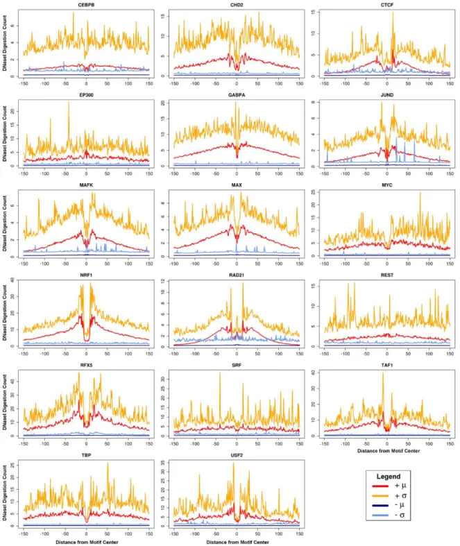
Aggregate DNaseI digestion profiles do not capture motif site heterogeneity
Aggregate mean DNaseI digestion profiles summarize positional DNaseI cleavage
preferences at TFBSs. These profiles convey a single value at each position, thus they lack
information regarding the variability in DNaseI activity at a given position across sites. Raj et al.
showed that variation in DNaseI activity at TF-bound SP1 motif sites exceeded that expected under
a multinomial model of DNaseI digestion signal [51]. To evaluate this more broadly, I determined
positional variability in DNaseI digestion signal for multiple TFs (Figures 2.2A and 2.3). I stratified
motif sites into active and inactive based on presence of corresponding ChIP-seq signal for the
factor in the same cell type. I used these to evaluate two common assumptions held by several
footprinting methods: 1) active TFBSs possess a general footprint pattern of local depletion in
DNaseI digestion relative to flanking regions; and 2) inactive motif sites contain approximately
uniformly distributed DNaseI digestion signal. For most factors, aggregate profiles for active sites
clearly produced expected DNaseI digestion patterns, but with relatively large standard deviations.
An investigation of individual binding sites clearly shows how sites deviate from the aggregate
pattern (Figures 2.2C and 2.2D). In some cases, the previously characterized sequence preferences
for DNaseI digestion [63] are visually apparent. For a minority of the TFs, the aggregate profile for
active sites portrays a visually weak footprint or none at all (i.e. SRF, Figure 2.3). Overall, TFs
exhibit aggregate profiles with consistently high coefficients of variation (Figure 2.4).
In spite of position-specific variability across motif sites, it is possible that DNaseI signal at
individual sites resemble the aggregate profile in shape but not scale. To quantify the similarity of
21
correlation coefficients between the aggregate profiles and every individual TFBS profile for
CEBPB, CHD2, and NRF1 (Figure 2.5). Among the 3 TFs, 30-63% of the individual profiles did not
correlate with the same class aggregate profile (Pearson’s r < 0.1). Interestingly, I found that 17-51% of individual profiles from the active and inactive classes exhibited stronger positive
correlations with the aggregate profile from the opposite class.
To further assess within and between class heterogeneity, I computed Pearson correlations
between the top 2000 individual DNaseI digestion profiles, ranked based on the number of
DNase-seq reads in a 100 bp window centered on the motif site, in the active and inactive classes for all
three factors. I observed small clusters of highly correlated sites, implying possible subgroupings
for DNaseI cleavage profiles within each class. I also found 34-53% of motif sites within each class
exhibited negative or no correlation to each other (Pearson’s r < 0) (Figures 2.2D and 2.6). Notably,
4-6% of correlations between sites from opposite classes had Pearson’s r > 0.5. These analyses of variability in DNaseI digestion signal strongly indicate that aggregate mean profiles do not
sufficiently capture the heterogeneity in DNaseI activity across motif sites.
We hypothesized that high correlations between sites from one class to the aggregate
profile of the opposite class may be partially attributed to similarities in binding preferences for
multiple TFs. Therefore, a motif site deemed inactive for a specific TF based on ChIP-seq data could
be active for another TF with a similar motif. I assessed this by determining how many inactive
motif sites overlapped ChIP-seq peaks for at least one other TF for each of 18 TFs in the K562 cell
line. I found that this was the case for 8.85% of all inactive sites (Figure 2.7). For most TFs, the
number of inactive motif sites was significantly larger than the number of active sites (Table 2.4).
Thus, while the number of inactive sites overlapping another ChIP-seq peak was relatively small,
these represented 0.41 to 32.21 times the total number of active motif sites for a TF. Footprint
patterns at inactive sites that resemble active sites due to the binding of another factor highlights
22
the accuracy of footprint predictions. This also applies to de novo footprinting as it becomes an
issue when annotating called footprints using motifs. A potential solution would be to exclude all
motif sites overlapping ChIP-seq peaks for multiple TFs. However, this would remove 66%-100% of
active sites for a TF. Additionally, this would require conducting a multitude of ChIP-seq
experiments and disregards the fact that many TFs have binding partners.
Modeling data heterogeneity for footprinting
To account for the high variance in DNaseI activity at motif sites, I devised a novel
supervised learning based footprint prediction framework called DeFCoM (Detecting Footprints
Containing Motifs). DeFCoM trains an SVM using extracted features from DNaseI digestion profiles
of motif sites labeled as active or inactive. In the training phase, DeFCoM applies a model selection
procedure to choose between a linear kernel and nonlinear RBF kernel (Figure 2.8; see Materials &
Methods). This allows DeFCoM to capture the complexity of the data when necessary with the RBF
kernel, while avoiding over-fitting, a common problem in supervised learning, by choosing the
linear kernel when that complexity is lacking. Once trained, the SVM uses features from DNaseI
digestion profiles for new, unlabeled motif sites to determine which are active and inactive in
another cell type/condition.
To assess DeFCoM’s classification accuracy, I first performed 5-fold nested cross validation
on 71 evaluation sets comprised of data from 18 transcription factors in the human cell-lines
GM12878, H1-hESC, HepG2, and K562 generated by the ENCODE project. Secondly, I tested
DeFCoM’s ability to generalize across cell types by training models using data from one cell type
and testing on an independent cell type. I also wanted to know whether using the RBF kernel
increased accuracy given the demonstrated heterogeneity in these data. Therefore, for both sets of
experiments, I used a linear and an RBF SVM and compared their classification performance. I will
23
operating characteristic (ROC) Area Under the Curve (AUC) values using all the data and also partial
AUC (pAUC) values corresponding to partial ROC curves at a 5% false positive rate (FPR) cutoff.
When applied to the 71 data sets, DeFCoM-RBF performed better than a random classifier in
all cases (Figure 2.9A). Notably, I observed a wide distribution of pAUC scores ranging from 0.096
to 0.981, but there was less variability in the full AUC scores (0.714-0.998). For the cross cell-line
experiments, I expected that additional variability across the two data sets would decrease
performance compared to the within cell-line cross validation tests. Indeed, I witnessed overall
lower scores from the former but by a marginal amount (median pAUC decrease of 0.021)
indicating there exist consistent footprint signals across cell types.
To determine whether using the nonlinear RBF kernel to model heterogeneity was
warranted, I repeated the above experiments using the linear kernel. Overall, DeFCoM-RBF
improved classification accuracy for all cell-lines in both experimental setups except for the cross
cell-line case where the test set was derived from data in the K562 cell line (Figure 2.9B). I saw that
the pAUC increased as much as 0.141 when using DeFCoM-RBF. However, the pAUC was essentially
the same in 31% of cross validation tests and 41% of cross cell-line tests. This demonstrates that
the RBF kernel can provide large gains in accuracy, but some factors or data sets may not possess
enough DNaseI signal heterogeneity to benefit from more complex footprint modeling.
Interestingly, DeFCoM-linear performed substantially better on cross cell-line tests when
training with GM12878 and evaluating with K562 data. This demonstrated the need for flexibility in
model complexity. Therefore, I incorporated a model selection step during DeFCoM training to
automatically determine the most appropriate kernel for a given test (see Materials & Methods). I
found that with the exception of CTCF, my model selection procedure identified the better model in
all cases in which there was a measurable difference between kernels (pAUC difference > 0.05;
24
DeFCoM and found the aforementioned approach produced the best results. Nevertheless, I
describe the alternative procedures in the following section.
Variations for DeFCoM training in cross cell-line applications
To address the decrease in classification accuracy of DeFCoM when training in one cell-line
and testing in another, I initially explored two methods in addition to the SVM model selection
procedure.
Mitigating Data set Shift
Given the variety of factors involved in generating DNase-seq and ATAC-seq data as well as
biological variability in the samples processed for sequencing, I considered the possibility that the
DNase-seq and ATAC-seq data used for training DeFCoM may differ enough from the data being
used during the classification phase of cross cell-line analyses to negatively impact classification
performance. More formally, I hypothesized that the joint distribution between inputs into
DeFCoM’s RBF kernel SVM and the outputs produced by this SVM differed between the training and
testing stage. This phenomena is more generally referred to in machine learning literature as data
set shift [64].
To account for the possibility of data set shift, I trained a logistic regression model with data
from GM12878 and K562 to obtain for each sample the probability that the sample was derived
from GM12878, P(GM12878), and the probability that it was derived from K562, P(K562). If more
than 25,000 motif sites existed in the active and inactive motif site sets for both cell-lines, I
randomly selected 25,000 samples from each of the active and inactive motif site sets, totaling to
100,000 sites. These samples were converted into feature vectors, and assigned the class label
“GM12878” or “K562”. The labeled feature vectors were then used to train an L2-regularized
logistic regression model. The regression model was then applied to feature vector representations
25
GM12878 motif sites were then filtered to include only those for which P(K562) ≥ 0.4. These
filtered motif sites were then used to train an RBF kernel SVM using 5-fold cross validation. Sample
weights were included for the SVM training such that training samples more similar to the K562
test samples would receive a greater weight. I defined the weight to be P(K562)/P(GM12878).
Table 2.5 provides the results of applying data set shift correction to DeFCoM for 17 transcription
factors.
Sequencing Depth Matching
Another consideration related to cross cell-line analyses is the difference in sequencing
depth between the training and testing set affecting DeFCoM performance. When the training data
set comes from DNase-seq/ATAC-seq data with a lower sequencing depth than the test data, the
dynamic range of DNaseI digestion frequencies at motif sites has the potential to be greater in the
test set. Arguably, this could create another scenario where data set shift is a concern. Although I
incorporate a square root transformation of the DNaseI digestion frequencies into the DeFCoM
framework to mitigate dynamic range issues, I also tested if matching the sequencing depths
between the training and testing data would improve DeFCoM’s classification accuracy.
Using the subsampling feature in SAMTools (Li et al., 2009), I down-sampled the K562
DNase-seq data to match the GM12878 DNase-seq data sequencing depth. I then used the GM12878
and K562 data to generate the training and test set feature vectors respectively. With the GM12878
feature vectors I used 5-fold cross validation to train the RBF kernel SVM of DeFCoM, and I applied
the trained model to the feature vector representations of the down-sampled K562 samples. Table
2.5 provides the results of this evaluation for 17 transcription factors. Compared to the model
selection procedure, both the data set shift correction and down-sampling approaches produced
26 Multiple variables impact motif-centric footprinting
In addition to addressing the heterogeneity of DNaseI signal at motif sites, my analyses
provide insights into some variables that may affect motif-centered footprinting performance,
though this is certainly not an exhaustive list of contributing factors. My observations suggest that
the “footprintability” i.e., the quality of footprinting, of any particular data set is a function of
several characteristics. I noted that features of the data from a particular cell-line and the specific
TF being considered can contribute to footprintability. For instance, the pAUC is 0.36 higher on
average in K562 compared to HepG2 for all cross validation experiments (Figure 2.9), suggesting
that footprint signals in K562 are better overall. Within GM12878, the cross validation pAUC scores
across TFs range from 0.210 to 0.915, highlighting the variability in footprintability across TFs.
Lastly, pAUCs for CHD2 are higher than CEBPB in all cell types (Figure 2.11), suggesting active
footprints for some factors are in general easier to discriminate than for others.
It is important to note that the four cell lines I use span a wide range of sequencing depths
(Table 2.6). I wondered how closely footprintability was associated with total sequencing depth.
Since the signal quality across data sets can widely vary, I also wondered whether the “effective”
sequencing depth, based on the number of reads in DNaseI hypersensitive sites, was more
important than simply the raw sequencing depth. I used mean pAUC values from DeFCoM’s nested
cross validation experiments for each TF across all cell lines to compare footprintability based on
total and effective sequencing-depth. Overall, I found that for most factors, accuracy increased
nonlinearly with respect to total sequencing depth, but not effective sequencing depth (Figure
2.12).
To better understand the trade-off between sequencing depth and signal quality, I focused
on data from GM12878 and H1-hESC since they possess very different signal-to-noise ratios (0.19
versus 0.43 FRiP score). I performed 5-fold nested cross validation using DeFCoM and data from