A Robust and Higher Precision Time Delay Estimation Method Facing Low Signal to Noise Ratio Conditions

(1)

http://www.sciencepublishinggroup.com/j/ijiis doi: 10.11648/j.ijiis.20180703.12

ISSN: 2328-7675 (Print); ISSN: 2328-7683 (Online)

A Robust and Higher Precision Time Delay Estimation

Method Facing Low Signal to Noise Ratio Conditions

Junhao Li

1

, Wenhong Liu

2, *

, Niansheng Chen

2

, Guangyu Fan

2

1

School of Electrical Engineering, Shanghai Dianji University, Shanghai, China 2_{School of Electronic Information, Shanghai Dianji University, Shanghai, China}

Email address:

*

Corresponding author

To cite this article:

Junhao Li, Wenhong Liu, Niansheng Chen, Guangyu Fan. A Robust and Higher Precision Time Delay Estimation Method Facing Low Signal to Noise Ratio Conditions. International Journal of Intelligent Information Systems. Vol. 7, No. 3, 2018, pp. 28-37.

doi: 10.11648/j.ijiis.20180703.12

Received: October 27, 2018; Accepted: December 30, 2018; Published: December 12, 2018

Abstract:

Many available signals in the real world are usually weak with impulse noises and/or outliers, and we also need to have higher estimation precision in applications. Our focus of attention is pretty much on integrating robustness and accuracy under lower signal to noise ratio (SNR) with impulse noises. Although traditional fractional adaptive time delay estimation (TDE) methods have higher precision, the results of estimation are unreasonable when the signals contain some impulse noises. While, most proposed robust algorithms later can work well mainly with high SNR. In this paper, considering the practical problem in equipment fault acoustic localization based on TDE methods, an improved robust fractional adaptive time delay estimation method is addressed facing lower SNR conditions. First, the impulse noises are modeled as Alpha stable distribution, and the integer part of TDE is getting by using covariate correlation approach. Then, the integer estimation value is used as initial parameter value of time delay. Covariant sequence is the input of time delay estimator. Next, fractional TDE value is adaptive obtained by iteration under minimum average p norm criterion. Covariant sequence weakens irrelevant noises, meanwhile preserves time delay information between original sequences. Computer simulations and comparative experiments show that improved method has better estimation results. This method is robust and higher precision, and especially under impulse environment and low SNR conditions.

Keywords:

Equipment Acoustic Fault Location, Adaptive Fractional Time Delay Estimation, Lower Signal to Noise Ratio, Robust

1. Introduction

There are many methods for fault diagnosis of electromechanical equipment. Fault sound location can use sound field information and array processing technology determine sound source position, intuitively find fault source, then find out cause of fault, such as air conditioning compressor abnormal sound positioning [1], wind turbine aerodynamic noise source location [2], and gearbox noise control [3]. Sound source localization system is micro, independent and portable. Large equipment detection system can be supplemented by sound source localization technology according some faulty has sound feature [4]. In sound source localization based on time delay estimation, Performance of

(2)

weighting algorithm based on quadratic correlation, which has good applicability under strong noise and reverberation. Literature [9] compares correlation, covariation and fractional low-order covariance algorithms and proves fractional lower-order algorithm is the more robust. Literature [10] proposed covariation correlation algorithm to suppress impulse noise, estimation accuracy is higher than covariation method and correlation method under low SNR. Correlation method can only estimate integer bits of time delay estimation value, when locating some low-frequency fault sound sources [11]. If sampling frequency only satisfies sampling theorem, fractional bit error has a great influence on positioning. Correlation peak is not sharp when sampling rate increases, it is difficult to find peak position, at the same time, increasing sampling rate increases the difficulty in hardware implementation.

There are two ways to improve estimation resolution. One is interpolation; the other is to directly estimate non-integer delay. Literature [12] uses correlation method estimate time delay value firstly, then uses sinc function process one of two input signals for getting a certain percentage sampling period time delay, performs correlation operation to compare with previous peak for more accurate time delay estimates; repeating this process on previous basis can improve estimation effect, but resolution is still affected. Literature [13] proposes ETDGE algorithm, which proves that the least squares of the estimator reaches the lower bound of Cramer. Literature [14] improved ETDE algorithm to verify performance of color input and low SNR case algorithms. Literature [15] use time delay estimation method measure power station boilers high temperature, Based on background noise is very close to Gaussian process, in order to overcome difficulty of estimating precise time delay in power plant boiler under low time-varying SNR, An explicit time delay gain estimation algorithm based on fourth-order cumulant is studied. Literature [16] proposes a non-integer adaptive time delay estimation method based on minimum mean p-norm, it is called LMPFTDE algorithm and has good robustness in both Gaussian noise and impulse noise environments, algorithm cost function is multimodal, cost function is unimodal when delay value is between D−0.5 and D+0.5 (D is delay true value). Other algorithms need to calculate an accurate integer bit estimate as an iterative initial value of LMPFTDE to estimate non-integer delay true value.

Under sampling satisfies sampling theorem, considering low signal-to-noise ratio of fault signal and noise characteristics of containing pulse signal, this paper gets a more accurate time delay estimation value through two steps. Firstly, observation sequence is processed to self-covariation and covariation, correlation processes self-covariation and covariation get integer estimation value as initial value of non-integer adaptive time delay estimation algorithm. Then, two covariation sequence is used as input signal of LMPFTDE algorithm to achieve a more accurate estimation value at a low sampling rate.

2. Alpha Stable Distribution and

Covariation

2.1. Alpha Stable Distribution

α

stable distribution is a generalized Gaussian model [17], According to generalized central limit theorem, it is the only type of limit distribution that constitutes the sum of independent and identically distributed random variables, Gaussian distribution is its subclass. The difference between Gaussian distribution and

α

stable distribution is that Gaussian distribution has an exponential tail and

α

stable distribution has an algebraic tail,

α

stable distribution can better describe pulse process in noise.

With a few exceptions,

α

stable distribution probability density function has not analytical expression. Characteristic function and probability density function are mutually uniquely determine relationship, characteristic function is essentially inverse Fourier transform of probability density function, which can fully describe statistical properties of random distribution. The following is a description of characteristic function of

α

stable distribution.

If random variable has parameters 0 < α ≤ 2, γ ≥ 0, −1 ≤ β ≤ 1. ɑ feature function has following expression [17]_:

∅ = exp {jɑt − γ| | [1 + jβsgn t ω t, α ]}, (1)

ω t, α = #tan %

& ，α ≠ 1

&

%log|t|，α = 1

, (2)

sgn t =* 1 ，t > 0

0，t = 0

−1，t < 0

, (3)

Then random variable X obeys

α

stable distribution. In equation (1), parameter

α

is characteristic index, which determines degree of impulsiveness of

α

stable distribution, the smaller value, the thicker distribution tail, and the more pronounced pulse in sample. On the contrary, the value becomes larger, corresponding distribution tail becomes thinner, and pulse in sample is weakened.

α

=

2

,

α

stable distribution corresponds to Gaussian distribution,

α

stable distribution is a generalized Gaussian distribution. Parameter

β

determines distribution slope,

γ

is dispersion coefficient, which is a dispersion degree measure of sample relative to mean, and ɑ is positional parameter, corresponding to median or mean of

α

stable distribution.

2.2. Covariation

Covariation [18] is a fractional lower order statistics (FLOS). In SαS distribution random variables (symmetric

α

stable distribution), it is similar to covariance in Gaussian distribution random variables. Two joint distribution random variables

x

and

y

satisfying SαS, covariation is defined.

[,, -] = . /0〈 23〉_{5 67}

(3)

In equation (4), S represents unit circle; represents a spectral measure of a SαS distribution random vector (

x

,

y

), 9〈:〉= |9|〈:〉sign（Z）. Due spectral measure µ(。) is

not easy to obtain, in practice, covariation is obtained by the Fractional lower order moment (FLOM). Two joint SαS

distributed random variables

x

and

y

satisfying

2

1 <

α

≤

, they have the following relationship.

[X, Y]?=@ AB

〈CDE〉

@ |B|C FG, 1≤ p< α, (5)

In equation (5), F_Gis dispersion coefficient of random variable

y

. Some properties of covariation play an important role in

α

stable signal processing and analysis. Property 1 Covariation [X,Y]α is linear to the first argument

x

, if

x

₁, 2

x

and y obey union SαS, [ AX1 + BX2, Y] = A[ X1, Y] + B[ X2, Y] , (6)

In formula (6), A and B are arbitrary real numbers. Property 2 If

y

₁and

y

₂ are independent,

x

、 1

y

和 2

y

obey union

_S

α

_S

, then [X, AY3+ BY&]?=AJ 2 3K [X, Y3] + BJ 2 3K [ X, Y&] , (7)

In formula (7), A and B are arbitrary real numbers. Property 3 If

x

and

y

are independent and subject to joint SαS, then[ X, Y] = 0. When α = 2,

x

and

y

obey joint Gaussian distribution of zero mean, covariation of

x

and

y

degenerates into covariance. [ X, Y] = E(XY), (8)

3. Algorithm Analysis

3.1. Noise Model Assume two received signals /₃(n) and /_&(n) satisfy following discrete signal model: /3(n)= s(n)+L3(n), (9)

/&(n)= λs(n- D)+L&(n), (10)

λs(n- D) is the delayed source signal relative to s(n), λ is the attenuation factor (usually λ= 1), v₃(n) v_&(n) are background noise received by two receivers respectively, obeying

α

stable distribution. It is assumed that signal and noise, noise and noise are statistically independent. 3.2. Covariation Correlation Algorithm Covariation [/₃ N , /_& N ]_O23 and self-covariation [/3 N , /3 N ]O23 can be written as [/3 N , /& N ]O23 = [7 N + L3 N , 7 N − P + L& N ]O23 = [7 N , 7 N − P ]O23+ [Q N , L3 N ]O23 +[L3 N , 7 N − P ]O23+ [L3 N , L& N ]O23, (11) [/3 N , /3 N ]O23 = [7 N + L3 N , 7 N + L3 N ]O23 = [7 N , 7 N ]O23+ [Q N , L3 N ]O23 +[L3 N , 7 N ]O23+ [L3 N , L3 N ]O23, (12)

signal and noise are assumed to be statistically independent, depending on the nature of the covariation, [Q N , L3 N ]O23 = 0, (13)

[L3 N , 7 N − P ]O23= 0, (14)

[v3 n , v& n ]R-3= 0, (15)

[L3 N , 7 N ]O23 = 0, (16)

[L3 N , L3 N ]O23= TUV N . (17)

Equations (10) and (11) can be reduced to [/3 N , /& N ]O23= [7 N , 7 N − P ]O23, (18)

[/3 N , /3 N ]O23= [7 N , 7 N ]O23+ [L3N , L3 N ]O23 (19) covariation of /₃ N and /_& N is W_X3& Y , self-covariation of /₃ N is W_X33 Y WX3& Y = E{x3 N [/& N + Y ]}〈R23〉 = E{7 N [7 N − P + Y ]}〈R23〉 = WU[[ Y + P), (20)

WX33 Y = E{x3 N [/3 N + Y ]}〈R23〉 = E{7 N [7 N + Y ] + v3 N [L3 N + Y ]}〈R23〉 = WU[[ Y + TUV Y , (21)

Original sequences are processed by self-covariation and covariation, self-covariation series can be regarded as covariation series is shifted and added with an interference, covariation series preserves phase information of original

sequence and weakens irrelevant noise, increases

signal-to-noise ratio, suppress impulse noise, but in the case of limited data processing, interference noise will not be zero.

Correlation time delay estimation effect of

covariant-processed raw data is better than direct correlation and covariation methods in the same signal-to-noise ratio and pulse environment.

3.3. LMPFTDE Algorithm

(4)

estimation. Output error e(n) is at time n.

e n /3 N \] N /3^N P_ N `

/3 N \] N ∑def2d7bNc b P_ N !/3 N b!, (22)

\] N is the gain estimate, sinc（k）≜ 8jk %l

%l , the goal is

to minimize average p-norm of error, p-th order moment of error is the smallest, and cost function of algorithm is

J ≜ E |n n |:_! _{f \] n , P_ n !}_{, (23)}

This is a two-dimensional nonlinear optimization problem. Relaxation method is used to transform decoupling into two one-dimensional optimization problems, gain and time delay are respectively iterated to obtain optimal solution. Within certain time delay range, cost function J is a unimodal with a unique minimum, steepest descent method and gradient technique are used, statistical average is replaced by instantaneous value of error signal. Adaptive iterative formula is

\] n 1 \] n 5_p q__p]r!

\] n 5ps|e n | O

s\] n

\] n t5p|n N |O237\N n N ! ∑def2d7bNc b P_ N ! /3 N b!, (24)

P_ n 1 P_ n 5u q_u_r!

P_ n 5us|e n | O

sP_ n

P_ n t5u|n N |O237\N n N ! ∑def2dv b P_ N ! /3 N b!, (25)

f k Xw8 xy 2[ezU y_y ，

µ

_g,

D

µ

are convergence factors, taking a small positive number,

1 <

p

≤

2

. In order to improve stability and convergence speed of algorithm, normalization is performed.

\] n 1 \] n _‖|3

E‖CC}t5p|n N |

O23_{7\N n N ! ∑}d _{7bNc b} _{P_ N !}

ef2d /3 N b!~, (26)

P_ n 1 P_ n _‖|3

E‖CC}t5u|n N |

O23_{7\N n N ! ∑}d _{v b} _{P_ N !}

ef2d /3 N b!~, (27)

‖x3‖OO /3 N • O /3N • 1 O ⋯ /3 N • O, (28)

Cost function E |n n |O" contains sinc function, it is multi-peak, it can be treated as a single peak by limiting range of initial value.

3.4. Improved Non-integer Adaptive Time Delay Estimation Algorithm

In this paper, two received signals, /3(n), /&(n) are

processed to get covariation sequence and self-covariation sequence. covariation series preserves phase information of original sequence and weakens irrelevant noise, increases signal-to-noise ratio, suppress impulse noise. covariation series length is doubled and more iterations can be performed. More iterative value references can make delay estimate

closer to the true value. Then, WX3&, WX33 regard as

equivalent time series as input signals of LMPFTDE algorithm, cost function of LMPFTDE algorithm is multi-peak function, iterative algorithm may not converge directly, when iteration value is between D−0.5 and D+0.5 (D is time delay true value), cost function is unimodal. So correlation time delay estimation is used to estimate time delay integer bit for Rc21 and Rc11, obtained estimation value

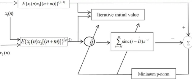
is used as initial value of LMPFTDE algorithm. Finally, adaptive time delay estimation is performed to obtain higher resolution time delay estimate. Block diagram of improved non-integer adaptive time delay estimation algorithm is shown in Figure 1.

Figure 1. Block diagram of improved fractional adaptive time delay estimation method.

4. Computer Simulation Experiments

Computer simulation experiment is used to compare

(5)

signal and noise model, source S(n) of band-limited flat spectrum is generated by Gaussian white noise through 6-order Butterworth low-pass filter with bandwidth of 0.2, impulse noise is obeyed by α stable distribution. Mixed signal-to-noise ratio MSNR= 10lg(•_[&/F_‚) [16] is set,

σ

S2

represents source signal variance,

γ

_v represents noise dispersion coefficient, signal length n=10000, and delayed signal s(n-D) is generated by 61-order FIR filter of

∑d 7bNc[b − P]

ef2d 92e, true value is D=3.2

T

S , initial value is 3

T

_S . Covariation sequence length is 20000, the following results are averages of 50 independent experiments.

Experiment 1 Under the same α value and MSNR condition, p=1.1, =1.5, MSNR=0 dB, LMPFTDE algorithm and improved algorithm iteration step are both 0.09. Observe LMPFTDE algorithm and improved algorithm convergence curve, as shown in Figure 2 and Figure 3.

Figure 2. Convergence curve of LMPFTDE algorithm.

Figure 3. Convergence curve of the improved algorithm.

Table 1. Performance comparison on LMPFTDE algorithm and improved algorithm.

LMPFTDE algorithm mproved algorithm

Root mean square error 0.09182 0.05220

Estimated value (median) 3.1191 3.1543

In LMPFTDE algorithm and improved time delay estimation algorithm, length of input signal indicates number of algorithm can be iterated. LMPFTDE algorithm input signal length is 10000, the maximum number of iterations can be 10000. The improved algorithm input signal is 20000, and the maximum number of iterations that can be 20000.

From Figure 2, Figure 3 and Table 1, LMPFTDE algorithm can converge to near true value, and improved algorithm can converge to true value and fluctuate around true value. Iterative delay value median is used as delay estimation value.

Compare with LMPFTDE algorithm, estimation value of improved algorithm is closer to delay true value, and root mean square error of improved algorithm is smaller than LMPFTDE algorithm.

Experiment 2 compares estimation accuracy between LMPFTDE algorithm and improved algorithm under same

value and different MSNR conditions.

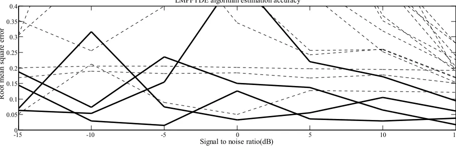
α

=1.5, MSNR

changes from -15 dB to 15 dB at 5 dB intervals. Root mean square error of the two algorithm estimates is shown in Figure 4 and Figure 5.

0 1000 2000 3000 4000 5000 6000 7000 8000 9000 10000 2.95

3 3.05 3.1 3.15 3.2 3.25

Iterations number

E

s

tim

a

te

d

e

la

y

v

a

lu

e

(T

)

LMPFTDE algorithm convergence curve

0 0.2 0.4 0.6 0.8 1 1.2 1.4 1.6 1.8 2 x 104 2.95

3 3.05 3.1 3.15 3.2 3.25

Iterations number

E

s

tim

a

te

d

e

la

y

v

a

lu

e

(

T

)

(6)

Experimental conditions: p=1.1, delay convergence factor and signal-to-noise ratio iteration step are equal parameters, parameters change from 0.01 to 0.69 of 18 parameters at

intervals of 0.04, results obtained for each set of parameters are represented by lines.

(a) Comparison of algorithm estimation performance under different parameters

(b) Different parameter sets estimate performance

Figure 4. LMPFTDE algorithm estimation accuracy (α=1.5).

-150 -10 -5 0 5 10 15

0.05 0.1 0.15 0.2 0.25 0.3 0.35 0.4

LMPFTDE algorithm estimation accuracy

Signal to noise ratio(dB)

R

o

t

m

ea

n

s

q

u

a

re

e

rr

o

r

-15 -10

-5

0 2

4 6

8 10

12 14

16 18

10-2 10-1 100 101

Parameter group

R

o

t

m

ea

n

s

q

u

ar

e

er

ro

r

-150 -10 -5 0 5 10 15

0.05 0.1 0.15 0.2 0.25 0.3 0.35 0.4

Improved algorithm estimation accuracy

Signal to noise ratio(dB)

R

o

t

m

ea

n

s

q

u

ar

e

er

ro

(7)

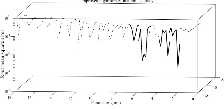
Figure 5. Improved algorithm estimation accuracy (α=1.5).

Figure 4 and Figure 5 are root mean square error results of LMPFTDE algorithm and improved algorithm simulation of 18 sets parameters respectively. In Figure 4(a) and Figure 5(a), in single broken line, the lowest mean square error of improved algorithm from -5 dB to 5 dB is lower than the lowest mean square error of LMPFTDE algorithm, iteration step size and signal to noise ratio are 0.21. Under different SNR, the minimum root mean square error of improved algorithm is lower than the LMPFTDE algorithm, but it is not on a polyline. In Figure 4(b) and Figure 5(b), estimation performance of improved algorithm is better than LMPFTDE algorithm overall. Algorithm parameter has a great influence on performance. It is better to choose appropriate parameters in different environments. Under this experimental condition, the best parameters are within the parameter interval.

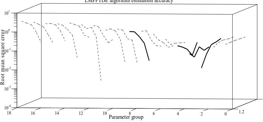
Experiment 3 compares estimation accuracy between LMPFTDE algorithm and improved algorithm under same

MSNR and different α conditions. MSNR=0 dB, α

changes from 1.2 to 2 at 0.2 intervals. Root mean square error of two algorithm estimates is shown in Figure 6 and Figure 7. (Experiment 3 conditions are the same as Experiment 2).

Figure 6 and Figure 7 are root mean square error results of LMPFTDE algorithm and improved algorithm by 18 sets parameters respectively. In Figure 6(a) and Figure 7(a), the lowest mean square error of improved algorithm is lower than the lowest mean square error of LMPFTDE algorithm. Lower root mean square error of improved algorithm is on the same line over entire interval, delay step and signal-to-noise ratio iteration step are 0.33. In Figure 6(b) and Figure 7(b), performance of improved algorithm is better than LMPFTDE algorithm over all. Algorithm parameter has a great influence on performance. It is better to choose appropriate parameters in different environments. Under this experimental condition, the best parameters are within the parameter interval.

-15 -10

-5

0 2

4 6

8 10

12 14

16 18

10-4 10-3 10-2 10-1 100

Parameter group

R

o

t

m

ea

n

s

q

u

ar

e

er

ro

r

1.2 1.4 1.6 1.8 2

0 0.05 0.1 0.15 0.2 0.25 0.3 0.35 0.4

Alpha

R

o

t

m

ea

n

s

q

u

ar

e

er

ro

(8)

Figure 6. LMPFTDE algorithm estimation accuracy (MSNR=0 dB).

Figure 7. Improved algorithm Estimation accuracy (MSNR=0 dB).

1.2 0 2

4 6

8 10

12 14

16 18

10-4 10-3 10-2 10-1 100 101

Parameter group

R

o

t

m

ea

n

s

q

u

ar

e

er

ro

r

1.2 1.4 1.6 1.8 2

0 0.05 0.1 0.15 0.2 0.25 0.3 0.35

0.4 Improved algorithm estimation accuracy

Alpha

R

o

t

m

e

a

n

s

q

u

a

re

e

rr

o

r

1.2 0 2

4 6

8 10

12 14

16 18

10-3 10-2 10-1 100

Parameter group

R

o

t

m

ea

n

s

q

u

ar

e

er

ro

(9)

5. Conclusions

Covariation correlation algorithm is suitable for processing low SNR signals, and has a good suppression effect on impulse noise. It can accurately estimate delay value integer bits. Original signal is processed by covariation, then covariation sequence are used as input of LMPFTDE algorithm, input signal length is doubled, more iterations can be performed, delay estimation value is closer

to real value, uncorrelated noise is eliminated,

signal-to-noise ratio is improved, original signal phase information is preserved. Time delay estimation obtained by covariation correlation algorithm is used as initial value of LMPFTDE algorithm, finally non-integer delay estimation value is obtained. Non-integer adaptive time delay estimation algorithm is also a cross-correlation algorithm in principle, and processing performance of wideband signal is better than narrow band.

Experiment 1 compares convergence process and estimation results of two algorithms and analyzes advantages of improved algorithm. Experiment 2 simulates different SNRs and experiments two algorithms. Results show that improved algorithm is better than the LMPFTDE algorithm and the parameters of improved algorithm are given. Experiment 3 simulates noise of different pulse environments, compares root mean square error estimated by LMPFTDE algorithm and improved algorithm, and obtains a set parameters that improved algorithm has a good estimation effect in the whole interval.

In this paper, time delay estimation values of two algorithms are selected as follows: median of all iteration values as delay estimation value. In order to obtain a more accurate delay estimation value, delay estimation value can be: observation convergence curve, median of iterative value after convergence, that can improve the estimation accuracy. LMPFTDE algorithm limits iteration initial value in a certain range. Within this range, delay estimation cost function is a unimodal, using variable step size method makes adaptive convergence process steady-state fluctuation smaller and have faster convergence, need not consider convergence to a local optimal solution.

Acknowledgements

This work was partly supported by Chinese National Natural Science Funding Project (No. 61172108), and Shanghai Dianji University Horizontal Research Cooperation Project (No. 17B56). The authors would also like to express their deep appreciation to Professor Tianshuang Qiu and the Dalian University of Technology.

References

[1] Qian Shie. Acoustic camera——Making our community more quiet [J]. Foreign Electronic Measurement Technology, 2009, 28 (2): 5-8.

[2] Ottermo F, Möllerström E, Nordborg A, et al. Location of aerodynamic noise sources from a 200 kW vertical-axis wind turbine [J]. Journal of Sound & Vibration, 2017, 400: 154-166. [3] Shi Quan, Guo Dong, Shi Xiaohui, et al. Study on noise source localization of transmission based on microphone array [J]. Journal ofVibration and Shock, 2012, 31 (13): 134-137. [4] Xie D, Wang M, Zhu J Q, et al. An equipment fault sound

location system design [J]. Applied Mechanics & Materials, 2014, 462-463 (462-463): 298-301.

[5] Li J H, Liu W H. Characteristics analysis and modeling of fault sound and background noise of large central air conditioner [J]. Journal of Electrical and Electronic Engineering, 2018, 6 (1): 30-35.

[6] Liu Min, Zeng Yumin, Zhang Ming, et al. Improved algorithm for time delay estimation of speech signal based on quadratic correlation [J]. Journal of Applied Acoustics, 2016, 35 (3): 255-264.

[7] Zhang Q, Zhang L. An improved delay algorithm based on generalized cross correlation [C]//Information Technology and Mechatronics Engineering Conference, IEEE, 2017: 395-399. [8] Shen Guoqing, Yang Jiedong, Chen Dong, Liu Weilong, Zhang

Shiping, An Chain. Study on temperature estimation of boiler acoustic temperature measurement based on quadratic correlation PHAT-β algorithm [J]. Journal of Power Engineering, 2018, 38 (08): 617-623.

[9] Li J H, Liu W H. Performance comparison on three time delay estimation algorithms using experiments, communications [J]. Electrical & Computer Science, 2017, 5 (3): 24-28.

[10] Liu W, Wang Y, Qiu T. Evoked potential latency delay estimation by using covariation correlation approach [C]//International Conference on Bioinformatics and Biomedical Engineering, IEEE, 2008: 652-655.

[11] Sun X, Liu Y, Zhang J, et al. Measurement and analysis of a horizontal-axis washing machine for low-frequency abnormal noise [C]. 2016 13th International Conference on Ubiquitous Robots and Ambient Intelligence (URAI), Xi'an, 2016: 735-739.

[12] Jiang Xue, Liu Yuanyuan, Lei Weijia, et al. FPGA implementation of a cross-correlation delay estimator with low SNR [J]. Telecommunication Engineering, 2014, 54 (7): 951-957.

[13] So H C, Ching P C. Performance analysis of ETDGE-an efficient and unbiased TDOA estimator [J]. IEE Proceedings - Radar Sonar and Navigation, 1998, 145 (6): 325-330.

[14] W. Xia, W. Jiang and L. Zhu, "An Adaptive Time Delay Estimator Based on ETDE Algorithm with Noisy Measurements," in Chinese Journal of Electronics, vol. 26, no. 4, pp. 760-767, 7 2017.

[15] Yang X, Liu X, Shen J. The research of the explicit time delay and gain estimation algorithm based on fourth-order cumulants in acoustic pyrometry in the power plant boiler [C]//Chinese Automation Congress, 2017: 6091-6097.

(10)

[17] Nikias C L, Shao M. Signal processing with Alpha-stable distributions [M]. New York: John Wiley & Sons Inc, 1995.