CONFIDENCE INTERVALS FOR STOCHASTIC VARIATIONAL INEQUALITES
Michael Lamm
A dissertation submitted to the faculty of the University of North Carolina at Chapel Hill in partial fulfillment of the requirements for the degree of Doctor of
Philosophy in the Department of Statistics and Operations Research.
Chapel Hill 2015
Approved by: Shu Lu
ABSTRACT
MICHAEL LAMM: Confidence intervals for solutions to stochastic variational inequalities (Under the direction of Shu Lu)
This dissertation examines the effects of uncertain data on a general class of optimization and equilibrium problems. The common framework used for modeling these problems is a stochastic variational inequality. Variational inequalities can be used to model conditions that characterize an equilibrium state, or describe necessary conditions for solutions to constrained optimization problems. For example, Cournot-Nash equilibrium problems and the Karush-Kuhn-Tucker conditions for nonlinear programming problems both fit in the framework of a variational inequality. Uncertain model data can be incorporated into a variational inequality through the use of an expectation function. A variational inequality defined in this manner is referred to as a stochastic variational inequality (SVI).
ACKNOWLEDGEMENTS
First and foremost I must recognize my advisor Shu Lu. It has been a pleasure learning from and working with you. If not for the time and effort you have invested in me I would not be at this point. While I cannot fully express my gratitude for all that you have done in this space, I hope the work in this dissertation is able to provide some reflection of its effects. Next, I must thank Professor Amarjit Budhiraja. I have benefited greatly from the time I have had to work with you, and your impact on me and this dissertation are greatly appreciated.
I would also like to recognize the members of my dissertation committee, Professors Vidyadhar Kulkarni, Gabor Pataki, and Scott Proven, along with the other instructors I have had at UNC, Professors Nilay Argon, Edward Carlstein, Vladas Pipiras, and Serhan Ziya. All of you have been wonderful and have made my time as a graduate student a truly rewarding experience that has exceeded all of my expectations. Also, I would like to thank Alison Kieber and the rest of the staff in the STOR department for helping to keep me blissfully unaware of all of the administrative work that must have accompanied my time as a graduate student.
To my fellow students here at UNC, in particular those in my cohort and Sean Skwerer, thank you for all of your support. Your advice, input, and willingness to be sounding boards for everything from teaching, research, practice talks, and avoiding work has always been appreciated. I feel very lucky to have overlapped with all of you here in the STOR department and wish all of you the best moving forward.
TABLE OF CONTENTS
LIST OF TABLES . . . ix
LIST OF FIGURES. . . x
LIST OF ABBREVIATIONS AND SYMBOLS . . . xi
1 Introduction . . . 1
1.1 Stochastic variational inequalities . . . 4
1.2 Piecewise affine functions . . . 6
1.3 Background . . . 9
1.4 Outline . . . 20
2 Simultaneous confidence intervals . . . 22
2.1 Construction simultaneous confidence intervals . . . 22
2.2 Application to a stochastic Cournot-Nash equilibrium problem . . . 26
3 Confidence intervals for the normal map solution . . . 37
3.1 Introduction . . . 37
3.2 The first method . . . 39
3.3 The second method . . . 46
3.4 Interval computation . . . 52
3.5 Numerical examples . . . 58
3.5.1 Example 1 . . . 59
3.5.2 Example 2 . . . 61
3.5.3 Example 3 . . . 63
4 Direct confidence intervals . . . 67
4.2 Methodology . . . 70
4.3 Numerical examples . . . 75
4.3.1 Example 1 . . . 76
4.3.2 Example 2 . . . 78
5 Relaxed confidence intervals . . . 80
5.1 Introduction . . . 80
5.2 Methodology . . . 81
5.3 Numerical example . . . 89
LIST OF TABLES
2.1 Producer parameter values. . . 28
2.2 Values for price elasticityeand demand D. . . 28
2.3 Reference prices p0 and demands q0 . . . 29
2.4 Time period parameters in base price demand function . . . 29
2.5 Coverage rates of confidence regions forz0,α=.05 . . . 32
2.6 Coverage rates of simultaneous confidence intervals for z0,α=.05 . . . 33
2.7 Half-widths of intervals for (z0)59,α=.05 . . . 34
2.8 Coverage rates of simultaneous confidence intervals for x0,α=.05 . . . 36
3.1 Coverage rates (z0)1 α=.05 . . . 59
3.2 Coverage rates (z0)2, α=.05 . . . 59
3.3 Coverage rates of (z0)2 and half-widths for (z0)2 by cone, N = 2,000 . . . 60
3.4 Coverage rates for (z0)3. . . 62
3.5 Ratios of upper bounds to interval half-widths . . . 63
3.6 Coverage rates for (z0)j,N = 100 andN = 3,000,α=.05 . . . 65
4.1 Coverage rates for (x0)j,N = 100 andN = 3,000, α=.05 . . . 77
4.2 Coverage rates of (x0)i,α=.05 . . . 78
4.3 Intervals for (x0)i by cone,N = 2,000,α=.05 . . . 79
5.1 Coverage rates for (z0)j,N = 100 andN = 2,000,α1=α2 =.025 . . . 90
LIST OF FIGURES
LIST OF ABBREVIATIONS AND SYMBOLS
SAA SVI ar(·) C1(X,Rn) ηα
j(·,·) ˜ ηα2
j (·,·) fSnor hα
j(·,·,·) ˜
hα2
j (·,·,·) K(z) ΠS N NS(x) Rn ri(S) TS(x) w
N,j
xN x0 zN z0
Sample average approximation Stochastic variational inequality
Width of an individual confidence interval for (z0)j using the first method The space of continuously differentiable mappingsf :X→Rn
Width of an individual confidence interval for (z0)j for the second method Width of a relaxed individual confidence interval for (z0)j
The normal map induced byf and S
Width of an individual confidence interval for (x0)j Width of a relaxed individual confidence interval for (x0)j The critical cone toS atz
The Euclidian projector onto a setS Sample size
The normal cone toS atx
Set ofn dimensional real valued vectors The relative interior of a convex setS The tangent cone toS atx
Width ofjth component of a simultaneous confidence interval for (z0)j A solution to an SAA problem
A solution to an SVI
CHAPTER 1
Introduction
Variational inequalities model a general class of equilibrium problems and also arise as first-order necessary conditions of optimization problem, see (Attouch et al., 2009; Facchinei and Pang, 2003; Ferris and Pang, 1997a,b; Giannessi and Maugeri, 1995; Giannessi et al., 2001; Harker and Pang, 1990; Pang and Ralph, 2009). A variational inequality, defined formally in§1.1, is characterized by a setSand a functionf. In many problems of interest, data defining the function are subject to uncertainty. One way to handle such uncertainty is to treatf as an expectation function, and this gives rise to a stochastic variational inequality (SVI). For many problems the expectation function lacks a closed form expression and a numerical approximation is generally required. Such approximations usually make use of some sampling procedure. Based on how sampling is incorporated into the approximation scheme, SVI algorithms can be classified into stochastic approximation (SA) methods and sample average approximation (SAA) methods. SA methods as introduced in (Robbins and Monro, 1951) update iterate points with samples taken at each step. The application of SA methods to SVIs have been studied in (Chen et al., 2014; Jiang and Huifu, 2008; Juditsky et al., 2011; Koshal et al., 2013; Nemirovski et al., 2009a) and references therein. For the development of SA methods in stochastic optimization, see (Nemirovski et al., 2009b; Polyak, 1990; Polyak and Juditsky, 1992) and references therein.
(G¨urkan et al., 1999; King and Rockafellar, 1993; Shapiro et al., 2009). Xu (Xu, 2010) showed the convergence of SAA solutions to the set of true solutions in probability at an exponential rate under some assumptions on the moment generating functions of certain random variables; related results on the exponential convergence rate are given in (Shapiro and Xu, 2008). Working with the exponential rate of convergence of SAA solutions, Anitescu and Petra in (Anitescu and Petra, 2011) developed confidence intervals for the optimal value of stochastic programming problems using bootstrapping. Limiting distributions for SAA solutions were obtained in (King and Rockafellar, 1993, Theorem 2.7) and (Shapiro et al., 2009, Section 5.2.2). For random approximations to deterministic optimization problems, universal confidence sets for the true solution set were developed by Vogel in (Vogel, 2008) using concentration of measure results.
The major contribution of this dissertation is the development methods for the efficient calculation of confidence intervals for the true solution to an SVI from a single SAA solution, based on the asymptotic distribution of SAA solutions. To our knowledge, the computation of confidence sets for an SVI’s solution based upon the asymptotic distribution of SAA solutions started from the dissertation of Demir (Demir, 2000). By considering the normal map formulation (to be defined formally in§1.1) of variational inequalities, Demir used the asymptotic distribution to obtain an expression for confidence regions of the solution to the normal map formulation of an SVI. Because some quantities in that expression depend on the true solutions and are not computable, Demir proposed a substitution method to make that expression computable. He did not, however, justify why that substitution method preserves the weak convergence property needed for the asymptotic exactness of the confidence regions. Standard techniques for the required justification cannot be used due to the general nonsmooth structure of S and the discontinuities this creates in certain quantities.
expo-nential rate of convergence, and involved calculating a weighted-sum of a family of functions. The method was later simplified by Lu in (Lu, 2012) by using a single function from the family. Due to the potentially piecewise linear structure that underlies the asymptotic dis-tribution of SAA solutions, the methods in (Lu, 2012; Lu and Budhiraja, 2013) may require working with piecewise linear transformations of normal random vectors. Lu in (Lu, 2014) proposed a different method to construct asymptotically exact confidence regions, by using only the asymptotic distribution and not the exponential convergence rate. The method in (Lu, 2014) is easier to use since it has the advantage of working (with high probability) with linear transformations of normal random vectors, even when the asymptotic distribution of zN is not normal.
Component-wise confidence intervals for the true solution are generally easier to visu-alize and interpret compared to confidence regions. By finding the axis-aligned minimal bounding box of a confidence region of z0 (or x0), one can find simultaneous confidence intervals that jointly contain z0 (or x0) with a probability no less than a prescribed con-fidence level. Additionally, individual concon-fidence intervals provide a quantitative measure of the uncertainty in each individual component, and therefore cary important information not covered by larger confidence sets. Individual confidence intervals that can be obtained by using confidence regions are too conservative for any practical use, especially for large scale problems. A method to construct individual confidence intervals for z0 using linear estimates was analyzed in (Lu, 2014). While computationally efficient, the method requires some restrictive assumptions to guarantee that the specified level of confidence is met.
andx0are related by the equalityx0= ΠS(z0). From a confidence set ofz0, one can obtain a confidence set forx0, by projecting the confidence set ofz0 ontoS. The resulting set will coverx0 with a rate at least as large as the coverage rate of the original confidence set for z0. WhenS is a box, individual confidence intervals of x0 can be obtained from projecting the individual confidence intervals ofz0 ontoS. We shall refer to such approaches as “indi-rect approaches.” The indi“indi-rect approaches are convenient to implement when the setS is a box, or has a similar structure that facilitates taking (individual) projections. Beyond those situations, it would be hard to use the indirect approaches for finding confidence intervals forx0.
In Section 1.1 the SVI and SAA problems are formally defined along with their normal map formulations. Pertinent properties of piecewise affine functions are reviewed in §1.2 along with the notion of B-differentiability. Previous works on the relationship between the SVI and SAA problems are summarized in §1.3, and §1.4 outlines the methods for interval computation discussed in remainder of this dissertation.
1.1 Stochastic variational inequalities
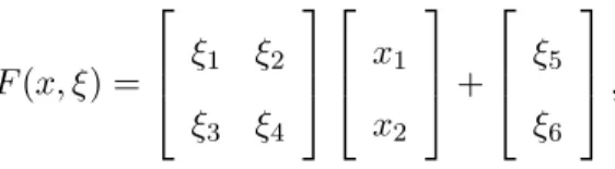
An SVI is defined as follows. Let (Ω,F, P) be a probability space, andξ be a random vector defined on Ω and supported on a closed subset Ξ ofRd. LetO be an open subset ofRn, and F be a measurable function from O×Ξ to Rn, such thatEkF(x, ξ)k<∞ for each x∈O. LetS be a polyhedral convex set inRn. The SVI problem is to find a pointx∈S∩O such that
0∈f0(x) +NS(x), (1.1)
wheref0(x) =E[F(x, ξ)] andNS(x)⊂Rn denotes the normal cone toS atx:
NS(x) ={v∈Rn|hv, s−xi ≤0 for eachs∈S}.
Here h·,·idenotes the scalar product of two vectors of the same dimension.
method takes independent and identically distributed (i.i.d) random variablesξ1, ξ2, . . . , ξN with the same distribution as ξ and constructs a sample average function. The sample average function fN :O×Ω→Rnis defined by
fN(x, ω) =N−1 N X
i=1
F(x, ξi(ω)). (1.2)
The SAA problem is to find a pointx∈O∩S such that
0∈fN(x, ω) +NS(x). (1.3)
Solutions of (1.1) are referred to as true solutions, whereas solutions of (1.3) are refereed to as SAA solutions.
The formulations of the SVI and SAA problems as given in (1.1) and (1.3) involve the set valued mapping NS(·). In their normal map formulations the set valued mapping is removed and solutions are identified as the zeros of single-valued non-smooth functions. For the SVI, the function is the normal map induced by f0 and S, f0nor,S : Π
−1
S (O) → Rn, defined as
f0nor,S(z) =f0◦ΠS(z) + (z−ΠS(z)). (1.4)
Here ΠS denotes the Euclidian projector onto the set S, Π−S1(O) is the set of all points z ∈ Rn such that ΠS(z) ∈ O, and f
0◦ΠS is the composite function of f0 and ΠS. The normal map formulation of (1.1) is to find a pointz∈Π−1
S (O) such that
f0nor,S(z) = 0. (1.5)
The two formulations are related by the fact thatx∈O∩S solves (1.1) only ifz=x−f0(x) satisfies (1.5). Moreover when this equality is satisfied it additionally holds that ΠS(z) =x.
The normal map induced byfN and S is similarly defined on Π−S1(O) to be
The normal map formulation of the SAA problem is then to find z∈Π−S1(O) such that
fN,Snor(z) = 0, (1.7)
where (1.7) and (1.3) are related in the same manner as (1.5) and (1.1). In general, for a function G mapping from a subset D of Rn back into Rn, the normal map induced by G and S is a map defined on Π−S1(D) with GSnor(z) =G◦ΠS(z) +z−ΠS(z).
By assumption, S is a polyhedral convex set, so the Euclidian projector ΠS is a piece-wise affine function. In the next section we provide a summary of pertinent properties of piecewise affine functions, in particular the notion of B-differentiability.
1.2 Piecewise affine functions
A continuous function f : Rn → Rm is piecewise affine if there exists a finite col-lection of affine functions fj, j = 1, . . . , l, such that for all x ∈ Rn the inclusion f(x) ∈ {f1(x), . . . , fl(x)} holds. The affine functions fj are refereed to as the selection functions off. When eachfj is a linear function f is called piecewise linear.
Closely related to piecewise affine functions is the concept of a polyhedral subdivision. A polyhedral subdivision of Rn is defined to be a finite collection of convex polyhedra, Γ ={P1, . . . , Pl}, satisfying the following three conditions:
1. Each Pi is of dimensionn.
2. The union of all the Pi is Rn.
3. The intersection of any two Pi and Pj, 1≤ i6=j ≤l, is either empty or a common proper face of both Pi and Pj.
We next consider the special case of the Euclidian projector onto a polyhedral convex set S, a thorough discussion of which can be found in (Scholtes, 2012, Section 2.4). LetFbe the finite collection of all nonempty faces of S. On the relative interior of each nonempty face F ∈ F the normal cone toS is a constant cone, denoted as NS(riF), and the set addition CF =F +NS(riF) results in a polyhedral convex set of dimension n. The collection of all such sets CF form the polyhedral subdivision of Rn corresponding to ΠS. This collection of sets is also referred to as the normal manifold of S, with each CF called an n-cell in the normal manifold. Each k-dimensional face of an n-cell is called a k-cell in the normal manifold for k= 0,1, . . . , n. The relative interiors of all cells in the normal manifold of S form a partition ofRn.
Next we introduce the concept of B-differentiability. A function h :Rn → Rm is said to be B-differentiable at a point x ∈ Rn if there exists a positive homogeneous function, H:Rn→Rm, such that
h(x+v) =h(x) +H(v) +o(v).
Recall that a functionH is positive homogeneous ifH(λx) =λH(x) for all positive numbers λ∈Rand points x∈Rn. The function H is referred to as the B-derivative ofh atx and will be denoted dh(x). When dh(x) is also linear, dh(x) is the classic Fr´echet derivative (F-derivative).
A piecewise affine functionf, while not F-differentiable at all points, is B-differentiable everywhere. More precisely, let Γ be the polyhedral subdivision associated with f. At points x in the interior of a polyhedron Pi ∈Γ, df(x) is a linear function equal to dfi(x), the F-derivative of the corresponding selection functionfi. When x lies in the intersection of two or more polyhedra, let Γ(x) = {Pi∈Γ|x∈Pi}, I = {i|Pi∈Γ(x)} and Γ0(x) = {Ki = cone(Pi−x)|i∈I}. That is, Γ(x) is the collection of elements in Γ that contain x, and Γ0(x) is the “globalization” of Γ(x) along with a shift of the origin. With this notation, df(x) is piecewise linear with the family of selection functions given by {dfi(x)|i∈I} and the corresponding conical subdivision given by Γ0(x).
to be
TS(x) ={v∈Rn|there existst >0 such thatx+tv∈S},
and the critical cone to S at a point z∈Rn to be
K(z) =TS(ΠS(z))∩ {z−ΠS(z)}⊥.
As shown in (Robinson, 1991, Corollary 4.5) and (Pang, 1990, Lemma 5), for any point z∈Rn and any sufficiently small h∈Rn the equality
ΠS(z+h) = ΠS(z) + ΠK(z)(h) (1.8)
holds, which implies
dΠS(z) = ΠK(z). (1.9)
The connection to the normal manifold ofSfollows from the fact that for all pointszin the relative interior of ak-cell the critical coneK(z) is a constant cone; see (Lu and Budhiraja, 2013, Theorem 8), and thusdΠZ(z)(·) is the same function for allz in the relative interior of a k-cell. For points z and z0 in the relative interior of different k-cells dΠS(z)(·) and dΠS(z0)(·) can be quite different, and as a result small changes in the choice ofzcan result in significant changes in the form ofdΠS(z)(·).
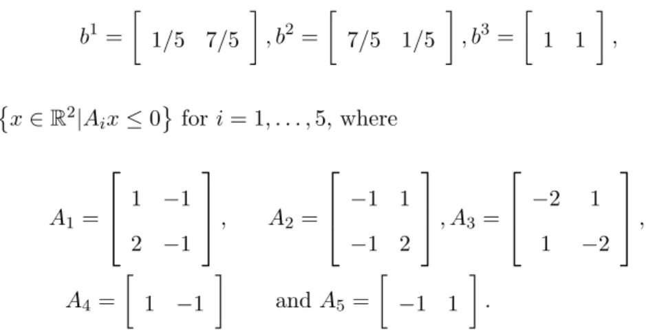
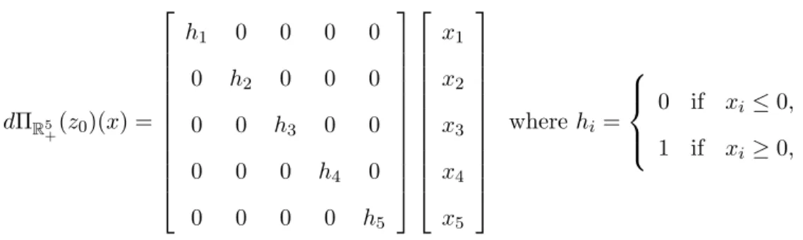
To illustrate these concepts we end this section with an example. Take S = R2
+, where R+ = {x∈R, x≥0}. The set S has four nonempty faces with F =
R2
+, R+× {0}, {0} × {0}, {0} ×R+ . The corresponding 2-cells in the normal manifold of S are the orthants R2
+,R+×R−,R−2 and R−×R+. There are five k-cells with k < n. Four 1-cells are the half-lines defined by the positive and negative axes,R+×{0},{0}×R+, R−× {0},{0} ×R−, and the fifthk-cell with k= 0 is the origin{0} × {0}.
The restriction of ΠS to each 2-cell is a linear function, with the functions represented by the matrices
1 0 0 1
,
1 0 0 0
,
0 0 0 0
and
0 0 0 1
At x= (0,1)∈ri ({0} ×R+), ΠS is not F-differentiable but has B-derivative dΠS(x)(·)
dΠs(x)(h) =
v 0 0 1
h1 h2
where v=
1 if h1 ≥0, 0 if h1 ≤0.
In contrast, for a pointx0 = (,1)∈ri R2 +
for >0, the B-derivativedΠS(x0)(·) is a linear function represented by the identity matrix.
1.3 Background
In this section we discuss previous work on the computation of confidence sets for the true solution to an SVI. This section begins with a review of conditions under which the SAA solutions will have the required asymptotic properties. These properties include the almost sure convergence of the SAA solutions to a true solution, an exponential rate for the convergence in probability, and the weak convergence of SAA solutions.
The following notation will be used throughout this section and the remainder of this dissertation. Letx0 and xN denote solutions to the true SVI and SAA problems (1.1) and (1.3). We use Σ0 to denote the covariance matrix ofF(x0, ξ), and ΣN to denote the sample covariance matrix of{F(xN, ξi)}N
i=1. A normal random vector with meanµand covariance matrix Σ shall be denoted by N(µ,Σ). A χ2 random variable with l degrees of freedom will be denoted byχ2
l. Weak convergence of random variables Yn toY will be denoted as Yn ⇒Y.
Assumption 1. (a) EkF(x, ξ)k2 <∞ for allx∈O.
(b) The map x 7→ F(x, ξ(ω)) is continuously differentiable on O for a.e. ω ∈ Ω, and
EkdxF(x, ξ)k2 <∞ for all x∈O.
(c) There exists a square integrable random variable C such that for all x, x0 ∈O
kF(x, ξ(ω))−F(x0, ξ(ω))k+kdxF(x, ξ(ω))−dxF(x0, ξ(ω))k ≤C(ω)kx−x0k,
From Assumption 1 it follows that f0 is continuously differentiable on O, see, e.g., (Shapiro et al., 2009, Theorem 7.44). For any nonempty compact subset X of O, let C1(X,Rn) be the Banach space of continuously differentiable mappings f : X → Rn, equipped with the norm
kfk1,X = sup x∈Xk
f(x)k+ sup x∈Xk
df(x)k. (1.10)
Then in addition to providing nice integrability properties for fN, as shown in (Shapiro et al., 2009, Theorem 7.48) Assumption 1 will guarantee the almost sure convergence of the sample average approximation function fN tof0 as an element of C1(X,Rn) and that df0(x) =E[dxF(x, ξ)].
Assumption 2. Suppose that x0 solves the variational inequality (1.1). Let z0 = x0 − f0(x0), L=df0(x0),K0 =TS(x0)∩ {z0−x0}⊥, and assume thatLnorK0 is a homeomorphism from Rn toRn, where LnorK
0 is the normal map induced by L and K0.
Assumption 2 guarantees that x0 is a locally unique solution and that (1.1) has a locally unique solution under sufficiently small perturbations of f0 in C1(X,Rn), see (Lu and Budhiraja, 2013, Lemma 1) and the original result in (Robinson, 1995). Since the critical cone K0 is a polyhedral convex cone, LnorK0 is a piecewise linear function. It was
shown in (Robinson, 1992) that LnorK
0 is a homeomorphism if and only if the determinants
of the matrices representing its selections functions all have the same nonzero sign. Shorter proof of this result can be found in (Ralph, 1994) and (Scholtes, 1996). A piecewise linear function with this property is said to be coherently oriented. A special case in which the coherent orientation condition holds is when the restriction of L on the linear span of K0 is positive definite. In particular, iff0 is strongly monotone onO, then the entire matrixL is positive definite and LnorK
0 is a global homeomorphism. Another special case is when the
coneK0 =Rn+, the nonnegative orthant; for such a case the coherent orientation condition on LnorK
0 is equivalent to the requirement that Lis a P-matrix.
The normal maps LnorK
0 and f nor
1, the chain rule of B-differentiability implies that f0nor,S is differentiable, with its B-derivative atz0 given by
df0nor,S(z0)(h) =df0(x0)◦dΠS(z0)(h) +h−dΠS(z0)(h) (1.11)
with corresponding conical subdivision Γ0(z0).
Applying (1.9) toz0, one can see the normal mapLnorK0 is exactlydf0nor,S(z0), a result that first appeared in (Robinson, 1992). Note that the B-derivative for the normal map fN,Snor, denoted by dfN,Snor(·), will take an analogous form to (1.11).
The following theorem is adapted from (Lu and Budhiraja, 2013, Theorem 7). It pro-vides the almost sure and weak convergence of the SAA solutionszN andxN. Those results are obtained by combining convergence properties of the sample average functionfN with sensitivity analysis techniques originally developed in (Robinson, 1995) for deterministic variational inequalities. Similar results were also shown in (King and Rockafellar, 1993, Theorem 2.7) using the concept of subinvertibility and a set of assumptions that are im-plied by those used here.
Theorem 1. Suppose that Assumptions 1 and 2 hold. Let Y0 be a normal random vector
in Rn with zero mean and covariance matrix Σ0. Then there exist neighborhoodsX0 of x0
and Z of z0 such that the following hold. For almost every ω ∈ Ω, there exists an integer Nω, such that for each N ≥Nω, the equation (1.7) has a unique solutionzN in Z, and the variational inequality (1.3) has a unique solution in X0 given by xN = ΠS(zN). Moreover,
lim
N→∞zN =z0 andNlim→∞xN =x0 almost surely,
√
N(zN −z0)⇒(LnorK0)
−1(Y
0), (1.12)
√
N LnorK0 (zN−z0)⇒Y0, (1.13)
and
√
N(ΠS(zN)−ΠS(z0))⇒ΠK0 ◦(L
nor K0)
−1(Y
The results of Theorem 1 follow from the convergence of fN to f0 in C1(X,Rn), and the existence of locally unique solutions to (1.1) for sufficiently small perturbations off0 in this same space. In particular, Assumptions 1 provides a sufficient conditions for the weak convergence of √N(fN −f0) in C1(X,Rn) which combined with Assumption 2 yields the asymptotic distributions in (1.12), (1.13) and (1.14).
In his dissertation (Demir, 2000), Demir developed methods to compute confidence regions for true solutions of SVIs using (1.13). Recognizing that the resulting expression depended on the true solution through both Σ0 and LnorK0, he proposed to use ΣN and
dfN,Snor(zN) in the expression for the confidence regions. He did not, however, justify how such a replacement preserves the weak convergence property needed for the asymptotic exactness of the confidence regions. The discontinuity of dΠS(z) with respect to z, and in particular the fact thatdΠS(zN) does not in general converge todΠS(z0), prevents standard techniques from being applicable for such a justification. The issue that arises is that when dΠS(z0) is piecewise linear the probability of dΠS(zN) being a linear map goes to one as the sample size N goes to infinity; see (Lu, 2014, Proposition 3.5). While this poses a challenge for establishing the exactness of confidence regions constructed using dfN,Snor(zN) as an estimate for LnorK
0, it also illustrates the desirability of using such regions since their
expression would with high probability involve only linear functions.
To establish the exactness of confidence regions constructed usingdfN,Snor(zN) Lu in (Lu, 2014, Theorem 3.3 and 4.1) examined the relationship between df0nor,S(z0)(zN −z0) and −dfN,Snor(zN)(z0−zN) and proved the following results.
Theorem 2. Suppose that Assumptions 1 and 2 hold. Then for each >0 we have
lim N→∞Pr{
√
Nkdf0nor,S(z0)(zN −z0) +dfN,Snor(zN)(z0−zN)k> }= 0. (1.15)
Consequently, we have
Moreover, if Σ0 is nonsingular, then
−√NΣ−N1/2dfN,Snor(zN)(z0−zN)⇒ N(0, In). (1.17)
If Σ0 is singular, let ρ > 0 be the minimum of all positive eigenvalues of Σ0, and let l be
the number of positive eigenvalues of Σ0 counted with regard to their algebraic multiplicity.
DecomposeΣN as
ΣN =UNT∆NUN
where UN is an orthogonal n×n matrix, and ∆N is a diagonal matrix with monotonically
decreasing elements. Let DN be the upper-left submatrix of ∆N whose diagonal elements
are at least ρ/2. Let lN be the number of rows in DN, (UN)1 be the submatrix of UN that
consists of its firstlN rows, and (UN)2 be the submatrix that consists of the remaining rows
ofUN. Then for almost everyω the equalitylN =lholds for sufficiently largeN. Moreover,
N
dfN,Snor(zN)(z0−zN) T
(UN)T1D−N1(UN)1
dfN,Snor(zN)(z0−zN)
⇒χ2
l (1.18)
and
N dfN,Snor(zN)(z0−zN)T(UN)T2(UN)2dfN,Snor(zN)(z0−zN)⇒0. (1.19)
Using (1.17), (1.18) and (1.19) we can give computable expressions for asymptotically exact confidence regions for z0. To this end, for anyα ∈ (0,1) and integer k let χ2k(α) be the (1−α) percentile of a χ2 random variable with k degree’s of freedom, and let k · k
∞
denote the ∞-norm for a vectorx ∈Rn. Then for any >0 and integer N we define sets RN when ΣN is nonsingular, andRN, when ΣN is singular, to be
RN = n
z∈Rn N
dfN,Snor(zN)(z−zN) T
Σ−N1
dfN,Snor(zN)(z−zN)
≤χ2 n(α) o , (1.20) RN,=
z∈Rn N
dfN,Snor(zN)(z−zN) T
(UN)T1D −1 N (UN)1
dfN,Snor(zN)(z−zN)
≤χ2 lN(α)
k√N(UN)2dfN,Snor(zN)(z−zN)k∞≤
Depending on if ΣN is singular or not, by Theorem 2 we will have that either
lim
N→∞Pr{z0 ∈RN}= 1−α or limN→∞Pr{z0 ∈RN,}= 1−α.
Note that the expression for confidence regions in the nonsingular case is the same as that proposed by Demir. Since the nonsingular case can be treated as a specialization of the singular case with lN = n and = 0, moving forward we focus on the singular case and consider regionsRN,.
While the regions RN, have a specified asymptotic level of confidence, they are not necessarily amenable to easy interpretation and visualization. It was thus suggested in (Lu, 2014) to construct easier to interpret simultaneous confidence intervals by finding the axis-aligned minimal bounding box that contains the region RN,. We examine questions raised by this approach to building simultaneous confidence intervals in an application to a stochastic Cournot-Nash equilibrium problem of moderate size in Chapter 2.
We now move our focus to the question of computing individual confidence intervals for components of z0. A first approach would be to use the component interval of the simultaneous confidence intervals considered above, but such intervals are too conservative for any practical use. In (Lu, 2014) a natural expression for individual confidence intervals suggested by (1.17) was analyzed. Recall that (1.17) required the additional assumption that Σ0 be nonsingular. Since this assumption is used throughout the discussion of individual confidence intervals we formally declare it as
Assumption 3. Let Σ0 denote the covariance matrix of F(x0, ξ). Suppose that the
deter-minant of Σ0 is strictly positive.
properties of ΣN as well as the locations of F(xN, ξi), i = 1, . . . , N, with respect to the normal manifold of S.
Before summarizing the results for the confidence intervals suggested by (1.17) some notation must be introduced. Let df0nor,S(z0) be piecewise linear with l pieces and the cor-responding conical subdivision {K1, . . . , Kl} .Then df0nor,S(z0)|Ki =Mi for each i= 1, . . . , l,
where Mi stands for the matrix that represents df0nor,S(z0) on Ki. Under Assumption 2, df0nor,S(z0) is a global homeomorphism so each matrix Mi is invertible. We then define Yi = M−1
i Y0. Since Y0 is a multivariate normal random vector each Yi is a multivariate normal random vector with covariance matrixMi−1Σ0Mi−T.
We define the number
rji = q
(Mi−1Σ0Mi−T)jj
for each i= 1, . . . , l andj = 1, . . . , n. Then for each α∈(0,1) it follows that
Pr
|(Yi)j| ≤rij q
χ2 1(α)
= 1−α.
With this notation the following theorem was shown in (Lu, 2014, Theorem 5.1)
Theorem 3. Suppose that Assumptions 1, 2 and 3 hold. LetKi, Mi, Yiandri
j be defined as
above. For each integerN withd(fN)S(zN) being an invertible linear map, define a number
rN j = q
dfnor
N,S(zN)−1ΣNdfN,Snor(zN)−T)jj
for each j= 1, . . . , n. Then for each real numberα∈(0,1)and for each j= 1, . . . , n,
lim N→∞Pr
√
N|(zn−z0)j| rN j ≤
q χ2 1(α) ! = l X i=1 Pr (Yi)
j ri j ≤ q χ2
1(α) and Yi ∈Ki
! (1.21)
Moreover, suppose for a given j= 1, . . . , n that the following equality
Pr
(Yi) j ri j ≤ q χ2
1(α) and Yi ∈Ki
! = Pr
(Yi) j ri j ≤ q χ2 1(α) !
holds for each i= 1, . . . , l. Then for each real number α∈(0,1),
lim
N→∞Pr |(zN−z0)j| ≤
p χ2
1(α)rN j √
N !
= 1−α.
We see in (1.21) that this method of constructing individual confidence intervals, while easily computable using only the sample data, produces intervals whose asymptotic level of confidence is dependent on the true solution, unless the condition below (1.21) is satisfied. The latter condition is satisfied, whendf0nor,S(z0) is a linear function or has only two selection functions, in which case the intervals computed from this method will be asymptotically exact. However, in general the level of confidence for such intervals cannot be guaranteed. The issue with the linear estimate dfN,Snor(zN) is that it does not properly account for the possibly piecewise linear structure ofdf0nor,S(z0). This limitation motivates the development of the methods proposed in Chapter 3 and 4. The three methods all produce intervals that maintain their desired asymptotic properties in the general setting by using estimates that capture the possibly piecewise linear structure ofdf0nor,S(z0). To construct such estimates we will need the following additional assumption.
Assumption 4. (a) For each t∈Rn and x∈X, let
Mx(t) =E[exp{ht, F(x, ξ)−f0(x)i}]
be the moment generating function of the random variable F(x, ξ)−f0(x). Assume
1. There exists ζ > 0 such that Mx(t) ≤ exp
ζ2ktk2/2 for every x ∈ X and every t∈Rn.
2. There exists a nonnegative random variable κ such that
kF(x, ξ(ω))−F(x0, ξ(ω))k ≤κ(ω)kx−x0k
for allx, x0 ∈O and almost every ω∈Ω.
(b) For each T ∈Rn×n andx∈X, let
Mx(T) =E[exp{hT, dxF(x, ξ)−df0(x)i}]
be the moment generating function of the random variable dxF(x, ξ)−df0(x). Assume
1. There exists ς > 0 such that Mx(T) ≤ exp
ς2kTk2/2 for every x ∈ X and every T ∈Rn×n.
2. There exists a nonnegative random variable ν such that
kdxF(x, ξ(ω))−dxF(x0, ξ(ω))k ≤ν(ω)kx−x0k
for allx, x0 ∈O and almost every ω∈Ω.
3. The moment generating function of ν is finite valued in a neighborhood of zero.
First note that when Assumption 4 holds the conditions of Assumption 1 are satisfied. From Assumption 4 it follows thatfN converges tof0in probability at an exponential rate, as shown in (Lu and Budhiraja, 2013, Theorem 4) based on a general result (Shapiro et al., 2009, Theorem 7.67). That is, there exist positive real numbers β1, µ1, M1 and σ1, such that the following holds for each >0 andN:
Pr (kfN −f0k1,X ≥)≤β1exp{−N µ1}+ M1
n exp
−N 2
σ1
. (1.22)
Revisiting Theorem 1, if one additionally supposes that Assumption 4 holds, then as shown in (Lu and Budhiraja, 2013, Theorem 7), there exist positive real numbers 0, β0, µ0, M0 and σ0, such that the following holds for each ∈(0, 0] and eachN:
Pr (kxN−x0k< )≥Pr (kzN −z0k< )
(1.23) ≥1−β0exp{−N µ0} −
M0 n exp
−N 2
σ0
The convergence of SAA solutions to the set of true solutions in probability at an exponential rate was also shown using the concept of subinvertibility in (Xu, 2010) with an assumption similar to Assumption 4.
The exponential rate of convergence as given in (1.23) was used in (Lu and Budhiraja, 2013) to estimate df0nor,S(z0) by a weighted-sum of a family of functions. The estimates were later simplified in (Lu, 2012) by using a single function from the family. Due to the computational ease of using a single function we focus our presentation to the estimates for df0nor,S(z0) used in (Lu, 2012). In this approach a point nearzN is used in the estimate fordΠS(z0). More precisely, for each cell Ci in the normal manifold of S define a function di:Rn→Rby
di(z) =d(z, Ci) = min x∈Cik
x−zk, (1.24)
and a function Ψi :Rn→Rnby
Ψi(·) =dΠS(z)(·) for any z∈riCi. (1.25)
In (1.24) any norm for vectors inRncan be chosen, and in (1.25) anyz∈riCi can be chosen sincedΠS(z) is the same function on the relative interior of a cell. Next, choose a function g:N→R satisfying
1. g(N)>0 for eachN ∈N. 2. lim
N→∞g(N) =∞.
3. lim N→∞
N
g(N)2 =∞.
4. lim N→∞g(N)
nexpn−σ
0(g(NN))2
o
= 0 for σ0 = min
n
1 4σ0,
1 4σ1,
1 4σ0(E[C])2
o
, where σ0, and σ1 are as in (1.22) and (1.23) respectively and C as in Assumption 1.
5. lim N→∞
Nn/2
g(N)nexp
−σg(N)2 = 0 for each positive real number σ. Note thatg(N) =Np for any p∈(0,1/2) satisfies the above requirements.
Now for each integer N and any point z ∈Rn, choose an index i
0 by letting Ci0 be a
that contains zand di(z)≤1/g(N). Then define functions ΛN(z) :Rn→Rn by
ΛN(z)(h) = Ψi0(h), (1.26)
and ΦN : Π−S1(O)×Rn×Ω→Rn by
ΦN(z, h, ω) =dfN(ΠS(z))◦ΛN(z)(h) +h−ΛN(z)(h). (1.27)
Moving forward we will be interested in ΦN(zN(ω), h, ω), which for convenience we will express as ΦN(zN)(h) with the ω suppressed. We shall use zN∗ to denote a point in the relative interior of the cell Ci0 associated with (N, zN). With this notation it follows that
dΠS(zN∗) = Ψi0 and
ΦN(zN)(h) =dfN(ΠS(zN))◦dΠS(z∗N)(h) +h−dΠS(zN∗ )(h). (1.28)
We end the review of previous works with the following results shown in (Lu, 2012, Corollaries 3.2 and 3.3).
Theorem 4. Suppose that Assumptions 2 and 4 hold. For each N ∈N, letΛN and ΦN be as defined in (1.26) and (1.27). Then
lim
N→∞Pr [ΛN(zN)(h) =dΠS(z0)(h) for all h∈R
n] = 1, (1.29)
and there exists a positive real number θ, such that
lim N→∞Pr
" sup h∈Rn,h6=0
kΦN(zN)(h)−df0nor,S (z0)(h)k
khk <
θ g(N)
#
= 1. (1.30)
Moreover suppose Assumption 3 holds, and let ΣN be as defined above. Then
√
NΣ−01/2ΦN(zN)(zN −z0)⇒ N(0, In),
and
√
1.4 Outline
In the remainder of this dissertation we develop methods to compute confidence intervals for the true solution to an SVI, and apply those methods in stochastic optimization and equilibrium problems. In Chapter 2 we begin by examining the computation of simultaneous confidence intervals from the confidence regions given in (1.20) using the approach suggested in (Lu, 2014). Of particular interest will be the sensitivity of the interval widths and performance to the choice of the two parameters that arises in the case of a degenerate covariance matrix. The sensitivity of the interval’s width to the parameters is first examined through a discussion of the interval’s computation and the role of the parameters in these computations. The chapter then introduces the framework of stochastic Cournot-Nash equilibrium problems. The procedures for computing confidence regions and intervals are then applied to an example of the European gas market with numerical comparisons and sensitivity analysis results for both the confidence regions and intervals.
bounds for the interval lengths. The chapter ends with a comparison of the different methods using three numerical examples.
In Chapter 4 we propose a direct method for constructing individual confidence intervals for components of the true solution to an SVI as formulated in (1.1). The approaches for constructing confidence intervals for the normal map formulation of an SVI proposed in Chapter 3 cannot be applied to this problem due to the addition of a possibly noninvertible function to the asymptotic distribution. The new function also raises an issue unique to this chapter, namely, the possibility of components of the SAA solutions equaling the corresponding components of the true solution with a nonzero probability. This possibility provides a potential lower bound on the performance of any interval that contains the SAA solution, and therefore shifts the focus from asymptotically exact intervals to intervals for which a lower bound on the level of confidence can be guaranteed. A method for constructing intervals is then presented along with a theoretical justification. The chapter ends with two numerical examples.
CHAPTER 2
Simultaneous confidence intervals
2.1 Construction simultaneous confidence intervals
In this chapter we examine the computation and performance of confidence regions and simultaneous confidence intervals forz0. We focus on the case when the sample covariance matrix is singular, from which the nonsingular case can then be treated as a specialization. The singular case is of additional interest due to the dependence of the confidence regions on the choice of the parameter and valuelN. By Theorem 2, the confidence regions RN, in (1.20) are asymptotically exact for all > 0, but it remains to be seen how sensitive their performance is to the choice of for fixed sample sizes. For the choice of lN, recall thatlN determines the matricesDN, (UN)1, and (UN)2, and corresponds to the number of eigenvalues of ΣN that are treated as nonzero. In Theorem 2, the smallest eigenvalue of Σ0 is used to determine lN. In practice, since only sample data are available, lN and the matrices DN and (UN)1 must be determined in a different manner.
To begin, finding the left and right endpoints of the simultaneous confidence intervals requires solving
zr
j =maximum (z)j and zjl = minimum (z)j
z∈RN, z∈RN,
(2.1)
for j = 1,2. . . , n, where (z)j denotes the jth component of the vector z. If dfN,Snor(zN) is a piecewise linear function with corresponding conical subdivision {K1, . . . , Km}, then problems in (2.1) needs to be further broken down to the following problems
zi,jr =maximum (z)j and zi,jr = minimum (z)j z∈RN,∩Ki z∈RN,∩Ki
(2.2)
for j = 1,2. . . , n and i = 1, . . . , m, to account for the different expressions for dfN,Snor(zN) on each Ki. The right and left endpoints for the jth component interval are then zrj =
max i=1,...,mz
r
i,j andzjl = mini=1,...,mzi,jl .
Computation of the endpoints is greatly simplified whendfN,Snor(zN) is a linear function. In this case, the simultaneous confidence intervals are given by
(zN)1−wN, 1,(zN)1+wN,1
× · · · ×
(zN)n−wN,n,(zN)n+wN,n
(2.3)
wherew
N,j is the optimal value of the following problem:
maximize (w)j subject to N
dfN,Snor(zN)(w)T
(UN)T1D−N1(UN)1
dfN,Snor(zN)(w)
≤χ2lN(α) k√N(UN)2dfN,Snor(zN)(w)k∞≤.
(2.4)
Note that both lN and are responsible for determining the constraints in (2.4), the problem to find an interval’s endpoints. The first constraint in that problem
N
dfN,Snor(zN)(w)T
(UN)T1D−N1(UN)1
dfN,Snor(zN)(w)
≤χ2lN(α) (2.5)
defines an unbounded set wheneverlN is strictly less thann. With the linear independence between the rows of (UN)1 and (UN)2, the second constraint
k√N(UN)2dfN,Snor(zN)(w)k∞≤ (2.6)
complements the first constraint to yield a bounded feasible region and therefore a guaran-teed finite optimal solution to (2.4). In the following proposition we see thatw
N,j depends on as an affine function whose slope and intercept are determined bylN.
Proposition 1. Suppose that dfN,Snor(zN) is a linear homeomorphism andΣN has decompo-sitionΣN =UT
N∆NUN,where UN is an orthogonal matrix with rowsuN,1, . . . , uN,nand∆N
is a diagonal matrix with elements λ1 ≥λ2 ≥ · · · ≥λn. For a choice of lN with λlN >0, let DN be a diagonal matrix with elementsλ1, . . . , λlN,
(UN)1 =
uN,1
.. .
uN,lN
and (UN)2 =
uN,lN+1 .. . uN,n .
Then for each j= 1, . . . , n, the optimal value of (2.4) is an affine function of with
wN,j = s
χ2 lN(α)
PlN
i=1(cN,juTN,i)2λi
N + √ N n X
i=lN+1
|cN,juTN,i|, (2.7)
where cN,j is the jth row of dfN,Snor(zN)−1.
Proof. Let VN and TN be the subspaces spanned by n
uT
N,1, . . . , uTN,lN
o and n
uT
N,lN+1, . . . , u
T N,n
o
vectord(fN)S(zN)(w) can be decomposed as
dfN,Snor(zN)(w) =v+t
with v ∈ VN and t ∈ TN. Denoting the jth row of dfN,Snor(zN)−1 by cN,j, (2.4) can be reformulated as
maximize cN,jv+cN,jt
subject to N[vT(UN)T1DN−1(UN)1v]≤χ2lN(α)
k√N(UN)2tk∞≤
v∈VN, t∈TN.
(2.8)
By expressing v∈VN as v=PlN
i=1siuTN,i and t∈WN as t= Pn
i=lN+1siu
T
N,i for si ∈Rwe can separate (2.8) into the following two problems
maximize lN
X
i=1
(cN,juTN,i)si
subject to N lN
X
i=1
s2iλ−i 1 ≤χ2lN(α)
(2.9)
and
maximize n X
i=lN+1
(cN,juTN,i)si
subject to √−
N ≤si≤ √
N i=lN + 1, . . . , n.
(2.10)
It immediately follows that (2.10) has optimal value √
N Pn
i=lN+1|cN,ju
T
N,j|, and it can be easily checked using KKT conditions for (2.9) that it has optimal value N−1/2qχ2
lN(α)
PlN
i=1(cN,juTN,i)2λi, proving the result.
From (2.7) we observe that lN determines the upper index of the summation in the intercept of w
N,j, the degrees of freedom of the χ2 random variable in the intercept, and the lower index of the summation in the slope of w
N,j. Therefore increasing lN from k to k+ 1 increases w
combination of the rows of (UN)1, in which case increasinglN fromktok+ 1 only increases the value ofw
N,j. In the next section we use the expressions forRN,andwN,j to investigate the sensitivity of the confidence regions and simultaneous confidence regions to the choices of and lN.
2.2 Application to a stochastic Cournot-Nash equilibrium problem
In this section, we consider a stochastic equilibrium model of the European natural gas market, compute confidence intervals for the true solution of this model, and examine the sensitivity of the confidence regions and confidence intervals to the choice of lN and . The model is adapted from (G¨urkan et al., 1999), and is an example of a Cournot-Nash equilibrium problem.
In a Cournot-Nash equilibrium problem,mcompetitive players are assumed to produce a homogenous product and must simultaneously decide their level of production and how to distribute their production between n markets. In each of the markets, the price the product sells for is a function of the total quantity allocated to that market by all of the players. The uncertainty in the model arises from the dependence of each player’s profit function, denoted by Υi , on a random vector ξ∈Rb.
Letxidenote the decision vector of playeri,Si⊂Rdi denote the set of feasible decisions for player i, and x = (x1, . . . , xm) ∈ S1 × · · · ×Sm be the concatenation of all players’ decisions. With φi0(x) = E[Υi(x, ξ)] denoting the expected profit function for player i,
x∗ = (x∗1, . . . , x∗m) is a Cournot-Nash equilibrium if
x∗i ∈argmaxxi∈Siφi0(x
∗
1, . . . , x∗i−i, xi, x∗i+1, . . . , x∗m) for each i= 1, . . . , m.
When the expected profit functions are continuously differentiable, a necessary condition for a point to be a Cournot-Nash equilibrium can be expressed as a variational inequality. In the example considered in this chapter, Si = Rdi
+ for each i = 1,· · · , m, and the first order necessary condition for player i’s profit maximization problem is
0∈ −∂φi0
∂xi
(x) +N
Rdi +
LetS =Rd1
+ × · · · ×Rd+m and
f0(x) =
−∂φ10
∂x1 (x)
.. . −∂φm0
∂xm (x)
.
A necessary condition forx∗ to be a Cournot-Nash equilibrium is
0∈f0(x∗) +NS(x∗). (2.11)
The above condition is sufficient when each of the expected profit functions is concave. For (2.11) to fit the framework of an SVI we require a functionF(x, ξ) such that f0(x) = E[F(x, ξ)] andEkF(x, ξ)k<∞ for all x∈S. The natural candidate
F(x, ξ) =
−∂Υ1
∂x1(x, ξ)
.. . −∂Υm
∂xm(x, ξ)
will meet these criteria if the profit functions Υi satisfy the conditions of Assumption 1. In this case the SVI (2.11) gives rise to the SAA problem
0∈fN(x) +NS(x) (2.12)
where
fN =N−1 N X
k=1
F(x, ξk).
In the European gas market model that we consider, there are four players, indexed by i = 1,2,3,4. These four players represent the gas producing countries Russia, the Netherlands, Norway, and Algeria. There are six European markets, indexed by j, which represent markets of the United Kingdom, the Netherlands, Italy, France, France and Ger-many (FRGer), and Belgium and Luxembourg (BelLux). Producers decide on the quantity of gas to ship each year during time period t, for t = 1,2,3,4, to the six markets. There are 24 decision variables for each producer, denoted by xt
formulation, the following parameters are used : Dt
j: the domestic gas production of market j each year in time period t, ct
i: the constant marginal transportation cost of shipping for producer iin time period t, et
j: the price elasticity of demand for natural gas in market j in time period t,
yt: the number of years in time period t, taken to be 5 years for time periods 1, 2, 3, and 20 years for time period 4.
In time period t, the yearly production cost for produceriis given by
Gi(x) =ai−biln(Xi− 6
X
j=1 xti,j),
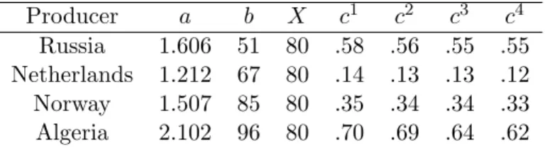
where ai, bi and Xi are parameters. The parameter Xi provides an upper bound on the yearly production of produceri. Values for the parameters indexed by playeriare given in Table 2.1 and values for the parameters indexed by market j are given in Table 2.2.
Table 2.1: Producer parameter values
Producer a b X c1 c2 c3 c4 Russia 1.606 51 80 .58 .56 .55 .55 Netherlands 1.212 67 80 .14 .13 .13 .12 Norway 1.507 85 80 .35 .34 .34 .33 Algeria 2.102 96 80 .70 .69 .64 .62
Table 2.2: Values for price elasticityeand demandD
Market Period 1 Period 2 Period 3 Period 4 BelLux -1.07 0.00 -1.26 0.00 -1.34 0.00 -1.42 0.00
FRGer -1.46 13.70 -1.58 13.80 -1.68 13.80 -1.79 13.80 France -.81 4.80 -1.19 2.90 -1.57 3.00 -2.01 3.00
Italy -1.15 10.40 -1.36 10.00 -1.45 10.00 -1.54 10.40 Netherlands -.94 22.93 -1.13 20.96 -1.29 24.11 -1.45 23.90 UK -.61 33.70 -.87 35.00 -1.10 37.00 -1.30 38.00
The uncertainty in the problem is associated with the price of natural gas in the different markets. The price of natural gas in marketj for time periodt is determined by the total amount of natural gas available annually, as well asξtthe random price of oil in time period t, and is given by
Pt
j(x, ξt) =ptj(ξt) Qt
j(x) qt
In the above equation,Qt
j(x) =Dtj+ P6
i=1xti,j is the total amount of natural gas available in marketjannually throughout time period t. The functionspt
j(ξt) andqjt(ξt) provide the base price and the base demand for natural gas as a function of the price of oil, and are defined as
ptj(ξt) =p0tj ξt/ort
and qjt(ξt) =q0tj ξt/ortηt
with parameters: p0t
j: reference price of natural gas in marketj in time periodt, q0t
j: reference demand for natural gas in marketj in time period t, ort: reference price for oil in time periodt,
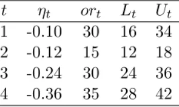
ηt: the elasticity relating the relative demand for natural gas to the relative price of oil. We assume that the prices of oil in each time period are independent and uniformly distributed with lower and upper bounds Lt and Ut. The values for the parameters in the base price and demand functions are given in Tables 2.3 and 2.4.
Table 2.3: Reference prices p0 and demandsq0
Market Period 1 Period 2 Period 3 Period 4 BelLux 5.12 7.8 2.56 9.4 3.41 9.4 5.12 9.5 FRGer 5.27 40.7 2.64 46.2 3.52 46.5 5.27 44.6 France 5.25 23.6 2.62 28.3 3.50 9.8 5.25 28.5 Italy 5.15 25.3 2.57 34.9 3.43 37.5 5.15 37.2 Netherlands 5.16 28.9 2.58 29.9 3.44 32.2 5.16 29.7 UK 4.54 43.8 2.27 50.3 3.03 56.4 4.54 53.7
Table 2.4: Time period parameters in base price demand function
t ηt ort Lt Ut 1 -0.10 30 16 34 2 -0.12 15 12 18 3 -0.24 30 24 36 4 -0.36 35 28 42
each time period we use the factorft to express the future value of money with
ft=
(1 +r)yt−1
r
1 (1 +r)Pts=1ys
! .
The net present value profit function for producer iis then defined to be
Υi(x, ξ) = 4 X t=1 ft 6 X j=1
Pjt(x, ξt)−cti
xti,j−Gi(x)
. (2.13)
Taking the expectation of (2.13) reduces to calculating EhPt j(x, ξt)
i
and provides us with an expression for φi0. Under the assumption that the oil prices are uniformly distributed
we have
E Pt
j(x, ξt)
=p0t
j Qtj(x)q0tj 1/etj
orηt/e
t j−1
t
U2−ηt/e
t j
t −L
2−ηt/etj
t
1
(Ut−Lt)(2−ηt/et j)
.
With expressions for Υi and φi0 we are able to obtain explicit formulas for both f0(x) and
fN(x).
To find solutions to both the true SVI (2.11) and its SAA (2.12) we make use of the fact that S=R96
+. For anyx∈S, the normal cone to S atxis
NS(x) =
v ∈R96|vi = 0 ifxi>0 andvi ≤0 if xi = 0 .
Therefore, the variational inequalities (2.11) and (2.12) are equivalent to the mixed com-plementarity problems (MCPs)
0≤x⊥f0(x)≥0 and 0≤x⊥fN(x)≥0
re-quires evaluating fN(x, ξ), dfN(x, ξ), and the B-derivative of the projection onto S = R96+ at a pointz which is equal to
dΠS(z)(h) =
λ1 · · · 0 ..
. . .. ... 0 · · · λ96
h1 .. . h96
whereλi=
1 (z)i>0,
1 (z)i= 0 and hi≥0, 0 (z)i= 0 and hi≤0, 0 (z)i<0.
The calculation of confidence regions and simultaneous confidence intervals is done in (MAT-LAB, 2010) using the MATLAB/GAMS interface (Ferris, 2005) to pass the SAA and true solutions between programs.
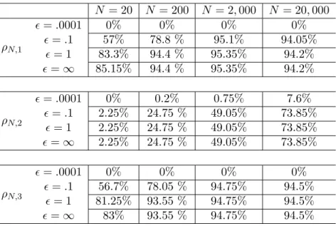
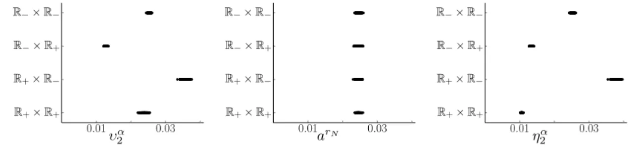
To analyze the performance of the confidence regions and corresponding simultaneous confidence intervals, we generate 2,000 replications of the SAA problem at each sample size ofN =20, 200, 2,000, and 20,000. For each sample,dfN,Snor(zN) is linear and the simultaneous confidence intervals take the form of (2.3). To determine lN, all eigenvalues of ΣN larger than a threshold ρN are treated as nonzero. Three different procedures are considered for choosing the threshold ρN. In the first, ρN,1 = N−1/3, while in the second and third ρN is held constant at ρN,2 = 10−10 and ρN,3 = 0.001 respectively. Note that the choice of ρN,1 will be asymptotically correct if ΣN converges to Σ0 in probability at an exponential rate. This would occur if in Theorem 2 we replace Assumption 1 with Assumption 4. The use of ρN,1 results in four eigenvalues being treated as nonzero across all samples, while the constant thresholds results in values of lN that vary slightly between samples. When ρN,2 is used lN equals either eight or nine and whenρN,3 is used lN equals either four or five. In Table 2.5, we summarize the coverage rates ofz0 by the confidence regionsRN, for each choice of ρN and values of =0.0001, 0.1, 1, and ∞. For example, with the choices of ρN,1 and = 0.1, the true value of z0 is covered by 83.3% of the 95% confidence regions computed from the 2,000 replications atN = 20.
Table 2.5: Coverage rates of confidence regions forz0, α=.05
N = 20 N = 200 N = 2,000 N = 20,000
ρN,1
=.0001 0% 0% 0% 0%
=.1 57% 78.8 % 95.1% 94.05%
= 1 83.3% 94.4 % 95.35% 94.2%
=∞ 85.15% 94.4 % 95.35% 94.2%
ρN,2
=.0001 0% 0.2% 0.75% 7.6% =.1 2.25% 24.75 % 49.05% 73.85%
= 1 2.25% 24.75 % 49.05% 73.85% =∞ 2.25% 24.75 % 49.05% 73.85%
ρN,3
=.0001 0% 0% 0% 0%
=.1 56.7% 78.05 % 94.75% 94.5% = 1 81.25% 93.55 % 94.75% 94.5%
=∞ 83% 93.55 % 94.75% 94.5%
choice oflN is seen in the different coverage rates ofz0 for values of≥0.1. In the liberal classification scheme that uses ρN,2, near zero eigenvalues are included in DN. WhenDN is inverted the reciprocals of these near zero eigenvalues offset the increase in the degrees of freedom of the χ2 random variable on the right hand side of (2.5), resulting in poor coverage of z0. The classification schemes that use ρN,1 and ρN,3 have a higher threshold for treating eigenvalues as nonzero. As a result these thresholds avoid the inclusion of overly large values inDN−1 and produce regions that perform largely in line with the specified level of confidence. The choice of =∞ corresponds to the percentage of samples that satisfy (2.5) and provides an upper bound on the coverage rates.
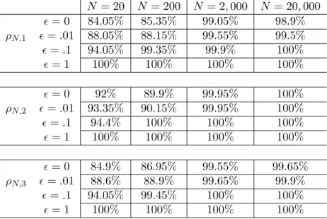
Next, as we examine the performance of simultaneous confidence intervals we observe that their coverage rates keep increasing as increases, and eventually reach 100% for sufficiently large, see Table 2.6. This is consistent with the analytical results in Proposition 1, since for this example each sample and choice or ρN results in w
Table 2.6: Coverage rates of simultaneous confidence intervals forz0,α=.05
N = 20 N = 200 N = 2,000 N = 20,000
ρN,1
= 0 84.05% 85.35% 99.05% 98.9% =.01 88.05% 88.15% 99.55% 99.5%
=.1 94.05% 99.35% 99.9% 100%
= 1 100% 100% 100% 100%
ρN,2
= 0 92% 89.9% 99.95% 100%
=.01 93.35% 90.15% 99.95% 100%
=.1 94.4% 100% 100% 100%
= 1 100% 100% 100% 100%
ρN,3
= 0 84.9% 86.95% 99.55% 99.65%
=.01 88.6% 88.9% 99.65% 99.9%
=.1 94.05% 99.45% 100% 100%
= 1 100% 100% 100% 100%
but for the larger sample sizes do so at a conservative rate. The conservative performance at small values of is most obvious with the choice of ρN,2. As noted after Proposition 1 treating more eigenvalues as nonzero increases the intercept term of (2.7), which increases the interval’s length forsufficiently small.
Next, we examine the computation of individual confidence intervals, and compare them with the simultaneous confidence intervals. In this example df0nor,S(z0) is linear and df0nor,S(z0)−1Σ0df0nor,S(z0)−T has nonzero diagonal elements. Therefore, by Theorem 3, the formula (1.21) will provide asymptotically exact intervals for this example. Using this for-mula we consider individual confidence intervals at both α = .05 and with a Bonferroni adjustment ofα0 = .9605. Below, we refer to intervals produced using the Bonferroni adjust-ment as adjusted confidence intervals, and will examine their performance as simultaneous confidence intervals.
inter-vals are 88.2%, 88.4%, 99.75%, and 99.75%, respectively. These rates are comparable to the coverage rates of the simultaneous confidence intervals calculated using (2.4) for small values ofas given in Table 2.6.
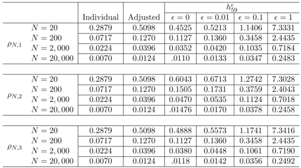
To observe differences between the adjusted and simultaneous confidence intervals we compare their interval lengths. Table 2.7 summarizes the half widths of the individual, adjusted, and simultaneous confidence intervals for (z0)59 for a single replication at each sample size. Half widths of the individual and adjusted confidence intervals do not depend onρN. However, in Table 2.7 their values are repeated for each choice ofρN, to be compared with the corresponding simultaneous confidence intervals. With the choice ofρN,2, even the
Table 2.7: Half-widths of intervals for (z0)59,α=.05
h 59
Individual Adjusted = 0 = 0.01 = 0.1 = 1
ρN,1
N = 20 0.2879 0.5098 0.4525 0.5213 1.1406 7.3331 N = 200 0.0717 0.1270 0.1127 0.1360 0.3458 2.4435 N = 2,000 0.0224 0.0396 0.0352 0.0420 0.1035 0.7184 N = 20,000 0.0070 0.0124 .0110 0.0133 0.0347 0.2483
ρN,2
N = 20 0.2879 0.5098 0.6043 0.6713 1.2742 7.3028 N = 200 0.0717 0.1270 0.1505 0.1731 0.3759 2.4043 N = 2,000 0.0224 0.0396 0.0470 0.0535 0.1124 0.7018 N = 20,000 0.0070 0.0124 .01476 0.0170 0.0378 0.2458
ρN,3
N = 20 0.2879 0.5098 0.4888 0.5573 1.1741 7.3416 N = 200 0.0717 0.1270 0.1127 0.1360 0.3458 2.4435 N = 2,000 0.0224 0.0396 0.0380 0.0448 0.1061 0.7190 N = 20,000 0.0070 0.0124 .0118 0.0142 0.0356 0.2492
used, this value ofis between 8.86×10⁻⁴ and 0.1728, and between 3.57×10⁻⁴ and 0.1395 when using ρN,3.
As noted after Proposition 1, the choice of lN determines the degrees of freedom of the χ2 random variable, as well as the upper index of summation in the intercept, and the lower index of summation in the slope of w
N,j. When comparing interval lengths for different choices of ρN and = 0, the differences are largely the result of changes in the degrees of freedom of the χ2 random variable. This is seen by comparing the ratio of w0
N,j
for two choices of ρN to the ratio of the square root of χ2lN for the same choices of ρN.
The difference between these two ratios is on the order of 10−4 across all components and samples.
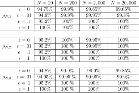
So far, we have considered only confidence regions and intervals forz0, the true solution to the normal map formulation. In most problems, the true solution to the variational inequality, namely x0, has a more direct interpretation and is of greater interest. The relation ΠS(z0) =x0 and the easily observed fact that
Pr (z0 ∈IN(ω))≤Pr (ΠS(z0)∈ΠS(IN(ω))), for any random setIN(ω),
provides one indirect approach for obtaining confidence intervals for x0 that cover the true solution with a rate that is at least as large as the coverage rate of z0 by IN(ω). With S =R96
+, projecting the simultaneous confidence intervals forz0ontoS reduces to replacing negative endpoints of these intervals with zero. Comparing the coverage rates of x0, as summarized in Table 2.8, to the coverage rates ofz0, we observe the largest increase for the smaller sample sizes and values of .
The expression forw
N,j in (2.7) and the analysis of this example provides useful insights for choosing and lN when the sample covariance matrix is singular. When choosing lN care should be taken to avoid classifying overly small eigenvalues as nonzero. In the case of confidence regions, such care can prevent poor coverage performance due to large elements of D−1
Table 2.8: Coverage rates of simultaneous confidence intervals forx0,α=.05
N = 20 N = 200 N = 2,000 N = 20,000
ρN,1
= 0 94.75% 99.9% 99.65% 99.65%
=.01 94.9% 99.9% 99.95% 99.8%
=.1 95.2% 100% 100% 100%
= 1 100% 100% 100% 100%
ρN,2
= 0 95.2% 100% 99.95% 100%
=.01 95.2% 100 % 99.95% 100%
=.1 95.2% 100 % 100% 100%
= 1 100% 100 % 100% 100%
ρN,3
= 0 94.8% 99.9% 99.9% 99.85%
=.01 94.95% 99.95 % 99.95% 99.9%
=.1 95.2% 100 % 100% 100%
= 1 100% 100 % 100% 100%
When the confidence regions are the primary set of interest, small values of often lead to poor coverage performance, and there is an upper bound on the coverage rate asgoes to infinity. These properties suggest choosing a larger value of to obtain the desired level of coverage by the confidence regions. When the confidence regions are to be used to build simultaneous confidence intervals for z0 or x0, a small value of , even the extreme choice of= 0, appears appropriate. This is based on the expression forw
CHAPTER 3
Confidence intervals for the normal map solution
3.1 Introduction
This chapter presents two new methods for constructing individual confidence intervals for the normal map formulation of an SVI. For both methods, a level of confidence can be specified under general situations. While our main interest is on SVIs and their normal map formulations, the ideas of those two methods work for general piecewise linear functions. We outline the ideas below, and leave formal definitions and proofs to§3.2 and§3.3. Recalling the notation introduced in Chapter 1, we use (v)j to denote the jth coordinate of a vector v, and (M)j to denote the jth row of a matrix M. Similarly for an invertible function f : Rn→Rn, (f)j will denote thejth component function of f and (f−1)j thejth component function of f−1.
Suppose f :Rn → Rn is a piecewise linear homeomorphism with a family of selection functions {M1, . . . , Ml} and the corresponding conical subdivision {K1, . . . , Kl}, so f is represented by the linear map Mi when restricted to Ki. SupposezN is an n-dimensional random vector such that√N(zN−z0)⇒f−1(Z), wherez0∈Rnis an unknown parameter, Z ∼ N(0, In), and In is the n×nidentity matrix. Our objective is to obtain a confidence interval for (z0)j, j = 1,· · ·, n. The idea of the first method is to look for a number a such that Pr(|(f−1)j(Z)| ≤a) equals a prescribed confidence level, and then use [(zN)j− aN−1/2,(zN)j+aN−1/2] as the interval. For situations considered in this chapter, z