a quantum random access memory
THESIS
submitted in partial fulfillment of the requirements for the degree of
MASTER OFSCIENCE in
PHYSICS
Author : Arnau Sala Cadellans
Student ID : S-1441426
Supervisor : C. W. J. Beenakker
2nd corrector : Miriam Blaauboer
a quantum random access memory
Arnau Sala Cadellans
Instituut-Lorentz, Leiden University, P.O. Box 9500, 2300 RA Leiden, The Netherlands
Kavli Institute of Nanoscience, Delft University of Technology, Lorentzweg 1, 2628 CJ Delft, The Netherlands
June 29, 2015
Abstract
In this thesis, the necessary elements to build up a quantum switch, the central element in a quantum random access memory, are proposed and
analyzed. A network with quantum switches at its nodes forms the bifurcation path that leads an address register from a root node to an array of memory cells, activating, quantum coherently, only the quantum
switches that the register encounters in its path to the memory cells. Transmon qubits and SQUIDs are used to design a superconducting device capable of routing a register of microwave photons through a bifurcation network, allowing for superposition of paths. In order to give
rise to all the required interactions between the device and the address register, a non-linear capacitor, composed of two plates with carbon nanotubes in between, is introduced into the transmon. The dynamic operation of the quantum switch is analyzed using Langevin equations
and a scattering approach, and probabilities of reflection and transmission of photons by (or through) the switch are computed, both
for single- and two-photon processes. Computations show that, with parameters taken from up-to-date similar devices, probabilities of
success are above 94%. Applications of quantum random access memories are discussed, as well as other applications of quantum switches. Also, solutions are proposed to the challenges that emerge
1 Introduction 1
1.1 Quantum information processing 1
1.2 Why a quantum RAM? Quantum memory theory 2
1.2.1 Quantum memory implementation 4
1.3 Other attempts 4
1.4 Thesis outline 5
2 The Quantum Switch as a central element 7
2.1 A first guess 7
2.2 The need for a non-linear element 10
2.3 A multilevel device using non-linear capacitors 12
2.4 Frequency filters in the transmission lines 17
2.5 An alternative solution 19
3 Analysis of the model and further considerations 29
3.1 Quantizing the Hamiltonian 29
3.2 Dynamics of operation and a problem with the transmon 36
3.2.1 Operation 37
3.2.2 Scalability 39
3.3 The final Hamiltonian 40
3.4 Relaxation and dephasing 43
3.5 Equations of motion 46
4 Dynamics of operation of the Quantum Switch 51
4.1 Scattering of a single photon 51
4.1.1 Probability 55
4.2 Two-photon processes 55
4.3.1 Without decoherence 62
4.3.2 With decoherence 71
5 Implementation of the Quantum Switch into a QRAM 75
5.1 Not all the requirements can be fulfilled 75
5.2 How to get to the memory cells 77
5.3 Retrieval of information 79
6 The Switch beyond the QRAM 83
6.1 The switch as a single element 83
6.1.1 Creation of entanglement 84
6.1.2 Amplification of single-photon signals 85
6.1.3 Measurement of the frequency of a single photon 85
7 Conclusions 87
Appendices 89
A Lagrangians and Hamiltonians in cQED 91
A.1 Quantization of the Hamiltonian 93
A.2 Transmission lines 95
B Coefficients in the Hamiltonians 97
B.1 Hamiltonian in Section 2.3 97
B.2 Hamiltonian in the Section 2.5 101
C Equations of motion within thein/outformalism 105
D Derivation of single-photon scattering amplitudes 109
E Failed attempts (1): numerical integration 117
E.1 Schr¨odinger picture 118
E.2 Heisenberg picture 119
F Failed attempts (2): propagators and Green’s functions 123
G Failed attempts (3): Feynman diagrams 127
G.1 Propagators within the free field theory 128
G.2 Fromn-point correlation functions to theS-matrix 130
G.3 Feynman rules 131
Chapter
1
Introduction
1.1
Quantum information processing
It is even possible to combine these disciplines to create a hybrid device [10]. Though in all these cases only few qubits were considered, there is no reason to believe that a larger device, capable of handling more inputs, cannot be con-structed [4,7,13].
In any case, to perform quantum computations, a universal quantum computer must be capable of storing information within quantum states to use it later in a further stage of an algorithm and it must also have access to classical (or quantum) data as a superposition of the entries. Examples of algorithms with these require-ment are the Grover search [11] and the Deutsch-Jozsa [11] algorithms. For these reasons, just like a classical computer needs a processor capable of doing classical operations and a memory to keep and extract the data, a quantum computer also needs some sort of RAM memory able to handle quantum information.
1.2
Why a quantum RAM? Quantum memory
the-ory
Any computer needs some memory device for storing or extracting information. Given that current computers work with may bits, this device has to be composed of multiple instances of “memory cells” where single bits can be stored. Nowa-days, the device used for these purposes is a random access memory (RAM), which is a device whose memory cells can be addressed at will (randomly) in-stead of sequentially (like in a CD or a hard drive). This instrument [14] consists of an array of memory cells, where the information (bits) is kept, and an electronic circuit in a tree-like structure that routes an “address register” from a root node –connected to the processor– to each of the memory cells, as shown in FIG.1.1. When the address register –which contains the instructions to reach the desired memory cell– is sent to the memory device, a path through the tree-like circuit that leads to the target cell is opened. Common RAM memories composed of N=2n memory cells require the manipulation ofN−1 nodes of the bifurcation path.
Memory cells
Root node 0
1 2 3 4
0 1 2 3 4 5 6 7 8 9 10 11 12 13 14 15 16 17 18 19 20 21 22 23 24 25 26 27 28 29 30 31
Figure 1.1: A common random access memory can be schematically represented with this diagram [14]. This diagram contains a root node in the 0th level that bifurcates into two transmission lines (solid gray). A switch at every node (black) decides which path leads to the chosen memory cell and which paths remain unconnected.
An interesting architecture (the bucket brigade architecture) for a quantum random access memory (QRAM) was proposed by Giovannetti, Lloyd and Mac-cone [15]. It consists of a device similar to FIG.1.1but with quantum switches at the nodes. These quantum switches are elements that can be in three states, one of them being a ground state and the other two being excited states. The ground state is thewaitstate: the path is closed. The other two excited states are either leftorright(open the path that goes to the left/right). Given the quantum nature of the switch, it is also possible to prepare it in the stateleft and right.
Within this scheme, to evaluate a memory cell, an initial register is needed. This register contains the instructions to reach the target cell: if the path from the root node to the cell is root-left-left-right-left-right, then the first element of the register containsleft, the second containsleft, etc. One more element in the regis-ter is needed to inregis-teract with the content of the memory cells and bring back the information it stores. When the register reaches the root node, the quantum switch reads (and keeps) its first element and evolves fromwaittoleft. The register con-tinues (without its first element) to the second node and so on. After the register has gone through all the nodes, a single element is left. This element reads the content of the memory cell and is emitted back through the path that is still open. If instead of a classically-defined register a quantum register with a superposition of states is sent in, the output would be a superposition of the content of the mem-ory cells evaluated.
manip-ulation and entanglement of O(N) quantum switches whereas, with the bucket brigade architecture onlyO(log(N))switches must be thrown, thus reducing the number of elements that have to be coherently entangled.
The benefits of working with a QRAM include the possibility of realizing algorithms that require the manipulation of data in a superposition state and the possibility of sending a query and receiving an answer with total anonymity: if instead of a definite question (evaluation of a memory cell) a superposition of questions is sent, an output with a superposition of answers will be sent back, and only who has a complete knowledge of the original question can extract the right answer out of the output [16].
1.2.1
Quantum memory implementation
The most important element of a QRAM, that makes it different from any other device capable of storing information, is the quantum switch that routes the in-coming register through the right path to the memory array. This element can in principle be realized with many different elements, but only a solid-state imple-mentation, using superconducting qubits, will be discussed. This choice has been made based on the simplicity of its structure –it is analytically tractable and easy to fabricate– and the apparently small probability of errors, as various authors show in their single-photon transistors based on circuit quantum electrodynamics (cQED) [17, 18] or nanoscale surface plasmons [19]. A superconducting-based device can be combined with other systems, such as diamonds [10], etc.
The other basic element of a memory, the array of memory cells, can be re-alized in multiple ways –it can be a quantum device or a classical memory with only classical information– without affecting the dynamics of operation described previously and it is not in the focus of this project.
Thus, the device to be developed must absorb the first element of a register composed of photons –microwave photons, since these are the kinetic elements in cQED systems– and route the rest of the photons, independently of their state, according of the state of the absorbed photon.
1.3
Other attempts
gate implementation, using phase shifters (e.g. superconducting qubits) and mi-crowave photons is discussed in the same paper [20]. Alternatively, the authors propose to use multilevel atoms controlled by lasers to induce Raman transitions so they absorb and emit photonic registers. Other alternatives have been proposed, such as using a beam splitter based on Superconducting Quantum Interference De-vices (SQUID) to route some photons carrying the information through the desired path [21]. Others propose to use toroidal resonators as quantum switches [22].
Regarding the beam splitters (BS), there has been some research too. In ref-erences [23–25] the authors use cQED devices to act as BS in a way such that there are two incoming photons through two different transmission lines and the BS sends the input photons to one of the outgoing transmission lines, or both, creating an entangled state or just separating even modes from odd modes. This option is in disagreement with the structure of a QRAM (or a RAM) because there is a single incoming transmission line that bifurcates several times, whereas the authors consider multiple incoming transmission lines. The authors in [26] have designed a beam splitter that separates an incoming photon into even and odd modes. This design is not useful either because once the modes have been sep-arated the beam cannot be split again, thus it is not possible to create a tree-like structure with more than one node. Finally, other authors [27] have designed a device that can send a photon to one transmission line or another depending on its frequency. With this device, a photon that goes to the left in one node will go to the left in all the successive nodes as well, so it may not be a good option because the only two memory cells accessible from the root node would be the rightmost node and the leftmost node.
1.4
Thesis outline
During this project I have proposed and analyzed the necessary elements to build up a quantum random access memory with the architecture proposed by Giovan-netti et al. in [15]. Transmon qubits and SQUIDs are used to design a multi-level system, mimicking artificial atoms with non-linear energy multi-levels, capable of routing a register from the root node to the target cell minimizing the quantum decoherence processes. The register is sent via microwave photons through su-perconducting waveguides (transmission lines).
conducted to check that no more elements are needed and that the switch can, in principle, work as expected. A Lagrangian of the system is derived in this section. In the third chapter, an in-depth analysis of the device is conducted. A Hamil-tonian, derived from the Lagrangian, is quantized and the equations of motion, containing relaxation and dephasing elements, are obtained. The fourth chapter contains the calculation of scattering amplitudes and probabilities of reflection and transmission processes involving one and two photons. Numerical calculations, with realistic parameters, are carried out to check the performance of the quantum switch. The dynamics of operation of this device is derived in this chapter. The possibility of implementing this element into a quantum random access memory is treated in the chapter 5. The sixth chapter contains an interesting discussion of the possibilities of the quantum switch beyond a QRAM.
Chapter
2
The Quantum Switch as a central
element
2.1
A first guess
In order to find the right elements that compose a quantum switch it is convenient to write down a basic Hamiltonian containing all the necessary terms to gener-ate the desired interaction. Once the Hamiltonian has been set, we can proceed to find the physical elements –capacitors, inductors, Josephson junctions or other elements of cQED systems– corresponding to each term of the Hamiltonian. To make this process simpler, let us first consider the case where only one incoming transmission line and only one outgoing transmission line are present. This sim-plified quantum switch has to decide whether the incoming photons (the address register) can be transmitted or not.
As explained before, the address register consists of an array of photons. Each of the photons can be in two states (or a superposition) that tells the quantum switch in which directions the other photons of the register have to be forwarded. These states are defined by the energy of the photons.
kinetic terms describing the energy of the levels ofT andS
H0=ωT1a†T1aT1+ωT2a†T2aT2+ωS1a†S1aS1+ωS2a†S2aS2. (2.1)
In this equation,a†T1 anda†T2 are the ladder operators that excite the levels ofT. a†S1anda†S2 are the ladder operators that excite the levels ofS. Since the photons can only be in two states, with energiesωT1andωT2, I have only considered the
two lowest energy levels ofT andS. The energies of the levels satisfyωT1<ωT2
andωS1<ωS2. I have also chosen ωT2−ωT16=ωT1 to make sure that it is not
possible to excite the second level ofT (ωT2) by sending two photons with energy
ωT1each. If that were the case, the control element would absorb also the second
photon of the register instead of forwarding it. Moreover, there has to be an extra term that, in case that the levels ofT are occupied, enforces a shift in the energies ofS, so they can be excited by incoming photons with energiesωT1andωT2.
HJ=−J11a†T1aT1a†S1aS1−J12a†T1aT1a†S2aS2
−J21a†T2aT2a†S1aS1−J22a†T2aT2a†S2aS2. (2.2)
The elements withJi jdecrease the energy of the j-th level in theSatom when the
i-th level in theT atom is occupied. I have also included a term that couples T andS to the transmission lines. Actually this term has to couple T andS to the incoming transmission line and onlySto the outgoing transmission line, because the photon absorbed byT must not be transmitted.
Hc= a
† T1bω √
π τ +
a†T2bω
√
π τ +
a†S1bω
√
π τ +
a†S2bω
√
π τ +
a†S1cω
√
π τ +
a†S2cω
√
π τ +
h.c. (2.3)
Herebandcare the frequency-dependent ladder operators for the incoming and outgoing transmission lines, respectively. A momentum integral should be in-cluded in this expression to account for all the possible momenta an incoming (or outgoing) photon can have. The coupling constant, which in this simple case I make the same for all the possible processes, has this form to show its explicit dependence on the lifetimeτ of the atomic excitations. This equation shows how
a photon (borc) is absorbed (and emitted) by theT orSatom-like elements.
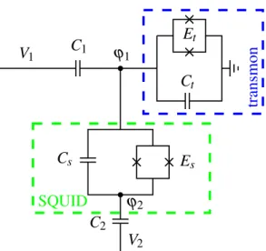
V1 C1 ϕ1
Et
Ct
Cs Es
ϕ2
C2 V2
SQUID
transmon
Figure 2.1: A candidate for a device whose Hamiltonian contains all the desired inter-actions could be this system composed of a transmon qubit (blue box) with Josephson energy Et and a SQUID (green box) with Josephson energy Es. They are capacitively
coupled to an incoming transmission line with potentialV1and an outgoing transmission line with potentialV2. At each node of the circuit a flux can be defined. These are the dynamical variables of the system.
L=C1
2 (ϕ˙1−V1)
2+C2
2 (ϕ˙2−V2)
2+Cs
2 (ϕ˙1−ϕ˙2)
2+Ct
2ϕ˙
2 1
+Etcos
ϕ1
ϕ0
+Escos
ϕ1−ϕ2
ϕ0
, (2.4)
H= 1
2γ
p21+C1+Cs+Ct
C2+Cs
p22+ 2Cs
C2+Cs
p1p2
+2C1V1p1+2
C2Cs
C2+Cs
V2p1
+2C2
C1+Cs+Ct
C2+Cs V2p2+2 C1Cs
C2+CsV1p2
−Etcos
ϕ1
ϕ0
−Escos
ϕ1−ϕ2
ϕ0
, (2.5)
whereϕ0=h¯/2eis the flux quantum divided by 2π, p1and p2are the
conju-gate momenta ofϕ1 andϕ2andγ =C1+Ct+CsCsC+C22. This Hamiltonian contains
the capacitances it is possible to weaken the interaction between the transmon and the outgoing transmission line (V2), so the photons absorbed by the transmon are
never transmitted forward. From the cosines it is possible obtainHJ after expand-ing them in a Taylor series and quantizexpand-ing the fluxes∗.
Let me now analyze with more detail the Eq. (2.1, 2.2, 2.3). a†T1 excites the first level of a multilevel system, whereasa†T2excites a second –or higher– level. These are given by a ladder operator and some power of ladder operators, re-spectively. This means that, before quantizing the Hamiltonian, there should be different powers of the momenta or the fluxesϕ1andϕ2–such as p41orϕ14; these
may come from the cosines– and also powers of the fluxes times the potential, such as p31V1†, that describe how the highest energy level of the transmon (or the SQUID) is excited directly from the ground state with a single photon. These last elements are not in the Hamiltonian derived from (2.4).
2.2
The need for a non-linear element
A Hamiltonian that describes a transmission line coupled to the third level of a transmon –a transmon whose higher energy levels can be excited by the absorp-tion of a single photon, without the need to go through all the lower levels– must contain either p31V1 or ϕ13V1. Alternatively, it can contain a function with e.g.
p1+V1 in its argument such that its Taylor expansion gives rise to the desired
interaction.
In cQED circuits there are typically two kinds of elements: capacitive ele-ments, whose energy depends on the derivative of fluxes and on potentials; and inductive elements, whose energy depends only on the fluxes, such as inductors or Josephson junctions [29]. An inductive element cannot depend onϕ−V‡, the
element to be introduced in the system has to be a capacitive element. If this is a capacitor whose capacitance is a non-linear function of the potential –and its energy is not a quadratic function of the potential–, the Hamiltonian may contain a function that depends on ˙ϕ andV and whose Taylor expansion will give rise to
the desired terms§. ∗See AppendixA
†The Hamiltonian must contain even powers of operators to ensure that the energy is
con-served (bounded from below). Thus, the coupling to the transmission lines is given byp31V1. This
means that the third –and not the second– level of the transmon (or the SQUID) is coupled to the transmission lines. This coupling is obtained in Chapter3.
‡This follows from the Kirchhoff’s circuit laws and the dependence of the current on the flux
and momentum for the different inductive elements [30].
Non-linear capacitors are not common in this kind of circuits, but they have been studied for decades. In the related literature capacitors with two different non-linear behaviors can be found. Some of them are made of ferroelectric thin films or ferroelectric ceramics and show a capacitance that decreases with the applied voltage [31–33]. Others show a capacitance that increase with the volt-age, such as those made out of antiferroelectric materials [34] or semiconductor devices that, under some conditions, behave as non-linear capacitors due to the presence of a space charge near a junction [35].
There is another well studied semiconductor device that show both behaviors: the MOS capacitor. Depending on whether it is a p-type or a n-type MOS, it will exhibit a capacitance that increases or decreases with the voltage [36–38].
Some work has been done on the quantum level as well. The capacitance due to the presence of quantum wells in heterojunctions gives rise to a strong non-linear behavior of the capacitor, whose capacitance drops off very fast with small variations of the potential [39]. Another source of non-linear behavior is the finite-ness of the density of states (DOS) in small devices. For a two-plate capacitor, this gives rise to a capacitance that decreases for increasing potential [40]. But, if car-bon nanotubes are placed between the plates of the capacitor, due to the finiteness of the DOS of the nanotubes the capacitance will increase with small variations of the potential [41,42].
In the model I propose I am using a non-linear capacitor with a behavior sim-ilar to the last one. For simplicity I have used a curve forC(V)(capacitance as a function of the potential across the plates of the capacitor) only valid nearV →0, given that only (small) quantum fluctuations ofV have been considered. The ca-pacitance as a function of the potential I have used is
C(V) =C0+C1V2. (2.6)
does not contain terms such asa† ora†a†a(odd powers of the momentum or the flux) is to use Eq. (4.33) for the voltage dependence of the capacitor, leading to an energy function of the form
E(V) =C
2 V
2+
αV4. (2.7)
As will be shown later on (Section2.5), the odd energy levels of a transmon constructed with this capacitor are coupled to the transmission lines, whereas the even levels are not. It is only possible to excite an even level if an odd (inferior) level had been excited first.
2.3
A multilevel device using non-linear capacitors
Consider the system shown in FIG.2.2. It contains the three required transmission lines. This device is composed of a transmon qubit with a non-linear capacitor and two SQUIDs with linear capacitors. I have not included non-linear capacitors on the SQUIDs because they would make impossible to perform the Legendre trans-formation of the Lagrangian analytically. Moreover, with one non-linear capacitor is enough to generate all the desired interactions. Using Eq. (2.7) for the energy of the nonlinear capacitor in the transmon, the Lagrangian of this system reads
L=C1
2 (ϕ˙1−V1)
2
+C2
2 (ϕ˙2−V2)
2
+C3
2 (ϕ˙3−V3)
2
+Cs2
2 (ϕ˙1−ϕ˙2)
2+Cs3
2 (ϕ˙1−ϕ˙3)
2+Ct
2 ϕ˙
2
1+αtϕ˙14
+EJtcos
ϕ1
ϕ0
+EJ2cos
ϕ1−ϕ2
ϕ0
+EJ3cos
ϕ1−ϕ3
ϕ0
. (2.8)
Despite the presence of the nonlinear equation, the Hamiltonian can be con-structed analytically with the conjugate momenta p1, p2 and p3 and the fluxes defined, as a function of the momenta, as
˙
ϕ1=
21/3γ
f(x) −
f(x)
21/3β (2.9)
˙
ϕ2=
p2+C2V2+Cs2ϕ˙1
C2+Cs2 (2.10)
˙
ϕ3=
p3+C3V3+Cs3ϕ˙1
C3+Cs3
V1
V3
V2 C2
Cs2 Cs3
EJ2
EJt
EJ3 C3
Ct
ϕ3
ϕ1
ϕ2
C1
Figure 2.2: This system contains one incoming (V1) and two outgoing (V2,V3) transmis-sion lines. It is composed of a transmon with a non-linear capacitor (Ct) and two SQUIDs
with linear capacitors (the symbol used for the non-linear capacitor is also a commonly used symbol for capacitors, especially in the US, but is not the generic).
with
f(x) =
−3β2x+
q
4β3γ3+ (3β2x)2
1/3
(2.12)
β =6Ctαt (2.13)
γ=C1+Ct+
C2Cs2
C2+Cs2
+ C3Cs3
C3+Cs3
(2.14)
x=p1+C1V1+ Cs2
C2+Cs2(p2+C2V2) + Cs3
in the equation, i.e., a product of up to twelve momenta (each of them contains one ladder operator, and a total of 12 is needed). To obtain this term, the Taylor expansion of the Hamiltonian goes up to the twelfth order:
H=p
2
2+2p2C2V2−Cs2C2V22
2(C2+Cs2)
+ p
2
3+2p3C3V3−Cs3C3V32
2(C3+Cs3)
−C1V 2 1
2
+ x
2
2γ − βx4
12γ4+ β2x6
18γ7− β3x8
18γ10+
11β4x10
162γ13 −
91β5x12
927γ16
−EJtcos
ϕ1
ϕ0
−EJ2cos
ϕ1−ϕ2
ϕ0
−EJ3cos
ϕ1−ϕ3
ϕ0
. (2.16)
After replacing x by the expression in Eq. (2.15), the Hamiltonian contains V12p21,V13p2, etc, which describe the process where one or several transmon states decay into more than one photon in the transmission lines or several photons are absorbed by the transmon at the same time. These processes must be eliminated. To do so I have expanded the Hamiltonian in a power series ofV1,V2andV3 and
I have checked under what conditions on the capacitances terms of orderO(V2)
can be omitted (C1,Cs2,Cs3smaller thatC2,C3).
Next I have also also expanded the Hamiltonian in Eq. (2.16) for p1, p2 and p3, keeping only the largest terms, up to orderO(p6)–that is, keeping p61and also p61p62. The final equation can be separated in six parts, each of them describing a different behavior. The first equation,H1, contains even powers of the momenta and the fluxes without mixing them. From this expression, the Hamiltonian de-scribing the energy of the levels can be derived.
H1=
1 2γp
2 1+
1
2(C2+Cs2)+
C2s2
2(C2+Cs2)2γ
p22
+
1
2(C3+Cs3)+
Cs23
2(C3+Cs3)2γ
p23
− β
12γ4p
4 1−
Cs42β
12(C2+Cs2)4γ4p 4 2−
Cs43β
12(C3+Cs3)4γ4p 4 3
+ β
2
18γ7p
6 1+
Cs62β2
18(C2+Cs2)6γ7p 6 2+
Cs63β2
18(C3+Cs3)6γ7p 6 3
−(EJt+EJ2+EJ3)cos
ϕ1
ϕ0
−EJ2cos
ϕ2
ϕ0
−EJ3cos
ϕ3
ϕ0
. (2.17)
describes the coupling between the energy levels. It contains products of even powers of the momenta and also the fluxes:
H2= 3
∑
i=1 j>i
3
∑
m=1 3
∑
n=1
Ai jmnp2imp2jn
−EJ2
cos ϕ1 ϕ0
−1 cos
ϕ2 ϕ0 −1
−EJ3
cos ϕ1 ϕ0
−1 cos
ϕ3 ϕ0 −1 . (2.18)
The coefficients Ai jmn can be found in the AppendixB. The interaction with the transmission lines, also obtained by expanding the Hamiltonian in Eq. (2.16), is described by
H3=
C1V1+
Cs2C2V2
Cs2+C2+
Cs3C3V3
Cs3+C3
1
γp1
−
C1V1+
Cs2C2V2
Cs2+C2+
Cs3C3V3
Cs3+C3
β
3γ4
p31
+
C1V1+
Cs2C2V2
Cs2+C2+
Cs3C3V3
Cs3+C3
Cs2
(Cs2+C2)γ
+ C2V2
(Cs2+C2)
p2
−
C1V1+Cs2C2V2
Cs2+C2
+Cs3C3V3
Cs3+C3
β
3γ4
Cs2
Cs2+C2
3
p32
+
C1V1+Cs2C2V2
Cs2+C2
+Cs3C3V3
Cs3+C3
Cs3
(Cs3+C3)γ
+ C3V3
(Cs3+C3)
p3
−
C1V1+Cs2C2V2
Cs2+C2
+Cs3C3V3
Cs3+C3
β
3γ4
Cs3
Cs3+C3
3
p33. (2.19)
This expression shows that only the odd levels of the transmon (and the SQUIDs) are coupled to the transmission lines. For another choice of the capacitance be-havior a different system may be obtained, e.g., a system that couples also the even levels of the transmon with the transmission lines¶.
In the present system, there is also a term (H4) that describes an exchange
interaction between the transmon and the SQUIDsk.
¶But within these Hamiltonians, other terms that do not conserve the energy and the particle
numbers would emerge.
H4=
3
∑
n=1 3
∑
m=1
B2nmp21n−1p22m−1+B3nmp21n−1p23m−1
−EJ2sin
ϕ1
ϕ0
sin
ϕ2
ϕ0
−EJ3sin
ϕ1
ϕ0
sin
ϕ3
ϕ0
. (2.20)
Again, the coefficientsB2nm and B3nm are found in the AppendixB. The
Hamil-tonianH5, displayed in Eq. (B.1), describes processes such as the annihilation of two excitations of the transmon and the creation of an excitation on one SQUID and an outgoing photon in the transmission lines. In such processes, the informa-tion contained in the photons is lost.
Finally, there is another expression that contains SQUID and SQUID-SQUID-transmon exchange interactions. This expression is not included in the thesis due to its extension, but is not a relevant expression because a slightly dif-ferent system will be introduced (in the following sections) that do not present this interactions. In the previous expressions the terms describing only the transmis-sion lines have been omitted. They will be included a posteriori.
Although it contains the terms that are required for a quantum switch, this Hamiltonian presents some problems:
a) One of them is the HamiltonianH4. Within this expression, the sine functions can be tuned to make them cancel some of the terms, but not all of them. There are some undesired interactions left.
b) Another problematic expression isH5. According to this expression, an exci-tation in the SQUID can decay into a lower exciexci-tation of the transmon plus an outgoing photon in the transmission lines. In this case, the outgoing photon would lose the information it contained and the device would not work prop-erly due to the presence of an excitation where it should not be. The interaction strengths of these processes are too large –compared to those ofH3– to neglect
them.
c) Finally, the SQUID-SQUID and SQUID-SQUID-transmon exchange interac-tions also threaten to give important errors. During the process of transmission of a photon it is important to control exactly which levels are excited and which are not.
H1,H2andH3because these describe the correct operation of the quantum switch I am looking for. These solutions could be:
i) Regarding H4, I can get rid of it by introducing some inductive elements between the SQUIDs, such as a pair of Josephson junctions or a coil. The Hamiltonian of these elements contains a cosine of the fluxesϕ2−ϕ3(in the
case of a Josephson junction) whose Taylor expansion will cancelH4.
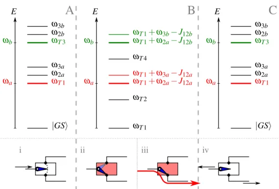
ii) The HamiltonianH5, on the other hand, is more tricky. Imagine that a photon is sent to the switch. This photon can have energies ω1 or ω2. I am only
interested in two processes –considering now that there is only one outgoing transmission line– namely: either the incoming photon with frequency ω1
(ω2) is absorbed and reflected back with energyω1(ω2) or it is absorbed and
transmitted forward with energyω10 (ω20). The expressionH5 describes other
possibilities such as the emission of a photon with energyω100<ω10 with the
subsequent loss of information because it is not possible to know what was the previous state of the photon before the interaction took place and is also not possible to know what interaction took place. To avoid these processes some kind of filters can be introduced in the transmission lines such that they only accept photons that have the right energy. In this way the processes contained inH5cannot happen. Special care has to be taken when introducing these new elements because they may modify the entire Hamiltonian.
2.4
Frequency filters in the transmission lines
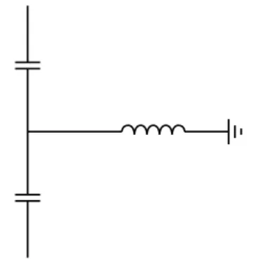
Different kinds of filters can be found in the electronics literature [43]. Some of them contain resistors, other contain capacitors and inductors, etc. Given that the cQED elements used in this work are capacitors and inductors, these are the filters I am considering to use. The high pass LC filter, schematically drawn in FIG.2.3
seems to be the adequate device: it does not allow photons with frequencies below
ω1and photons with higher frequencies pass through.
The Hamiltonian describing the device in FIG.2.3is given by (see [30])
Hhp = 1
2(C1+C2)
p2+ C1V1
C1+C2
p+ C2V2
C1+C2
p
− C1C2
2(C1+C2)(V1+V2)
2+ϕ2
Figure 2.3:Diagram of a high pass LC circuit containing two capacitors and an inductor. At one end of the circuit (e.g., at the top) there is the whole quantum switch and at the other end (bottom) there is one outgoing transmission line.
Once quantized it reads∗∗
Hhp,q=ω1a†a+ Z
d p b
†
1a+a†b1 √
π τ1
+b
†
2a+a†b2 √
π τ2
!
+
Z
d p p
b†1b1+b†2b2
.
(2.22)
According to this Hamiltonian, when a photon (b†) with frequency ω <ω1
(ω1is the threshold frequency) goes in it is reflected, because it cannot excite the
system. If the frequency isω1, then it excites the system (a†) and it decays into
the outgoing transmission line. But if the frequency is larger than ω1, it cannot
transmit the whole photon: the information is lost.
Since the incoming photons may be in two different states, I need a cavity with two resonant frequencies that routes the photons forward. For this purpose a transmon or a system composed of two high pass LC filters can be used. In case a transmon is used, this must contain a non-linear capacitance so any of its energy levels can be selectively excited from the ground state. The problem with using a transmon is that three levels have to be considered, and the three excited levels may be coupled in the sense that an excitation in the third level can decay into the second level and emit a low energy photon in the transmission line. Thus, this does not solve the problems. Another problem that can arise when using a transmon is that due to the interaction between the inductive and the capacitive elements, the lifetime of its excited levels is larger than in the case of a simple filter.
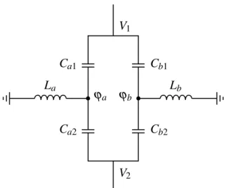
Ca1 Cb1
Ca2 Cb2
La Lb
V1
V2
ϕa ϕb
Figure 2.4:Device proposed to act as a high pass filter. It will allow to transmit pulses of two definite frequencies. A pulse coming from the transmission line 1 (V1) with frequency ωacan excite the oscillator in the branchaand be transmitted into transmission line 2 (V2). If the incoming photon has frequency ωb the same will happen with the other branch,
whereas if the frequency is neitherωanorωb, the pulse will not be transmitted.
On the other hand, when using a system of high pass LC filters like the one shown in FIG.2.4, with Hamiltonian
Hf = q
2 a
2(Ca1+Ca2)
+ q
2 b
2(Cb1+Cb2)+
Ca1V1+CaV2
Ca1+Ca2
qa+Cb1V1+CbV2
Cb1+Cb2 qb
−1
2
Ca1Ca2
Ca1+Ca2
+ Cb1Cb2
Cb1+Cb2
(V1+V2)2+ ϕ
2 a
2La
+ ϕ
2 b
2Lb, (2.23)
the resulting device has two levels that do not interact with each other. Since it does not contain a transmon inside, the lifetime of the excitations is small and the photons are transmitted fast. Nevertheless, there is a drawback in this system when compared to the transmon: in the transmon there is only one flux, whereas here there are two. Two fluxes mean two “artificial atoms”. Two more atoms that have to be coherently coupled to the rest of the system.
2.5
An alternative solution
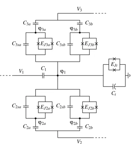
two-level atoms††. In both cases there are lots of possible excited levels –coming from the large number of fluxes and the large number of levels per atom– and thus, lots of sources of decoherence. Moreover, if I introduce these extra elements, the Hamiltonian will be modified, yielding a system where a photon has to interact with many elements before it can be transmitted and, probably, other processes that destroy the information contained in the photons may emerge from this new Hamiltonian. In order to simplify the system but introducing some elements that guarantee the proper operation of the quantum switch I propose a slightly differ-ent design from that of FIG. 2.2. Instead of two multilevel SQUIDs I use four modified high-pass filters. These elements, containing Josephson junctions in-stead of coils, are two-level SQUIDs. The new system is shown in FIG.2.5. This reduction of the levels of the SQUIDs drastically reduces the amount of possible interactions between the different energy levels that give, as an output, an out-going photon with the “wrong” energy (i.e., an outout-going photon with an energy different from that of the incoming photons. The device should not change the energy of the photons).
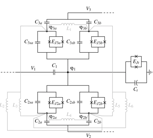
This device contains one multilevel transmon with a non-linear capacitor and four two-level SQUIDs. This translates into a flux with three excitations and four more fluxes with just one excitation each, as will be shown in Section3.1.
With this setup, when a photon is absorbed by the transmon, the energy levels of the filters are modified due to the Josephson elements in the SQUIDs. With regular inductors this would not happen because their energy do not contain high enough powers of the fluxes involved in this interaction, as it is the case for the SQUIDs [28–30]. I expect that when a second photon comes in –after the first is absorbed by the transmon and the energy levels of all the SQUIDs are modified–, it excites the only SQUIDd available and is decays into one of the outgoing trans-mission lines. Since these SQUIDs are two-level systems, the information carried by the photons will not be lost by the same mechanism as it was with the previous design (see Section2.3).
Now let us analyze the Hamiltonian for this device (FIG.2.5). The Lagrangian
††Transmons and SQUIDs are always multilevel systems. Whenever the wordmultilevelis used,
V1 C1 ϕ1
EJt
Ct
C3sa EJ3a C3sb EJ3b
ϕ3a ϕ3b
C3a C3b
V3
V2
C2sa E C2sb
J2a EJ2b
ϕ2a ϕ2b
C2a C2b
from which the Hamiltonian is derived is
L=C2a
2 (ϕ˙2a−V2)
2+C2b
2 (ϕ˙2b−V2)
2+C3a
2 (ϕ˙3a−V3)
2+C3b
2 (ϕ˙3b−V3)
2
+C2sa
2 (ϕ˙1−ϕ˙2a)
2+C2sb
2 (ϕ˙1−ϕ˙2b)
2+C3sa
2 (ϕ˙1−ϕ˙3a)
2+C3sb
2 (ϕ˙1−ϕ˙3b)
2
+C1
2 (ϕ˙1−V1)
2+Ct
2 ϕ˙
2
1+αtϕ˙14
+EJtcos
ϕ1
ϕ0
+EJ2acos
ϕ1−ϕ2a
ϕ0
+EJ2bcos
ϕ1−ϕ2b
ϕ0
+EJ3acos
ϕ1−ϕ3a
ϕ0
+EJ3bcos
ϕ1−ϕ3b
ϕ0
. (2.24)
The time derivative of the fluxes as a function of the momenta are
˙
ϕ2a=
p2a+C2aV2+C2saϕ˙1
C2a+C2sa
˙
ϕ2b=
p2b+C2bV2+C2sbϕ˙1
C2b+C2sb , (2.25) with a similar expression for ˙ϕ3aand ˙ϕ3b, and
˙
ϕ1=
21/3γ
f(x) −
f(x)
21/3β, (2.26)
with
γ =C1+Ct+
C2aC2sa
C2a+C2sa+
C2bC2sb C2b+C2sb+
C3aC3sa
C3a+C3sa+
C3bC3sb
C3b+C3sb (2.27)
β =6Ctαt (2.28)
x=p1+C1V1+ C2sa
C2a+C2sa
(p2a+C2aV2) + C2sb
C2b+C2sb(p2b+C2bV2)
+ C3sa
C3a+C3sa(p3a+C3aV3) +
C3sb
C3b+C3sb(p3b+C3bV3) (2.29)
f(x) =
−3β2x+
q
4β3γ3+ (3β2x)2
1/3
. (2.30)
These expressions are similar to the ones found before, so a similar Hamilto-nian is expected. Previously I had to expand the flux ˙ϕ1in a power series ofxup
and the excitation of the SQUID 2bplays the role of thesecond excitation– I only need to expand the flux up toO(x8). The Hamiltonian, up to this order, reads
H=−C1V 2 1
2 +
p22a+2p2aC2aV2−C2saC2aV22
2(C2a+C2sa)
+ p
2
2b+2p2bC2bV2−C2sbC2bV22
2(C2b+C2sb)
+ p
2
3a+2p3aC3aV2−C3saC3aV32
2(C3a+C3sa)
+p
2
3b+2p3bC3bV3−C3sbC3bV32
2(C3b+C3sb)
+ x
2
2γ − βx4
12γ4+ β2x6
18γ7− β3x8
18γ10−EJtcos
ϕ1
ϕ0
−EJ2acos
ϕ1−ϕ2a
ϕ0
−EJ2bcos
ϕ1−ϕ2b
ϕ0
−EJacos
ϕ1−ϕ3a
ϕ0
−EJ3bcos
ϕ1−ϕ3b
ϕ0
. (2.31)
This Hamiltonian has to be expanded, as before, in powers of the momenta to extract all the relevant interactions. To expand Eq. (2.31) I have imposedC2a>
C2sa and the same for the other three SQUIDs. I have also madeC1 small, but
not necessarily as small asCs2a. Previously I kept some powers ofCs2/(C2+Cs2)
because they were multiplying some expressions in the Taylor expansion of the Hamiltonian in Eq. (2.16) that I had to keep in order to give rise to interactions be-tween higher SQUID energy levels, although these factors (and their powers) were small. Now I can be more strict and get rid of all the terms of order (C2aC2sa+C2sa)3
or smaller because now the SQUIDs are two-level systems. Taking into account these considerations, the Hamiltonian can be separated in seven different expres-sions, which I now discuss
H1=
p21
2γ − βp41
12γ4+ β2p61
18γ7
+1
2
1+ C
2 2sa (C2a+C2sa)γ
p22a
C2a+C2sa
+1
2
1+ C
2 2sb (C2b+C2sb)γ
p22b
C2b+C2sb
+1
2
1+ C
2 3sa (C3a+C3sa)γ
p2
3a
C3a+C3sa+ 1 2
1+ C
2 3sb (C3b+C3sb)γ
p2
3b
C3b+C3sb
−(EJt+EJ2a+EJ2b+EJ3a+EJ3b)cos
ϕ1
ϕ0
−EJ2acos
ϕ2a
ϕ0
−EJ2bcos
ϕ2b
ϕ0
−EJ3acos
ϕ3a
ϕ0
−EJ3bcos
ϕ3b
ϕ0
H1 [Eq. (2.32)] contains information about the energy of the transmon and SQUID excitations. Just as before, the cosines have been separated and sorted into the different expressions that form the Hamiltonian.
The coupling between the different levels is contained inH2.
H2=
∑
k3
∑
i=1
A0ikp21ip2k−EJk
cosϕ1
ϕ0
−1 cosϕk
ϕ0
−1
!
, (2.33)
wherek∈ {2a,2b,3a,3b}. The reader is referred to AppendixB(SectionB.2) for a complete definition of all the coefficients in this expression.
The SQUIDs have to be coupled to the transmission lines. Actually they are coupled to all the transmission lines but, as expected, they are strongly coupled only to their nearest transmission line, whereas the transmon is weakly coupled to all the transmission lines. This makes its lifetime larger. This is expressed in the HamiltonianH3:
H3=
3
∑
i=1
B0i1Vip1+B0i3Vip31+
∑
kB0ikVipk
!
, (2.34)
with the coefficientsB0ikalso found in the aforementioned Appendix. The Hamil-tonian also contains some terms that describe the exchange of excitations between the transmon and the SQUIDs (H4) and also between the SQUIDs (H4.2):
H4=
1
γp1− β
3γ4p
3 1+
β2
3γ7p
5 1
C2sa
C2a+C2sap2a
−EJ2asin
ϕ1 ϕ0 sin
ϕ2a
ϕ0
+{2a→2b, 3a, 3b}, (2.35)
H4.2=
C2sa
C2a+C2sa
C2sb C2b+C2sb
p2ap2b
γ +
C3sa
C3a+C3sa
C3sb C3b+C3sb
p3ap3b
γ
+ C2sa
C2a+C2sa
C3sb
C3b+C3sb
p2ap3b
γ +
C3sa
C3a+C3sa
C2sb
C2b+C2sb
p3ap2b
γ
+ C2sa
C2a+C2sa
C3sa
C3a+C3sa
p2ap3a
γ +
C2sb C2b+C2sb
C3sb C3b+C3sb
p2bp3b
γ . (2.36)
After quantizingH4and alsoH4.2(see AppendixA), terms would appear
By choosing a suitable set of values for the energy of the Josephson junctions it is possible to make H4 vanish. In order to cancel also H4.2, more Josephson
junctions –or just regular inductors– have to be introduced into the system. It is trivial to introduce them in the Hamiltonian because their energy does not depend on the derivative of the fluxes, and they do not create other interactions: these extra elements only cancel H4.2 and increase the energy levels of the SQUIDs, slightly.
There are two more expressions that cannot be canceled but their contribution to the Hamiltonian is not much important, in contrast to the equivalent expressions for the previous device, from Section2.3. These areH5, in Eq. (B.2), andH6, in Eq. (B.3), both in the AppendixB.
H5 describes exchange of excitations between SQUIDs in the presence of an excited state in the transmon. This expression cannot be canceled in the same way asH4.2. It is of the same order asH2, but by comparing it withH3it can be seen that the excited SQUID will emit a photon into the transmission line rather than decay into another SQUID excitation. RegardingH6, it describes two processes: the relaxation of a SQUID excited state with the emission of a photon into any transmission line in the presence of an excitation in the transmon and the relax-ation of a SQUID state with the emission of a photon into a transmission line plus the excitation of two transmon energy levels. The amplitude of these processes is much smaller than those described inH3, so these are not likely to happen. Also because of the discrete energy separation of the transmon and SQUID levels, not all the combinations that appear in these two Hamiltonians are possible, especially if the energy spectrum of the transmon and the SQUIDs dissuade such processes to happen.
The advantages of working with this design are that all the necessary interac-tions are contained inH2 and H3, and that the contributions ofH5 andH6 to the
The Hamiltonian of these extra inductors is‡‡
Hi=1
2ϕ
2 3a
1 L1
+ 1
L2
+ 1
L3
+1
2ϕ
2 3b
1 L1
+ 1
L5+ 1 L6
+1
2ϕ
2 2a
1 L3
+ 1
L4
+ 1
L6
+1
2ϕ
2 2b
1 L2
+ 1
L4
+ 1
L5
−ϕ3aϕ3b
L1
−ϕ3aϕ2b
L2
−ϕ3aϕ2a
L3
−ϕ2aϕ2b
L4
−ϕ3bϕ2b
L5 −
ϕ3bϕ2a
L6 . (2.37) Now that all the necessary elements that form the quantum switch have been iden-tified and that the Hamiltonian contains all the desired interactions, it can be quan-tized and conditions can be imposed on the still free parameters that are left to cancel the remaining undesired interactions. This will result in a functional model for a quantum switch: the central element for a quantum random access memory based on circuit-QED.
‡‡The energy of an inductor with inductance L is 1
2∆ϕ2/L, where∆ϕ is the flux across the
V1 C1 ϕ1
EJt
Ct C3sa EJ3a C3sb EJ3b
ϕ3a ϕ3b
C3a C3b
V3
V2 C2sa E C2sb
J2a EJ2b
ϕ2a ϕ2b
C2a C2b
L2 L3
L4
L5 L6 L1
Chapter
3
Analysis of the model and further
considerations
The device schematically drawn in FIG.2.6 is the definitive design for the quan-tum switch. This device gives rise to the desired interactions, described by H1, H2 and H3 but it also produces processes that are unacceptable in a successfully operating quantum switch and, thus, have to be eliminated. These areH4,H4.2,H5
andH6. The last two expressions both contain exchange interactions. Compared to the other expression that contains this kind of interactions, the HamiltonianH3, the expressions in H5 and H6 describe very weak processes –the coefficients in front of each of the momenta are small, so these expressions lead to processes whose probability to happen are very small– and, thus, can be neglected. The way to deal with H4 and H4.2 consists of quantizing the Hamiltonian and imposing
the necessary conditions on the free parameters (Josephson energies, capacitances and inductances) to make these expressions cancel.
3.1
Quantizing the Hamiltonian
The procedure for quantizing the Hamiltonian is the usual: impose [pi,φi] =
i¯h/ϕ0∗ and cancel the expressions that should be canceled: the HamiltoniansH4
and H4.2 need to be strongly suppressed, so the only remaining expressions are
H1, H2 andH3. From these conditions the expressions for the momenta and the fluxes as a function of ladder operators are found. The fluxφ1and the momentum
∗The variables
p1read
p1=−
ih¯ 2ϕ0
3 2
γ2
βET
1/4
(a1−a†1) (3.1)
φ1=
2 3
βET
γ2
1/4
(a1+a†1), (3.2)
withET = h¯2
8γ ϕ02. The ladder operatorsa1anda †
1annihilate and create an excitation
in the transmon. The other fluxes and momenta are defined as
p2a=−
i¯h 2ϕ0
"
EJ2a
C2a+C2sa
C2sa
β
6γ2ET
1/2#1/2
(a2a−a†2a) (3.3)
φ2a=
"
1 EJ2a
C2sa
C2a+C2sa
6γ2ET β
1/2#1/2
(a2a+a†2a), (3.4)
with similar expressions forp2b,p3a,p3band the rest of the fluxes. In each of these
pairs of equations, the ladder operatorsa2a (and alsoa†2a) act on the SQUID that containsϕ2a. With this transformation, the terms inH4[see Eq. (2.35)] containing
a†a vanish, whereas the terms containing aa anda†a† disappear by making use of the rotating wave approximation. Now considerH4.2[displayed in Eq. (2.36)] together withHi [in Eq. (2.37)]. In order to cancel them, the extra inductances must satisfy†
L1= 4γ ϕ
4 0
EJ3aEJ3b 6γ2ET
¯ h2β
L2= 4γ ϕ
4 0
EJ3aEJ2b 6γ2ET
¯ h2β
L3= 4γ ϕ
4 0
EJ3aEJ2a
6γ2ET
¯ h2β
L4= 4γ ϕ
4 0
EJ2aEJ2b
6γ2ET
¯ h2β
L5=
4γ ϕ04
EJ3bEJ2b 6γ2ET
¯ h2β
L6=
4γ ϕ04
EJ3bEJ2a 6γ2ET
¯ h2β
. (3.5)
Once H1 has been expanded using these equations, the resulting expression
contains terms witha†a, but alsoa2, a2a†a, a4and higher orders ofa. Since it is not possible to get rid of all terms that do not conserve energy –interactions of the
†Boxed equations contain the conditions that must be imposed to the different parameters, i.e.,
kindaa,(a†)3a, etc–, the energies of the Josephson junctions have to be modified until some terms cancel and others become negligible. What can be canceled are the terms containinga2(and their hermitian conjugates). Consider the expressions inH1that contain information about the first energy level of the transmon. That is (the cosines have been expanded in a Taylor series), see Eq. (2.32),
H1.1=p
2 1
2γ +
¯ EJφ
2 1
2 , (3.6)
where ¯EJ =EJt+EJ2a+EJ2b+EJ3a+EJ3b. Expressed in the ladder operators, this becomes
H1.1=−
3 2
γ2
β ET
1/2
(a1−a†1)2+
E¯2 J
6
β
γ2ET
1/2
(a1+a†1)2. (3.7)
By using Josephson energies that satisfy the condition
¯ EJ =3γ
2
β , (3.8)
the expression forH1.1 becomes a simpler equation containing only a particle density operator
H1.1=2p2 ¯EJET a†1a1. (3.9) The same procedure has to be applied to the other elements in H1. After expanding them, some of the terms must be rearranged, since they may contribute to e.g. H1.1. These other expressions become
H1.1=
2p2 ¯EJET −7ET+90ET
r
2ET
¯ EJ
a†1a1, (3.10)
H1.2≈ −
7 2ETa
† 1 2
a21+90ET
r
2ET
¯ EJ a
† 1 2
a21
+5
3ET
a†1a1
a21+a†12
a†1a1
+5
2ET
a21+a†12
, (3.11)
H1.3≈ET
r
2ET
¯ EJ
20a†13a31
−45a†12+a21
−75a†1a1
a21+a†12
a†1a1
−15a†12a21
a21+a†12
a†12a21
In all these expressions I already got rid of some terms that contained high powers ofaand a†. In order to apply the rotating wave approximation, the pre-factor of aa has to be smaller than the prefactor of a†a. It can be achieved by imposing ¯EJ >ET. This implies thatCt is smaller than the other capacitances or that√αt h¯/ϕ0is small compared toγ.
These simplifications and approximations result in an expression forH1, the Hamiltonian that describes the energy levels of the transmon and SQUIDs, that only contains particle density operators (a†aand powers of this operator).
H1=
2p2 ¯EJET−7ET +90ET
r
2ET
¯ EJ
a†1a1
+ 90ET r 2ET ¯ EJ −
7 2ET
a†12a21+20ET
r
2ET
¯ EJ a
† 1 3
a31
+ 4pEJ2aE2a 2 ¯EJET +2
EJ2aC2sa
C2a+C2sa
2ET
¯ EJ
1/2!
a†2aa2a
+ 4pEJ2bE2b 2 ¯EJET +2
EJ2bC2sb C2b+C2sb
2ET
¯ EJ
1/2!
a†2ba2b
+ 4pEJ3aE3a 2 ¯EJET
+2 EJ3aC3sa C3a+C3sa
2ET
¯ EJ
1/2!
a†3aa3a
+ 4pEJ3bE3b
2 ¯EJET
+2 EJ3bC3sb C3b+C3sb
2ET
¯ EJ
1/2!
a†3ba3b, (3.13)
where the energiesE2a,E2b,E3aandE3bare
E2a=
¯ h2
8C2saϕ02
E2b= h¯
2
8C2sbϕ02
E3a= h¯
2
8C3saϕ02
E3b= h¯
2
8C3sbϕ02
. (3.14)
Unlike in the case of the flux φ1 and momentum p1, for the SQUIDs it is
EJ2aE2a= (E¯J−EJ2a+EJ2b+EJ3a+EJ3b)
ETC2sa
C2a+C2sa
EJ2bE2b= (E¯J+EJ2a−EJ2b+EJ3a+EJ3b) ETC2sb
C2b+C2sb
EJ3aE3a= (E¯J+EJ2a+EJ2b−EJ3a+EJ3b)
ETC3sa
C3a+C3sa
EJ3bE3b= (E¯J+EJ2a+EJ2b+EJ3a−EJ3b) ETC3sb
C3b+C3sb
. (3.15)
Now, ideally, EJ2a∼EJt so the SQUIDs and the transmon have similar en-ergy levels, but this equations tells thatEJ2a, EJ2b, EJ3a, EJ3b<<EJt –recall that
C2sa
C2a+C2sa <1.
Now I check whether these conditions are consistent with what is expected fromH2. This Hamiltonian contains the coupling between the transmon and the SQUIDs. Since all the couplings have the same form, by analyzing one of them the whole Hamiltonian can be easily found. Let me first study the coupling between the transmon and the SQUID 2a:
H2.1= −16ϕ 4 0ET2
¯ h4E¯J
p21+15·2
8
ϕ06ET3
¯
h6E¯J2 p
4 1−
42·212ϕ08ET4
¯
h8E¯J3 p
6 1
!
C2sa
C2a+C2sa
2
p22a
−EJ2a
φ12
4 −
φ14
48+
φ16
1440
φ22a. (3.16)
Now ladder operators could be plugged inside the fluxes and momenta using Eq. (3.1) to (3.4), but it can be simplified if all the six terms are compared by pairs. Let us consider first the terms in Eq. (3.16) containing p21p22aandφ12φ22a.
−16ϕ
4 0ET2
¯ h4E¯J
C2sa C2a+C2sa
2
p21p22a=−ETEJ2a
2 ¯EJ
C2sa C2a+C2sa
a1−a†1
2
a2a−a†2a
2
,
(3.17)
−EJ2a
4 φ
2
1φ22a=−
ET
2
C2sa
C2a+C2sa
a1+a†1
2
a2a+a†2a
2
.
(3.18)
analysis of the other four terms yields
H2.1≈ −
1−
180EJ2a ¯ EJ +
1 2
r
2ET
¯
EJ +7560
ETEJ2a ¯ EJ2
2ETC2sa
C2a+C2saa
† 1a1a
† 2aa2a
+
90EJ2a ¯ EJ +1 4 r 2ET ¯ EJ
+7560ETEJ2a ¯ EJ2
2ETC2sa
C2a+C2saa
† 1 2
a21a†2aa2a
−1680ETEJ2a ¯ EJ2
2ETC2sa
C2a+C2saa
† 1 3
a31a†2aa2a. (3.19)
To obtain this expression I have also used the rotating wave approximation. The full interaction Hamiltonian H2 is constructed by doing the same analysis with the other SQUIDs.
Up to this point, the only free parameters that are left are the capacitances, all of them, but with the constraintsC2a∼C2b ∼C3a∼C3b, C2sa∼C2sb ∼C3sa ∼
C3sb andCt, C2a >C1 >C2sa. The parametersV1, V2 andV3 are also still free
but in principle, in order to make the system scalable, they have to be equal. Nevertheless, I will assume that they can be slightly different –to check whether the system can be improved by not making it scalable– and at the end of the calculations, if it is possible, they will be made equal. For these potentials I have assumed the following quantized form
V1=− i¯h
2ϕ0
A11/4(b1−b†1) (3.20)
V2=− i¯h
2ϕ0
A12/4(b2−b†2) (3.21)
V3=− i¯h
2ϕ0
A13/4(b3−b†3). (3.22)
To derive the quantized form of the HamiltonianH3as a function of the ladder
operators I have also used the rotating wave approximation.The final expression reads
H3= 3
∑
i=1
µ1a,i−3µ1b,i
a†1b1+3µ1b,1a†1a†1a1b1
+µ1b,1a†1 3
b1+
∑
kµk,ia†kbi
!
+h.c. (3.23)
Here the indexkruns over{2a,2b,3a,3b}. The most relevant coefficientsµi,jthat
![Figure 1.1: A common random access memory can be schematically represented with this diagram [14]](https://thumb-us.123doks.com/thumbv2/123dok_us/8315218.2202908/9.892.122.707.196.404/figure-common-random-access-memory-schematically-represented-diagram.webp)