Modeling the Excess Cell Surface Stored in a
Complex Morphology of Bleb-Like Protrusions
Maryna Kapustina1☯*, Denis Tsygankov2,3☯, Jia Zhao4☯, Timothy Wessler5, Xiaofeng Yang4, Alex Chen5¤a, Nathan Roach1¤b, Timothy C. Elston3, Qi Wang4‡*,
Ken Jacobson1,6‡*, M. Gregory Forest5,7‡*
1Department of Cell Biology and Physiology, University of North Carolina School of Medicine, Chapel Hill, North Carolina, United States of America,2Wallace H. Coulter Department of Biomedical Engineering at Georgia Institute of Technology and Emory University, Atlanta, Georgia, United States of America,
3Department of Pharmacology, University of North Carolina School of Medicine, Chapel Hill, North Carolina, United States of America,4Department of Mathematics, University of South Carolina, Columbia, South Carolina, United States of America,5Department of Mathematics, University of North Carolina at Chapel Hill, Chapel Hill, North Carolina, United States of America,6Lineberger Comprehensive Cancer Center, University of North Carolina School of Medicine, Chapel Hill, North Carolina, United States of America, 7Departments of Applied Physical Sciences and Biomedical Engineering, University of North Carolina at Chapel Hill, Chapel Hill, North Carolina, United States of America
☯These authors contributed equally to this work.
¤a Current address: Risk Analytics Laboratory, GE Global Research Center, Niskayuna, New York, United States of America
¤b Current address: Department of Biology; Program in Cellular, Molecular, and Developmental Biology and Biophysics; Johns Hopkins University, Baltimore, Maryland, United States of America,
‡QW, KJ, and MGF also contributed equally to this work.
*[email protected](MK);[email protected](QW);[email protected](KJ);
[email protected](MGF)
Abstract
Cells transition from spread to rounded morphologies in diverse physiological contexts including mitosis and mesenchymal-to-amoeboid transitions. When these drastic shape changes occur rapidly, cell volume and surface area are approximately conserved. Conse-quently, the rounded cells are suddenly presented with a several-fold excess of cell surface whose area far exceeds that of a smooth sphere enclosing the cell volume. This excess is stored in a population of bleb-like protrusions (BLiPs), whose size distribution is shown by electron micrographs to be skewed. We introduce three complementary models of rounded cell morphologies with a prescribed excess surface area. A 2D Hamiltonian model provides a mechanistic description of how discrete attachment points between the cell surface and cortex together with surface bending energy can generate a morphology that satisfies a pre-scribed excess area and BLiP number density. A 3D random seed-and-growth model simu-lates efficient packing of BLiPs over a primary rounded shape, demonstrating a pathway for skewed BLiP size distributions that recapitulate 3D morphologies. Finally, a phase field model (2D and 3D) posits energy-based constitutive laws for the cell membrane, nematic F-actin cortex, interior cytosol, and external aqueous medium. The cell surface is equipped with a spontaneous curvature function, a proxy for the cell surface-cortex couple, that isa
prioriunknown, which the model“learns”from the thin section transmission electron micro-graph image (2D) or the“seed and growth”model image (3D). Converged phase field
OPEN ACCESS
Citation:Kapustina M, Tsygankov D, Zhao J, Wessler T, Yang X, Chen A, et al. (2016) Modeling the Excess Cell Surface Stored in a Complex Morphology of Bleb-Like Protrusions. PLoS Comput Biol 12(3): e1004841. doi:10.1371/journal. pcbi.1004841
Editor:Qing Nie, Irvine, UNITED STATES
Received:September 16, 2015
Accepted:March 1, 2016
Published:March 25, 2016
Copyright:© 2016 Kapustina et al. This is an open access article distributed under the terms of the Creative Commons Attribution License, which permits unrestricted use, distribution, and reproduction in any medium, provided the original author and source are credited.
Data Availability Statement:All relevant data are within the paper and its Supporting Information files.
Funding:This work was supported by NSF-DMS-1200487 (QW), AFOSR-FA9550-12-1-0178 (QW), an SC EPSCOR/IDEA award (QW), NSF-DMS-1200535 (KJ, QW, MK), NIGMS R01 GM078994 (KJ, TCE, MGF and MK ), NSF DMS-1100281(MGF). The funders had no role in study design, data collection and analysis, decision to publish, or preparation of the manuscript.
simulations predict self-consistent amplitudes and spatial localization of pressure and stress throughout the cell for any positedstationarymorphology target and cell compart-ment constitutive properties. The models form a general framework for future studies of cell morphological dynamics in a variety of biological contexts.
Author Summary
Individual cells must have the capability for rapid morphological transformations under various physiological conditions. One of the most drastic shape transformations occurs during the transition from spread to rounded morphologies. When this transition occurs rapidly, there is insufficient time for significant changes in surface area to occur, although the final size of the rounded cell indicates a significant reduction in apparent cell surface area at light microscope resolution. By contrast, high-resolution scanning electron micro-graphs of rapidly rounded cells reveal that a large amount of surface area is stored in a highly convoluted surface morphology consisting of bleb-like protrusions (BLiPs) and other small structures that are unrecognizable at lower resolution. This surface reserve is an important part of the mechanism that allows rapid and efficient large scale transforma-tions of cell shape. Remarkably, although this convoluted morphology has been observed for decades, there has been very little effort recognizing and including this surface surplus in mathematical modeling of cell morphology and physiology. In this paper, we develop three complementary models to fill this void and lay the foundation for future investiga-tions of the mechanisms that drive cellular morphological dynamics.
Introduction
Cells maintain their structural integrity while being flexible enough to adopt a variety of shapes. In general, it is the cytoskeleton of eukaryotic cells that drives shape transformation leading to cell movement and provides the structural support to the cytoplasm and the means to resist external forces. The periphery of cells, consisting of the plasma membrane (PM) and the acto-myosin cortex, is highly dynamic to accommodate shape change. The plasma membrane (PM) consists of a high density of proteins [1] embedded in a phospholipid bilayer of 5–10 nm thick-ness, with a very limited ability to extend without rupture [2,3] but highly amenable to bending [4,5,6]. The thin (50–500 nm) layer of cytoskeleton structure immediately subjacent to the plasma membrane, known as the cell cortex, consists of a dense F-actin network that is cross-linked by actin binding proteins and is amenable to contractility mediated by myosin motors. Interposed between the cortex and the PM is a thin spectrin-actin network, forming a‘fishnet’ with a mesh size of ~100 nm [7,8]. This structure is anchored both to the PM and cortex by adaptor proteins. In the following, we term the plasma membrane and spectrin-actin network as the“cell surface”.
many shape transitions occurring in non-spread cells, in this paper we reconsider this hypothe-sis in context of one of the most drastic changes of cell shape: the transformation from a fully spread to a rounded state.
If a cell transitions from a spread to rounded state while maintaining a constant volume, it will experience an excess of surface area over the minimum needed to cover the enclosed vol-ume. Because this process typically happens rapidly (~30s-), there is insufficient time for excess membrane to be internalized by endocytosis. Thus, another mechanism for storing surface area at the plasma membrane must exist. Indeed, there is significant evidence from both elec-tron and fluorescence microscopy that during the rounding process the cell surface adopts a tightly folded morphology [9,10,11,12].
While there are a number of models for cell shape, most of them treat the cell surface as smooth [13,14,15,16,17] and do not take into account the possibility that rounded cells store excess surface area in a dense distribution of bleb-like protrusions (BLiPs). Thus, new modeling approaches are needed to understand the dynamics of cell shape changes that involve active use of this surface storage. We introduce three complementary modeling approaches, each incorporating the concept of excess surface area. The first approach is a 2D model based on a thin cell surface structure that is coupled to a thicker, contractile actomyosin layer. This model allows us to investigate the folding of the excess surface and to estimate the bending energy in different configurations. The second approach is a random“seed and growth”model that pro-duces 3D morphologies consistent with the distributions of BLiP size and number estimated from scanning electron micrographs. This model yields insight into how large numbers of BLiPs are efficiently packed on the cell periphery.
The third approach is a multi-compartment phase field model. By faithfully capturing the physical properties of the cortex, cytosol, and cell surface, the model predicts the stress and pressure distributions associated with a highly folded 2D morphology and a dense distribution of 3D BLIPs. Phase field models have been widely used to study complex systems comprised of distinct material phases and their adjacent interfaces. When the separate material phases are immiscible, the phase field approach is to prescribe a finite thickness of a“diffuse”interface within which there is a mixture of the two materials [18,19]. The phase field method is an alter-native to sharp interface methods; in both methods the shape and evolution of the sharp versus diffuse interface are part of the solution. For every pair of adjacent material components, a phase field variable is introduced that interpolates from one material phase to the other through the finite thickness boundary. Phase field models have been employed to describe shapes of lipid bilayer vesicles in which the surface tension and Helfrich bending energy are approximated using a bulk energy defined within the diffuse interfacial layer [19]. Phase field models have been applied to many interfacial problems including liquid drops, multiphase complex fluids [20], and fractures in solid-state materials [21].
The phase field model simulations achieve separate goals. From either a 2D transmission electron micrograph or a 3D image reconstruction of the cell morphology, the model“learns” the spontaneous curvature functional of the rounded, BLiP-rich, morphology. Since the phase field model faithfully captures material properties of each cellular compartment, the model converges to the cell target morphology while constructing self-consistent stress and isotropic pressure distributions for the cell surface, cortex and cytoplasm, as well as estimating the nematic orientation within the cortex.
distributions rather than relying on extensive membrane-cortex remodeling and exocytosis. Thus, the theoretical approaches presented here should be applicable in a number of different biological contexts.
Results
Cell rounding produces an accumulation of excess surface at the cell
periphery
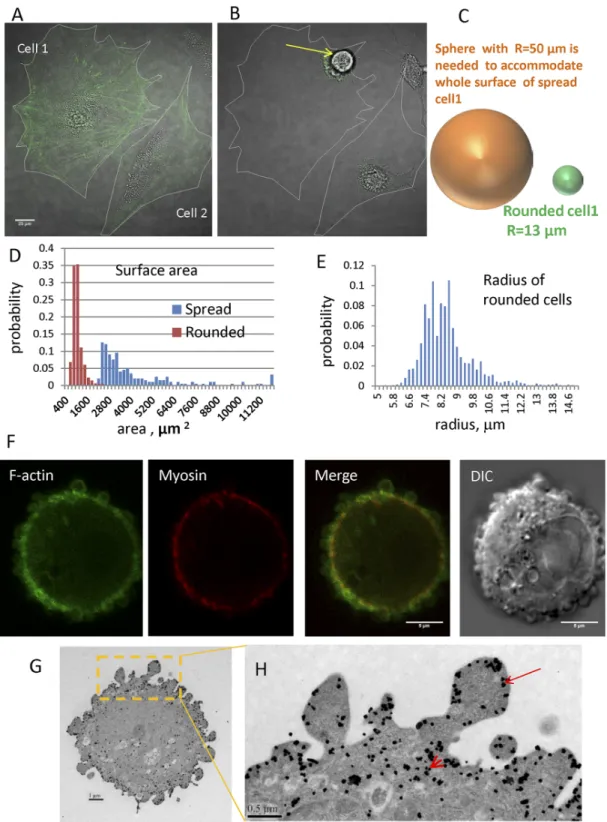
When spread cells (Fig 1A) are chemically detached from an underlying substrate, they rapidly transition to a rounded state on a characteristic time scale of ~30-60s (Fig 1B). Numerous stud-ies suggest that in media with constant osmolarity, cell volume is stable [3,22]. We estimated cell volume by reconstructing 3D geometries from Z-stacks of spinning disc fluorescence images of cells undergoing rounding. The mean volume for Chinese hamster ovary (CHO) cells in the spread state is 6.5±2.82103μm3, while the mean volume in the rounded state is 5.7 ±2.30103μm3, indicating a slight decrease in cell volume after rounding. Because this slight decrease in cell volume would only increase excess surface area, in all our models, we assume that cell volume remains constant during rounding.
The surface area of a spread cell is estimated as twice the area measured from images to account for dorsal and ventral surfaces. In reality cells are not completely flat and have more sur-face area due to finite thickness, particularly around the nucleus. Therefore, we are underestimat-ing the surface area of a spread cell. In the rounded state, the minimal surface area needed to enclose the measured cell volume can be found by assuming the cell is spherical and calculating the radius. For example, the cell 1 inFig 1Ahas a surface area of ~ 31000μm2while the surface area needed to enclose the rounded state is only ~ 2200μm2. Therefore after rounding, this cell has ~ 14 times more surface area than is required to enclose its volume. This image presents an extreme case of surface area excess. For cell 2 inFig 1A, which is less spread before detachment, an excess surface area of about five times the required amount is accumulated following round-ing. It is important to note that the amount of excess surface area that is accumulated during rounding depends on cell type and characteristics of the spreading and detachment for individual cells. Using DIC and fluorescence microscopy, we studied populations of cells before and after detachment, and individual cells rounding during trypsinization. The histogram inFig 1C pres-ents the distribution of surface areas for spread CHO cells (blue bars; population mean = 4310 ±3600μm2, N = 199) and cells immediately after rounding (red bars; population mean = 892 ±284μm2, N = 1646). The distribution of rounded cell sizes is narrow with majority of cell radii (Fig 1E) being between 7 and 9.5μm (mean = 8.36±1.24μm; N = 1646). Separate experiments, where we followed the change in morphology of individual cells during rounding, demonstrated that for CHO cells the average excess surface, defined as the ratio of spread cell area to that required to smoothly cover a sphere with radius corresponding to that of the rounded cell, accu-mulated due to detachment and rounding is 3.8± 2.06 with maximum value of 12 (N = 99).
To gain insight into how much excess surface area can be stored in BLiPs, we first consider the case of a rounded cell uniformly covered with equally sized sphererical BLiPs.
surface is dictated by a balance between the necessity to pack tightly a very large number of BLiPs and the necessity to generate, regulate, and maintain significant surface curvature.
Cortex architecture informs the 2D discrete geometric model
To better understand the process of packing cell surface excess into a convoluted surface mor-phology, we constructed a 2D geometric model designed to produce BLiPs. We hypothesize that the cell surface and underlying contractile cortex form a two-layer structure that is coupled at certain fixed points. The first layer, which we term the cell surface, is passive and consists of the plasma membrane and membrane associated cytoskeleton. This layer is assumed to be sim-ilar to the spectrin-actin network that is coupled to the plasma membrane of red cells [23]. Such structures have been shown by Kusumi and co-workers to exist in many other cell types [8]. The membrane associated cytoskeleton has been termed the membrane skeleton fence [8]. It is basically a very thin filamentous meshwork that provides a“fishnet”with a mesh size of approximately 100 nm immediately underlying the PM. This layer is coupled to the plasma membrane via adaptor proteins including the ankyrin and ERM families as well as by interac-tions of the membrane skeleton fence with lipids in the inner monolayer of the PM. The layer is thought to be passive undergoing only thermal motions, serving to anchor some transmem-brane proteins and restrict the free diffusion of others. We assume that this thin layer is cou-pled via adaptor proteins to a thicker, active contractile layer containing actin and myosin. This view of the cortex-cell surface couple is consistent with that advanced by Charras et al (2006) [24] in the context of spontaneously blebbing cells.
Additional evidence for this structure comes by imaging employing confocal and electron microscopy.Fig 1Fshows a confocal image of the actin-myosin cortex in rounded cells as visu-alized with GFP-lifeact and RFP-myosin merged with a DIC image of the same cell. The green signal for Lifeact marks F-actin filaments associated with the folded morphology of the cell periphery and this fluorescent signal originates from both the thin layer immediately subjacent to the membrane and the thicker contractile layer. The fluorescent signal from myosin (red) shows that this protein is localized mainly to a thin circle located below the BLiPs and more toward the cell interior.S1 Figpresents Z-stack images of the same cell. From this image, it is clearly visible that the convoluted morphology covers the whole cell.Fig 1G and 1Hshows immunogold TEM images of GFP-lifeact where F-actin is seen underlying BLiPs (arrow) and also in a layer closer toward the center of the cell (arrowhead).
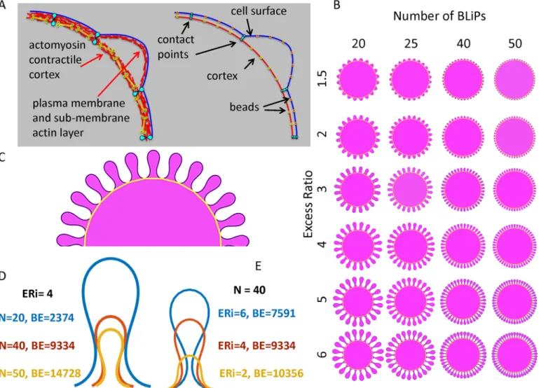
To construct the 2D geometric model introduced qualitatively above, we implement a two-layer architecture in a 2D bead-spring model of the cell membrane and cortex (model descrip-tion inMethods). The bead-spring model consists of two-layers (Fig 2AandS2 Fig), where one layer (outer layer) represents the membrane and underlying actin mesh (i.e. the cell surface) and the other layer (inner layer) represents the actomyosin-rich contractile cortex. In each layer, beads are connected pairwise by springs and contact points serve to connect the two lay-ers. By minimizing the bending energy we explored the steady-state shapes of BLiPs generated during cell rounding when the cell is rapidly presented with a substantial excess surface. For simplicity we define excess surface ratio (ER) as a ratio of perimeters of the surface layer and contracted cortex. Here we define a normalized total bending energy (E) as for
E¼
I
s
k2ds L
N
XN
i¼1 k2
i ð1Þ
The number of contact points determines the number of folds (M). In the simulation the total Hamiltonian of the two-layer system is minimized with the result that a folded configuration of outer layer is produced.Fig 2Bshows the resulting shapes as a function of bothMand ER.Fig 2Cshows a portion of a model cell with BLiPs at steady state where the gold line represents the contractile part of the cortex with contact points. While the appearance of folds is expected, the shape of folds and the bending energy stored in each configuration is of particular interest.
Fig 2Dgives a comparison of the fold configuration for several different sets of parameters with the calculated bending energy for each shape. Inspection of the fold shapes shows that in order to accommodate more surface, the folds tend to develop long necks. (Note that in case where there is heterogeneity in the size of folds, this effect would allow small folds to grow under larger ones, an effect that permits accommodation of more excess surface.) The smallest possible bending energy will be achieved when ER = 1 and M = 0 (no surface excess and no BLiPs). For a given value of ER, the energy increases with the number of BLiPs (Fig 2Dand
Fig 2. The discrete geometric model.A. Two layer cortex model (left) and its bead-spring representation with notations employed (right). B. Folded geometries as a function of the fold number and the excess surface ratio. C. A portion of a model cell with BLiPs at steady state where the gold line
represents the cortex. D. The shape of three single folds extracted from simulations for initial excess ratio, ER = 4 with different numbers of folds, N: 20 (blue), 40(red) and 50(yellow). E. The shape of three single folds extracted from simulations for number of folds N = 40 with different initial excess ratio, ER,: 6 (blue), 4 (red), 2 (yellow). All calculated shapes were scaled to have the same unit area inside the outer perimeter. The bending energy (BE) is presented for each configuration.
S2 Fig). However, the bending energy is decreasing while the excess surface ratio is increasing. Although this result looks counterintuitive, it can be explained. The local curvature is the inverse of local radius. Folds with a longer perimeter have bigger inner radii which substantially decreases bending energy with the square of local radius (Fig 2DandS3 Fig). Thus, morpholo-gies with longer perimeters corresponding to larger ERs will have lower energy compared to the shapes with the same number of folds but with shorter perimeters (i.e. smaller ERs). The analysis of the area which is stored inside the folds (i.e., volume in 3D) shows that for the same surface excess, more area is stored in folds when the number of folds used for accommodation of this surface surplus is smaller (S3D Fig).
BLiP size measurements
At the resolution achievable by standard fluorescence microscopy, the convoluted cell surface often appears as a thickening of membrane and cortical stains (Fig 3A and 3B). However,
Fig 3. Morphology of rounded cells.A. Fluorescence, DIC and merged images of rounded CHO cells stably transfected with Lifeact-GFP. B.
Fluorescence, DIC and merged images taken near the equatorial plane of a rounded CHO cell with the fluorescence signal coming from the PH domain of PLC-delta fused to EGFP that marks the inner leaflet of the plasma membrane (Bar = 5μm). C. Scanning electron microscope image of the rounded state (Bar = 5μm). D. BLiP radii distribution for N = 7096 BLiPs.
surface morphology can be imaged at higher resolution using both scanning (SEM) and thin-section transmission (TEM) electron micrographs (Figs3Cand1H, respectively). At this scale, bleb-like protrusions (BLiPs) and other cell surface protuberances are clearly visible. Note that only fully spread cells have a smooth surface essentially devoid of protrusions (S4 Fig).
To determine length, area and volume metrics of BLiPs, we manually segmented SEM images of cells that were fixed after rounding (S5 Fig). Each protrusion was approximated as a sphere and the area of the protrusion visible on the image was interpreted as a two dimensional projection of that sphere. We calculated the radius that corresponds to a projection of that size, and consider it as the radius of the BLiP. The distributions of BLiP radii derived from 10 SEM images (25 cells) that include 7096 BLiPs is presented inFig 3D. We find that the distribution of radii is skewed with a preponderance of small BLiPs and a decreasing frequency of larger BLiPs. The mean BLiP radius is R = 0.25μm with a median of 0.22μm and mode of 0.19μm.
It is important to mention that during the processes of detachment and rounding some part of the cell surface can be lost due to incomplete detachment from the substrate or because it remains in retraction fibers. However, the area remaining in retraction fibers is quite small. Using SEM images from cells that spread for 24 h and rounded 5 minutes before fixation, we estimated that the surface area that might be stored in retraction fibers represents between ~0.5–5% of the cell surface area in the spread state.
BLiP packing on the cell periphery
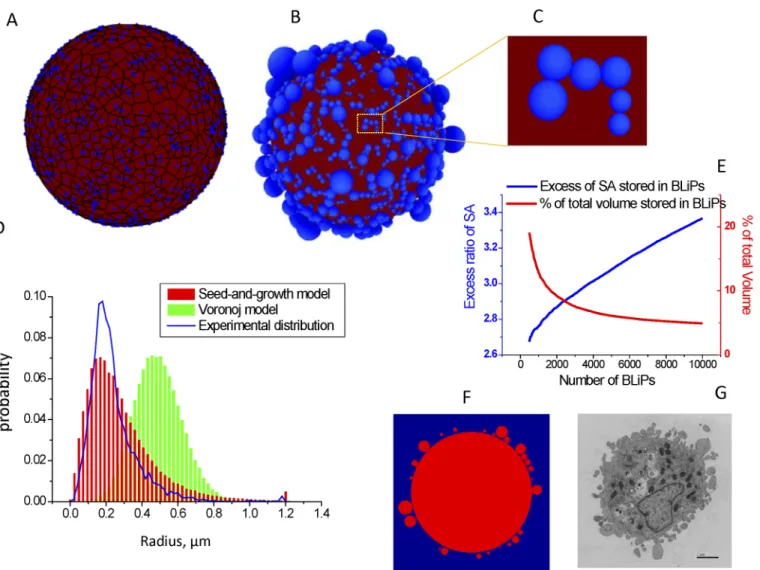
To investigate how the large number of BLiPs required to accommodate the excess cell surface are packed on the cell periphery, we constructed two models. As a plausible starting point, we employed a Voronoi approach, in which a spherical ball of radiusR¼pffiffiffiffiffiffiffiffiffiffiS=4pcontains the surface area, S of the spread cell before detachment and rounding;nseed point locations are randomly sampled from a uniform spatial distribution on the ball. The ball is then partitioned by a Voronoi tessellation according to thenseed points (Fig 4A) such that any point in each Voronoi cell is closer to the parent seed point than any other seed point. The area of each Voro-noi cell is then determined. In this configuration, we assumed that, upon the cell rounding to itsfinal state with the“BLiPed”morphology, each Voronoi cell of areavmorphs into a spheri-cal BLiP with radiusr¼pffiffiffiffiffiffiffiffiffiffin=4p.Fig 4Ddemonstrates that, constructed in this way, the distri-bution of BLiP radii has a well-defined length scale with the bell-shape distribution, which is not consistent with the skewed distribution of experimental data. This result arises from the fact that Voronoi cells corresponding to two very closely positioned seeds are not necessarily small themselves, as might be expected from two closely positioned BLiPs.
In order to mitigate this effect, we introduce an alternative 3D“seed and growth”model (Fig 4B and 4C), in which BLiP radii are proportional to spacing between randomly distrib-uted seeds. In this model, spheres are generated from each seed point by increasing their radii at a uniform rate. Simultaneously, the locations of the seed points are moved outward radially at the same rate, so that the spheres always remain tangent to the cell. When one sphere encounters another, it stops growing. When all spheres have stopped growth, a spherical cell coated by different sized BLiPs is produced (Fig 4B). The resulting BLiP radius distribution in
In the“seed and growth”model, a larger number of BLiPs results in a higher surface area excess ratio (Fig 4E) and a smaller percentage of the cell volume stored within the BLiPs, which is consistent with our simplified estimations based on an 2D equal-sized BLiP distribution. In principle, BLiPs that are not of equal size could allow a more efficient packing of excessive cell surface (with smaller BLiPs filling the space between larger ones), which is important for accommodating very high excess ratios (>5). However, in this model the packing is still ineffi-cient because it always generates areas devoid of BLiPs. A potential improvement to our model might be to incorporate stochastic seeding of new BLiPs and occasional“shrinking”BLiPs that are in contact, so that BLiPs are dynamic and continue to adjust themselves toward the most efficient filling of the available space. Such a“seed, growth, and shrinking”model would be consistent with the BLiP dynamics observed in our experiments, but is beyond the scope of the
Fig 4. BLiPs morphology generated by seed-and-growth models.A. A realization of the Voronoi diagram. The seeds and boundaries of Voronoi cells are shown in blue; the Voronoi polygons are shown in red. B. A realization of the“seed and growth”model. C. Magnified view of rectangle in (B). D. Distribution of BLiP sizes: Voronoi model (green bars) and“seed and growth”model (red bars) normalized using the assumption that average rounded cell radius is 8 um; the blue line shows the experimentally obtained distribution. E. For the“seed and growth”model, plots of % surface area stored in BLiPs and % of total volume stored in BLiPs as a function of the number of BLiPs. F. A cross-section of“seed and growth”model. G. Transmission electron micrograph of a section of a rounded cell (Bar = 2μm) for comparison to F.
current paper. Another potential improvement would be to make final BLiP size proportional to the rate of expansion of the BLiP; this has been found to be the case in an earlier study of blebbing cells [30].
A phase field model can learn the spontaneous curvature of the cell
surface from 2D transmission electron micrographs or 3D image
reconstructions
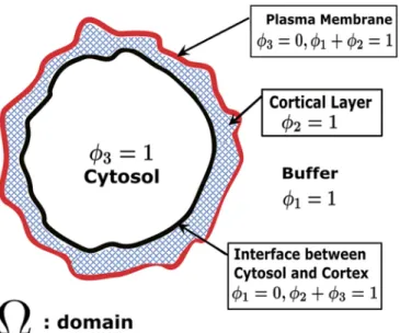
The preceding models help build mechanistic intuition, yet, while predictive, they do not cap-ture all of the essential physics of the rounded phenotype. In order to approach this goal, we formulated 2D and 3D phase field models for a cell immersed in the aqueous extracellular envi-ronment. The model is formulated in 3 space dimensions (3D), but it also restricts to 2D for purposes of modeling a cell cross-section. In our case, we have three phases (exterior aqueous medium, cortex, interior cytosol) and two diffuse interfaces. The external aqueous medium and interior cytosol are modeled as viscous fluids with specified viscosities and the cortex is modeled as a nematic (liquid crystal) gel [31]. The first diffuse (i.e., finite thickness) interface is what we have termed the cell surface, consisting of the plasma membrane and very thin under-lying filamentous“fishnet”, that separates the aqueous medium and the cortex proper. As described below in Methods, a particular level set function in the phase field formulation will afford our definition of the“cell surface”. The second diffuse interface is the cortex-cytosol transition layer.Fig 5is a 2D schematic of a 3D cell cross-section with individual components and diffuse interfaces labeled, along with the phase variables defined below. (We do not explic-itly model the nucleus within the cytoplasm for this paper since we are primarily concerned with the stationary rounded morphology.) A more complete mechanical formulation giving the total system free energy in terms of its components is found in Methods.
Fig 5. Schematic for the phase field formulation of a cell in an aqueous medium.ϕ1,ϕ2,ϕ3, represent volume fractions of the external aqueous medium, the nematic cortex as schematically depicted by the cross-hatched region and the cytosol, respectively, withϕ1+ϕ2+ϕ3= 1. The entire computational domain is denoted asΩ. The cell surface is defined by the level setsϕ1=ϕ2= 0.5, while the cortex-cytosol interface is defined by ϕ2=ϕ3= 0.5. Note that we penalize coexistence of three phases.
Phase field modeling of a 2D cell surface morphology with excess
“
perimeter
”
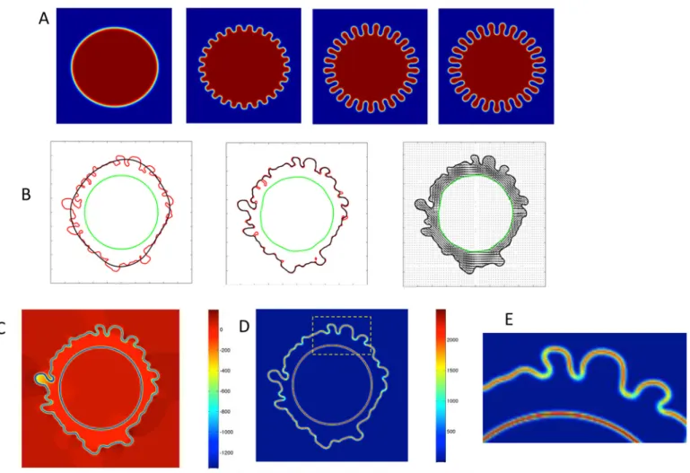
We summarize the key numerical results of the phase field modeling of a 2D cell surface mor-phology due to an imposed excess arc length enclosing the 2D area. We require a 2D image of the membrane morphology, taken from 2D transmission electron micrographs. From the image file, we posit an initial smooth membrane boundary, and then evolve the phase field model while adjusting the spontaneous curvature functionC1 until the model converges to the image dataset. We first illustrate the ability of the phase field model to match an arbitrary spec-ified 2D boundary by“learning”the spontaneous curvature function; the results are shown in
Fig 6Afor an illustrative benchmark in which the cell perimeter contains 25 regularly spaced, uniform“BLiPs”. (In 2D, this is achieved by superimposing the appropriate Fourier mode on a
Fig 6. Application of the phase field model to 2D target images.A. Proof of principle of the 2D phase field simulation. From left to right, convergence from circular initial data to a target cell surface morphology with 25 uniform, equally spaced,“BLiPs”. B. Convergence of a 2D phase field simulation to a 2D, TEM image of a representative cell surface morphology. The red curve in panels 1–3 is the cell surface obtained from a 2D TEM micrograph, which serves as the target of the phase field model. The black contours in each panel are the initial data (left panel) which evolves to the actual cell surface in the phase field simulation. The green contours depict the interface between the cortex and interior cytosol. In the right panel, the F-actin filament orientational distribution within the nematic cortex is superimposed, as predicted by the phase field model. In these simulations, the Flory order parameter,pffiffiffiffiffiffiffiffiffiffiffiffih1=h2, is set to 1. C. Phasefield predictions of the pressure distribution. D. thefirst invariant (trace) of the dominant stored stress, the Ericksen stress, for the converged stationary morphology shown in B, right panel. E. A blow-up of the trace of the Ericksen stress inside the dashed yellow rectangular domain in D. The color bars for C, D, and E are in units of Pascals.
circle.) Next, we used as input the actual periphery of a rounded cell from a 2D transmission electron micrograph (TEM) image. The results inFig 6Bshow the convergence of the phase field membrane morphology to the TEM image, where the nematic phase ordering (represent-ing F-actin orientation) in the cortex is depicted. This result assumes tangential anchor(represent-ing con-dition of F-actin at both cortical diffuse interfaces.
Fig 6C–6Eshows the phase field predictions of the pressure distribution (C) and the first invariant of the dominant stored stress, the Ericksen stress, for the converged stationary mor-phology (D,E) shown inFig 6B. These results reveal the orders of magnitude as well as spatial localization of pressure and stored stress for the target 2D morphology.
Phase field recapitulation of 3D BLiP morphologies and associated
stress maps
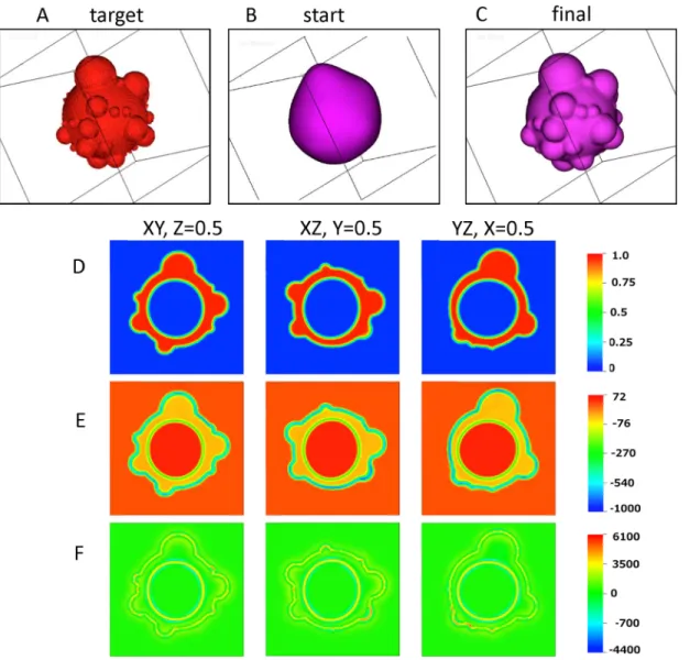
A 3D simulation is depicted inFig 7to demonstrate the capability of our phase field model to converge to atarget3D cell surface morphology. The excess surface area ratio for this illustra-tion iss0= 3. Because it is impossible to reproduce a full 3D morphology of a rounded cell from a single scanning electron micrograph, we use the“seed and growth”model to simulate a 3D cell surface target. This model (Fig 4) provides a 3D surface morphology consistent with the measured BLiP size distribution data; therefore, we posit the output image from this model as the target morphology for the 3D phase field simulation. As shown earlier in 2D and here in
Fig 7in 3D, the phase field model converges to the target 3D morphology from an initial pos-ited surface, while satisfying the volume and excess surface area constraints. The model does so by iterating the spontaneous curvature function until all constraints are satisfied; once con-verged, the model then yields the pressure and stresses within the cell surface and cortex that are self-consistent with the 3D surface morphology and constitutive properties of the exterior and cell compartments.
InFig 7A, the target cell morphology is shown. The evolution of cell morphology, from an initial rounded cell guess to the target cell shape, is provided in (Fig 7B and 7C).Fig 7Ddepicts 2D projections in three mutually orthogonal planes of the cell surface morphology as well as the cortical layer and interior cytosol domains, displaying the values of the phase field variables for each domain. InFig 7E and 7Fthe model predictions for hydrostatic pressure distributions and stored stress in the same orthogonal planar sections for the stationary morphology are given correspondingly. The pressure values are not unreasonable (e.g. a 1 mm depth of water at atmospheric pressure exerts a hydrostatic pressure of 9.8 Pa). The pressure is low and positive in the external aqueous medium and cytosol; therefore, an inward pressure is exerted from the external medium to the cell surface and an outward pressure from the cell interior (cytoplasm) to the cortex. The pressure is negative in the plasma membrane and cortical layer meaning that this layer experiences an inward compressive pressure from the external aqueous medium and cytosol. The highest (compressive) pressures arise in the cell surface“interphase”nearby high curvature BLiPs, with about an order of magnitude lower values within the cortical layer itself. These stationary pressure gradients suggest a propensity for fluid absorption from the exterior aqueous medium into the cortex phase and cell surface interface. It is important to note that our simulations assume a stationary morphology, and the pressure and stress distributions are a consequence of the stationary assumption. In reality, these morphologies are non-stationary, and in particular there is flow of the cytoplasm that fills the BLiPs. The new balance of pressure and stress will then dictate the directional flux and flow of the external aqueous medium and cytosol through the various cell compartments.
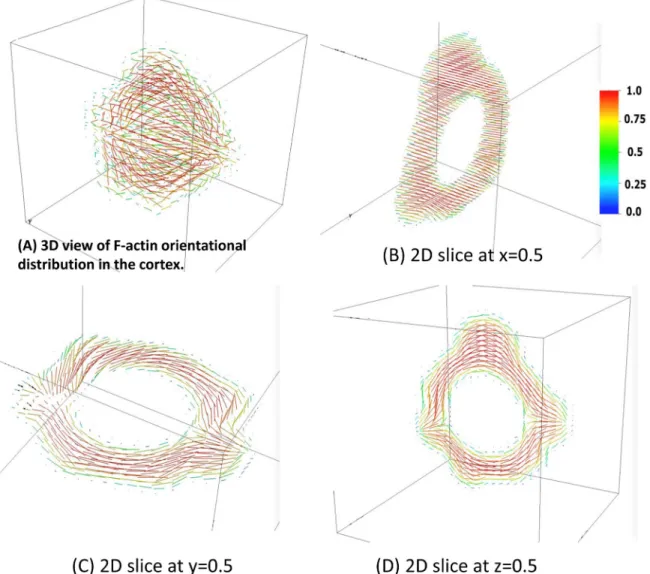
Fig 8B–8D. These figures convey the degree and direction of order within the F-actin filaments of the cortex, and their strong correlation with the cell surface morphology. Note that cortical F-actin is assumed to prefer parallel alignment at both cortical interfaces for this illustration of the 3D phase field model. The anchoring energy at the interfaces together with the presumed strength of the nematic potential are responsible for the relatively high degree of alignment of the F-actin; these parameters are tunable to match experimental data on nematic order within the cortex.
The nematic order was changed by varying Flory order parameter from 1 to values approaching 0. The results of these simulations are shown inS6 Figwhich shows the nematic order superimposed on the 3D morphology for order parameters that range from 1.0 to 0.01.
Fig 7. Phase field simulation showing convergence to a target 3D cell morphology image.(A) The target 3D cell morphology. (B) The assumed initial data for the cell surface. (C) The converged cell surface from the phase field simulation. (D) 2D planar slices at z = 0.5, y = 0.5 and x = 0.5, respectively, of the converged 3D phase field simulation shown in C. The color bar depicts level sets of the cortical phase variableϕ2to delineate the cortex (red is the level set ϕ2= 1) from the pure external aqueous medium and pure interior cytosol (both blue sinceϕ2= 0), while both diffuse interfaces are depicted by the color interpolation between these level sets ofϕ2. (E) Corresponding pressure distributions (units of Pa) in the 2D slices shown in (D). (F) Distribution of the trace of the Ericksen stress (units of Pa) in the 2D slices shown in (D). The color bar for E, F is in units of Pa. For these calculations the Flory order parameter is set to 1.
Cross-sections taken at three orthogonal planes are shown inS7 Fig. Note that the values assumed for K (the Franck elastic constant), and h1and h2will not significantly affect the
pres-sure or the Ericksen stress of the stationary morphology; this is because the dominant contribu-tion to the Ericksen stress is from spatial gradients of the level set funccontribu-tionϕ1= 1/2 that defines the cell surface. As shown inS6andS7Figs, h1and h2only affect the nematic order of the
sta-tionary state and K does not affect any of the predictions for the stasta-tionary morphology. How-ever, for dynamic processes, these parameter values will strongly dictate the results of the simulation.
Discussion
Using comparative measurements of many individual cells in two distinct configurations, spread on a substrate versus in a rounded state detached from the substrate, we showed that
the cell surface area in the rounded state is highly convoluted and far exceeds the surface area of a sphere that would enclose the volume of the cortex, cytosol and nucleus. We analyzed the size and distribution of bleb-like protrusions (BLiPs) on the cell periphery that served as stor-age for the excess of surface area. We then developed three complementary modeling approaches that incorporate the concept of excess surface area on rounded cells in different ways.
Employing a 2D discrete geometric model, we tested whether the two-layer composition of the cortex, with the outer layer termed the cell surface, giving the local shape of the BLiPs and the inner layer responsible for contraction, is sufficient to reproduce the highly folded surface observed after rounding. This model demonstrated that morphologies with longer perimeters corresponding to larger ERs will have lower energy compared to the shapes with the same number of folds but with shorter perimeters (i.e. smaller ERs). This result predicts that during cell rounding, larger folds, which are energetically more favorable, should appear early in the process. On the other hand, smaller folds will appear later because it can require time to build structures that will support the higher curvature folds. Indeed, several preliminary experiments in which cells are detached and imaged appear to support this notion. In the early stages of rounding, big folds often appear on the cell surface but, as time goes on, the cell breaks the large folds into the smaller ones. This is supported by the fact that we see a prevalence of small BLiPs in the distribution of fold sizes from the SEM and fluorescence imaging. It is also possi-ble that smaller BLiPs are required as the cell approaches a rounded, steady state because the large folds stored too much of the cell volume (S3D Fig) which could disrupt normal cell func-tioning. In addition, the ability to create smaller folds would be advantageous in storing large surface excesses in that small BLiPs could form under larger ones for more efficient packing.
Our 3D random“seed and growth”model of BLiPs approximated the BLiP number density and size distribution from 3D scanning electron micrographs. The model provided insight into the SEM image analysis that revealed skewed size distributions of the BLiPs, with a preponder-ance of small-scale features and successively fewer large-scale protuberpreponder-ances. Moreover, this model demonstrates that efficient packing of BLiPs requires that heterogeneity of BLiP sizes is needed to recapitulate 3D morphologies.
How do these three distinct approaches relate to one another? We postulate that cell surface regions rich in adaptor proteins bind the cell surface to the cortex, inheriting the mean curva-ture of the cortex. We have termed these regions attachment or contact points. Although the species composing these regions have not been identified, presumably they would belong to groups such as the ERM family of cytoskeletal-membrane adaptors as previously suggested in [24]. Moreover, one would expect that these contact points would be transient and regulatable leading to more dynamic behavior than we capture in the current models. Domains with less binding proteins allow the cell surface to detach from the contractile part of cortex forming BLiPs. We assume in our models that the distribution of binding protein species dictates the surface morphology, which in turn dictates the spontaneous curvature function. In the discrete geometric Hamiltonian model, the binding sites forming the attachments between the cell sur-face and the cortex are explicitly modeled, leading to an induced cell sursur-face morphology.
In the phase field model, we choose the level setϕ1= 0.5 to define and match the surface
morphology captured in 2D micrographs or reconstructed in 3D using the seed-and-growth model. Thus discrete Hamiltonian and phase field modeling approaches are complementary: the discrete Hamiltonian model is based on postulated attachment points that determine mor-phology, whereas the phase field model, in which specific molecular features are coarse-grained, is based on a spontaneous curvature function specific to and constructed from the morphology itself. In 3D, micrographs are not sufficient to provide a 3D image file due to sig-nificant occluded cell surface. Thus, we used images produced by seed-and-growth model that yields 3D images of the surface morphology that are statistically consistent with the measured 3D BLiP distribution data from scanning electron microscopy images. The phase field model then uses the 3D surface construction as an imposed target morphology, and the model evolu-tion adapts the spontaneous curvature funcevolu-tion until the target morphology is reached. The phase field model then predicts the stationary stresses and energies within the cell surface and cortex self-consistent with that surface morphology. It is important to note thestationary
aspect of the model predictions which identify stress contributions that are due to spatial gradi-ents of the fitted membrane morphology. Indeed, since the model simulation converges to the inputstationarymorphology, the stored stresses due to nematic elasticity all relax and are neg-ligible. I.e., the stress components are insensitive to the nematic parameters, and are dominated by the gradients of the level set functionϕ1= 0.5 learned from the morphology. The power of
the model will be further revealed when we investigate the dynamics of the highly convoluted morphology, where nematic parameters and constitutive properties of all compartments will then have significance. It will be important from a biological standpoint to learn the bounds on these parameters.
An additional caveat is that the models presented are purely mechanical or steric in nature. It is certainly possible that active processes other than cortical contraction, giving rise to corti-cal tension [32] during rounding could play a role even in the short time span of cell rounding from a spread state. For example, in our model, we did not include the actin polymerization process explicitly although but it is true that smaller BLiPs, which are the majority of the popu-lation, have higher bending energy so that they require stronger cortical support perhaps requiring additional actin nucleation and polymerization [33] on short time scales.
results presented here are derived for stationary BLiP-laden morphologies, these models form the foundation for future studies of cell surface dynamics regulated by coupling to reaction-dif-fusion kinetics of various molecular species. These kinetics can be expected to be controlled by signal transduction in many cases. The theoretical approaches presented here should find application in a number of different biological contexts.
Methods
Development of the discrete geometric model
The bead-spring model consists of two-layers (Fig 2A), where one layer (outer layer) represents the membrane and underlying actin mesh (i.e. the cell surface) and the other layer (inner layer) represents the myosin-rich contractile cortex. Within each layer, beads are connected pairwise by springs. Special contact points serve to connect the two layers via springs. At the beginning of simulation both layers have the same perimeter. During the simulation the inner layer (cor-tex) shrinks in order to reach the target enclosed area with smaller perimeter, imitating cortex contraction. The presence of contact points between two layers enforces outer layer bending (S2 Fig). Although the more correct definition of the excess surface ratio is
ε2D¼
L
2pR ¼L=2
ffiffiffiffiffiffiffiffiffiffiffiffi
pAtotal
p
, whereLis the perimeter of the surface layer andRis the radius of the circle that would enclose the area inside this surface layer (Atotal), for the simplicity we
define excess surface as a ratio between the perimeters of surface layer and contracted cortex. Let the surface layer with the perimeter L be represented byNbeads (S2 Fig), with the nota-tional convention that bead 0 corresponds to beadN(representing a closed contour). Then the Hamiltonian for this outer layer of beads and springs (i.e. the cell surface) is:
Hout¼c1SNi¼1k2i þc2S N
i¼1ðliL=NÞ
2; ð2Þ
wherekiis the local curvature of the surface at beadi;liis the length of the spring between beadsiandi+1; andc1andc2are free parameters that define relative contributions of the
energy terms. Thefirst term inEq 2is the energy cost for bending the surface layer. The second term ensures that the outer layer does not significantly stretch or contract during the simulated process.c1andc2are chosen withc2c1so that as the system approaches a steady (minimum
energy) state, thefirst term tends to a configuration that minimizes curvature and the second term tends to zero.
The Hamiltonian of the inner, contractile layer (i.e. the cortex) is:
Hinn¼c3SMj¼1p2j þc4ðAAÞ2; ð3Þ
whereMis the number of beads in the inner cortex (M<N);pjis the length of the spring between inner beadsjandj+1;Ais the area of the polygon formed by the inner beads with perimeterP;Ais the target area; andc3andc4are scaling parameters that define relative
contri-butions of the energy terms. At the steady state this layer approaches the circular shape with
A!Aandlj!2
ffiffiffiffiffiffiffi
pA
p
=M.
The total Hamiltonian of the two-layer system contains three additional terms:
Htot¼HoutþHinnþHcontactþHcrossþHself: ð4Þ
Hcontactis the energy stored in the springs between inner and outer cortex contact points:
Hcontact¼c5SPi¼1ktitik2; ð5Þ
points on the inner cortex. This term ensures that these contact points remain close.Hcross penalizes crossing of outer cortex beads into the inner cortex polygon:
Hcross¼c6SMi¼1 ktilk1pi2Inn; ð6Þ
whereInndenotes the interior of the polygon formed by the points of the inner cortex, and the indicator function1pi2Inn ¼ 1if the outer cortex pointpiis inInnand 0 if outside.tidenote the points on the outer cortex andldenotes the segment closest to each point. We calculate this function by computing the point’s winding number. Lastly,Hselfpenalizes self-crossing of the outer polygon. Letldenote the line segment connecting beadsiandi+1.
Hself ¼c7Si6¼jcrossðli;ljÞ; ð7Þ
where the functioncrossðli;ljÞ ¼1ifliandljcross and 0 if they do not. We letc7=1with the
convention 01= 0, effectively preventing any self-crossings of the outer cortex. In practice, this condition is enforced by considering all other energy terms and keeping beadifixed ifli
crosses anyljfor anyj6¼iin the next iteration. As the system approaches steady state each of
these additional terms tends to zero.
While the target area (A) constraint is more aptly applied to the outer layer, it is numerically more feasible to apply the target area constraint to the inner layer Hamiltonian and to scale the
final simulated result by multiplying the coordinates of each point by a multiplicative factor to match the target area. With this scaling the overall shapes of the“cell surface”and cortex do not change but all simulated shapes get the same area inside their surface layer which includes cortex and folds.
The phase field approach
We introduce phase variablesϕi,i= 1,2,3 (Fig 5) that denote the volume fractions of phase 1 (the exterior aqueous medium surrounding the rounded cell), phase 2 (cortex) and phase 3 (interior cytosol), respectively. Clearly, in any pure phase i, the respectiveϕi= 1, whereas in dif-fuse interfaces between phases i and j,ϕi+ϕj= 1, withϕk= 0,k6¼i,j, and everywhere the total volume fraction is 1. Thus in the external aqueous medium,ϕ1= 1; in the F-actin rich, cell
cor-tical layer,ϕ2= 1; and in the interior cytoplasm,ϕ3= 1. The phase boundaries are: the cell
sur-face, as defined above, that separates the external aqueous medium and cortical layer, where 0<ϕ1,ϕ2<1; and, the transition layer between the cortex and interior cytosol where 0<ϕ2,
ϕ3<1. For graphical purposes and for matching 2D TEM and 3D simulated topology images from the seed and growth model, the cell surface is defined by the level setsϕ1=ϕ2= 0.5, while
the cortex-cytosol interface is defined byϕ2=ϕ3= 0.5. We do not allow all three phases to
come into contact in this model, achieved by an energy penalty term. Therefore the level set ϕ1= 0.5, in domains whereϕ3= 0, determines the cell surface. Below, we illustrate how to
con-strain this level set function to match the experimentally measured cell surface, in both shape and surface area.
We note that for this paper the external aqueous medium and interior cytosol are modeled as viscous fluids with specified viscosities and the cortex is modeled as a nematic (liquid crystal) gel [31]. Viscoelasticity of the interior cytoplasm is easily incorporated into our phase field for-mulation [34], but for the purposes of the stationary morphology any stored elastic stress in the cell interior relaxes to zero. Thus we simplify to a viscous cytosol for this paper.
Free energy. We denote the free energy of the cortex byFp, where the subscriptpis the
nematic director; the free energy for all interfacial tensions byFS, whereSdenotes surface ener-gies; and the free energy for the cell surface bending energy byFB, whereBdenotes bending. The cell surface and the F-actin cortex may be bound or tethered, modeled by an orientational anchoring condition that can be tuned between parallel and normal alignment of the cortex, and with an energy cost of membrane-cortex anchoring denoted byFanch. The membrane sur-face area and the cell volume are assumed to be known from experimental measurements of the spread cell configuration and conserved in the transition from spread to rounded configu-ration as discussed in the experimental section. The phase transport equations for the phase variables in this paper are Cahn-Hilliard equations that ensure the conservation of volume of each component and thereby conserve cell volume [18] [35]. Therefore, cell volume is encoded in the initial conditions and preserved in all simulations. To ensure conservation of membrane surface area, we introduce an energyFSAthat penalizes the departure from the prescribed, mea-sured, membrane surface area. Putting these contributions together, the total free energy is given by the sum:
F¼FSþFBþFpþFanchþFSA: ð8Þ
We now describe these energy terms in more detail. The interfacial surface energy contribu-tions are built intoϕ1andϕ2at the external aqueous medium-cortex boundary (the cell
sur-face) and intoϕ2andϕ3at the cortex-cytosol phase boundary. Each contribution is modeled by
a standard phase field approximation to the surface energy at the interface, consisting of an energy penalty for conformational entropy together with the Ginzburg-Landau double well potential whose two minima define the two adjacent phases, and finally an energy term that penalizes coexistence of the three phases:
FS¼
Z
O
X3
i¼1
3pffiffiffi2gis ε
2k rik2þ 1
ε2ið1iÞ
2
þg123
2 P3i¼12idx; ð9Þ
whereγ1sandγ2scontribute the cell surface tension whileγ2sandγ3scontribute surface tension
for the cortex-cytosol diffuse interface. Hereγ123is a parameter to penalize coexistence of the
three phases.
Since the membrane“surface”is represented byϕ1= 0.5ϕ2= 0.5, the bending elastic energy FBof the cell surface is built intoϕ1, given by
FB¼
Z
O3
ffiffiffi
2
p
g1bε r2
1ε221ð11Þð211 εffiffiffi
2
p C1Þ
2
dx; ð10Þ
whereγ1bparameterizes the bending rigidity of the bilayer membrane, andεparameterizes the
interfacial thickness. The functionC1is the spontaneous curvature of the cell surface, a key
ele-ment of our model that warrants discussion.C1is a proxy for the heterogeneous“fishnet”or
membrane skeleton coupled to the plasma membraneper se, as discussed above, that will be explicitly represented by attachments between the plasma membrane and subjacentfishnet as discussed in the discrete geometric model presented above. Regions with a relatively densefi sh-net bind the membrane to the cortex, inheriting the (relatively low) mean curvature of the cor-tex. Regions with a relatively dilutefishnet allow the cell surface to detach from the cortex and in these domains, we surmise that BLiPs form. In the absence of detailed molecular knowledge of thefishnet structure, we use either 2D micrographs of the cell surface morphology or 3D simulations of the cell surface morphology (see the next paragraph) to instead construct the
fishnet proxy, the spontaneous curvature functionC1. Note that the interplay between domains
turn dictates the spontaneous curvature functionC1. We choose the level setϕ1= 0.5 to define
and match the membrane morphology captured in 2D micrographs and reconstructed from 3D micrographs.
The elastic energy associated with the (apolar) nematic gel model of the filamentous actin cortex is described in terms of a directionpfor the principal axis of orientation, while |p| is allowed to vary between 0 for the isotropic phase and 1 for a perfectly aligned phase. (We have chosen to use a generalized Leslie-Ericksen-Oseen-Frank model of the nematic cortex in this study, rather than more complex models based on the second moment tensor of the F-actin orientational distribution. The rationale is both for modeling simplicity and to minimize the set of constitutive parameters for the cortex that require experimental measurement. The vec-tor with directionpis the nematic director and |p| is the scalar order parameter. The elastic energy of the cortex is then given by a Frank-Oseen distortional energy together with a Lan-dau-deGennes bulk free energy,
Fp¼
Z
O
1 222
K
2 k rpk2þ h2
4 kpk4 h1
2 kpk2
dx; ð11Þ
where the prefactor22restricts the nematic elastic energy to the cortex,Kis the Frank elastic constant (we assume the bend, splay and twist constants are equal in this paper), controlling energy cost for orientational gradients within the actin-rich cortical network; andh1,h2are
model parameters that control whether the equilibrium phase of the cortex is nematic (|p|6¼0) or isotropic (|p| = 0). In a spatially homogeneous state, whererpvanishes, the elastic energy for the cortex favors stable minima of the bulk energy function:h2/4kpk4−h1/2kpk2. Forh2>0,
the stable minimizer of this function is given by the nematic statejpj ¼pffiffiffiffiffiffiffiffiffiffiffih1=h2whenh1>0 and by the isotropic statep= 0, whenh10.
The anchoring energy of the nematic cortex with the cell membrane is given by
Fanch ¼
Z
O a1
2ðp r1Þ2dx; ð12Þ
whereα1parameterizes the strength of the anchoring potential, andα1>0 promotes tangential
anchoring whileα1<0 promotes normal anchoring of the F-actin cortical network with the cell surface.
The target surface area iss0S, whereSis the initial external surface area of the plasma
membrane (the rounded base morphology) ands0is the excess surface area ratio. The excess
membrane surface is enforced by an energy penalty for deviation of the simulated, model sur-face areaS(t) from the imposed target surface area. The energy penalty function is given by
FSA¼ 1
2lSðSðtÞ s0SÞ2 ð13Þ
whereλSweights this energy penalty relative to other energy contributions, andS(t)can be esti-mated from the phase variableϕ1by an integral over the entire computational domain (see [36,37] for the rigorous argument):
SðtÞ ¼
Z
O3
ffiffiffi
2
p ε
2kr1k
2
þ1ε21ð11Þ2
dx ð14Þ
We note that this variational energy model accepts the measured target fors0S, and the
target surface area, whileC1guides the cell surface morphology toward that of the experimental micrographs.
With the free energy functional for the multiphase cell and external aqueous medium out-lined above, a hydrodynamic phase field model is then derived. The details of the governing system of equations, the numerical method, and the parameter values we employ in simula-tions are deferred toS2 Appendix.
Cell culture
Swiss 3T3 cells (obtained from Tissue culture facility UNC Chapel Hill) were cultured in DMED (Gibco) with 10% FBS(Gibco). CHO-wt cells (from ATTC) were grown in medium DMEM/F12 (Gibco) containing 10% FBS. CHO cells stably expressing Lifeact-GFP (the small 17-amino-acid peptide,Lifeact, fused to green fluorescent protein, GFP) were obtained from the James Bear laboratory (UNC-Chapel Hill). CHO-wt cells were transiently transfected by GFP-PH-delta domain (gift from Con Beckers, UNC-CH) using Lipofectamine Plus reagent (Invitrogen) and images were taken 24–48 hours after transfection.
Imaging
Light microscopy. For visualization of cell rounding and estimation of cell sizes, cells were grown for 24 h on glass bottom dishes. At the beginning of experiment cells were imaged in spread state and then were detached by trypsin under continuous microscope recording. After the cells rounded, medium was added to the dish cells were imaged. Images were acquired with a 60x oil immersion objective using an Olympus FluoView1200 laser scanning confocal micro-scope employing an environmental chamber.
Scanning electron microscopy. CHO cells were grown in cell culture flask and on two coverslips for 24h. Cells from flask were detached by trypsin, spun down, resuspended in 2 mL of culture media. 1 mL of resuspended cells was added to one of the coverslips with spread CHO cells (50% confluency) and incubated for 20 min. Another coverslip containing spread CHO cells was treated with trypsin under microscope observation to insure that the cells rounded but did not completely detach. Both coverslips were fixed with a solution of 2.5% glu-taraldehyde/HBSS, pH 7.4, for one hour at room temperature. Following three rinses with 0.15M sodium phosphate buffer, pH 7.4 (PB), the cells were post-fixed in 1% osmium tetroxide in PBS for 30 minutes followed by subsequent treatment with 2% tannic acid for 10 minutes and 1% osmium tetroxide in water for 10 minutes. The coverslips were dehydrated with etha-nol (30%, 50%, 75%, 100%, 100%), transferred to a Samdri-795 critical point dryer and dried using carbon dioxide as the transitional solvent (Tousimis Research Corporation, Rockville, MD). Coverslips were mounted on aluminum planchets with double-sided carbon adhesive and coated with 10nm of gold-palladium alloy (60Au:40Pd, Hummer X Sputter Coater, Ana-tech USA, Union City, CA). Images were taken using a Zeiss Supra 25 FESEM operating at 5kV, working distance of 5mm, and 10μm aperture (Carl Zeiss SMT Inc., Peabody, MA).
microscope operating at 80kV (Carl Zeiss SMT, Inc., Peabody, MA) and photographed using a Gatan Orius SC1000 CCD Digital Camera and Digital Micrograph 3.11.0 (Gatan, Inc., Pleasan-ton, CA).
Supporting Information
S1 Appendix. The possible surface excess that can be stored on the rounded cell with equally sized sphererical BLiPs.
(PDF)
S2 Appendix. The governing system of equations, the numerical method, and the parame-ter values for phase field simulations.
(PDF)
S1 Fig. Fluorescence and DIC imaging of rounded CHO cell stably expressing RFP-Myosin and GFP-Lifeact.Images taken along Z direction from cell bottom with 1um step.
(PDF)
S2 Fig. Schematic of the computational progression from initial (i)to final state (iii)for the geometric model.i.) Initial condition: both the cell surface perimeter, L, and cortex perim-eter, Pinitial, start out at identical, coincident positions enclosing area A. N contact points are
equally distributed around the perimeter. The inner yellow circle represents the target area, Atarget, to which the cortex will shrink during the computation, imitating a two-dimensional cell rounding.ii) A snapshot at the early stages of computation when inner layer already shrunk to target area with perimeter, Pfinal. Because the inner and outer layers are connected
via contact points, folds(BLiPs) are formed around the 2D cell periphery but bending energy of folds is not minimized yet.iii) The final steady state is achieved by minimizing the Hamilto-nian (in effect, the curvature of the outer, cell surface layer). In this configuration, contact points on the outer and inner layer meet and, because curvature energy is minimized, the sys-tem ceases to further evolve.
(PDF)
S3 Fig. A. Three overlapping shapes, each has the same area and initial excess ratio ER = 4. The shapes were prescribed to have different number of folds: 20 (yellow), 40 (red), 50 (blue). The blue shape has smaller local radius along the perimeter which results in higher bending energy. B. Three overlapping shapes, each has the same area and number of folds, N = 40. The shapes have different initial excess ratio: 6 (yellow), 4 (red), 2 (blue). The blue shape has smaller local radius along the perimeter which results in higher bending energy. C. Plot of bending energy for simulated shapes with different ERs and number of folds. D. Plot of area stored in BLiPs for different shape configurations.
(PDF)
S4 Fig. A SEM image of CHO cells.Part of cells was spread on glass bottom dish for 24 hours and another part was detached and plated on the same dish 20min before fixation. Bar = 10. (PDF)
S5 Fig. Estimation of BLiPs sizes.A. SEM image of rounded CHO cells. B. Enlarged part of image on A (yellow dotted line) with some BLiPs contoured as example of how radius was esti-mated. Using ImageJ the area within each contour was measured and the radius was calculated assuming that the measured area represents a great circle of BLiP. C. Distribution of BLiPs radii of all cells on image A estimated as it shown on B.
S6 Fig. (a) shows the basic cell morphology. The black lines in (b)-(e) denote the direction and magnitude of the nematic director,pwhere |p| indicates the degree of order between 0 (isotro-pic) and 1 (maximum order). Herepffiffiffiffiffiffiffiffiffiffiffiffih1=h2prescribes the Flory order parameter of the nematic equilibrium. Here we choose h1 = 2x10²N/m2 and h2 = 2 x 10², 8 x 10², 2 x 10⁴, 2 x 10⁶ N/m2, for (b)-(e) respectively.
(PDF)
S7 Fig. 2D slices of the surface morphology and director orientation fromS6 Fig.(a-c) ffiffiffiffiffiffiffiffiffiffiffiffi
h1=h2
p
= 1; (d-f)pffiffiffiffiffiffiffiffiffiffiffiffih1=h2= 0.5; (g-i)pffiffiffiffiffiffiffiffiffiffiffiffih1=h2= 0.1. The values of X, Y & Z indicate the posi-tion of the 2D slice on the respective axes.
(PDF)
Acknowledgments
We thank Vicky Madden for technical assistance in SEM and TEM studies. We express our gratitude to UNC-Olympus Imaging Research Center for imaging resources.
Author Contributions
Conceived and designed the experiments: MK DT QW KJ MGF TCE. Performed the experi-ments: JZ TW AC XY DT MK. Analyzed the data: JZ NR TW AC MK. Wrote the paper: KJ MK MGF DT QW.
References
1. Jacobson K, Mouritsen OG, Anderson RGW (2007) Lipid rafts: at a crossroad between cell biology and physics. Nat Cell Biol 9: 7–14. PMID:17199125
2. Sheetz MP, Sable JE, Döbereiner H-G (2006) Continuous membrane-cytoskeleton adhesion requires continuous accomodation to lipid and cytoskeleton dynamics. Annual Review of Biophysics and Biomo-lecular Structure 35: 417–434. PMID:16689643
3. Morris CE, Homann U (2001) Cell Surface Area Regulation and Membrane Tension. The Journal of Membrane Biology 179: 79–102. PMID:11220366
4. Sackmann E (1994) Membrane bending energy concept of vesicle- and cell-shapes and shape-transi-tions. FEBS Letters 346: 3–16. PMID:8206154
5. McMahon HT, Gallop JL (2005) Membrane curvature and mechanisms of dynamic cell membrane remodelling. Nature 438: 590–596. PMID:16319878
6. Lipowsky R (1991) The conformation of membranes. Nature 349: 475–481. PMID:1992351
7. Kusumi A, Sako Y (1996) Cell surface organization by the membrane skeleton. Current Opinion in Cell Biology 8: 566–574. PMID:8791449
8. Kusumi A, Suzuki KGN, Kasai RS, Ritchie K, Fujiwara TK (2011) Hierarchical mesoscale domain orga-nization of the plasma membrane. Trends in Biochemical Sciences 36: 604–615. doi:10.1016/j.tibs.
2011.08.001PMID:21917465
9. Kapustina M, Elston TC, Jacobson K (2013) Compression and dilation of the membrane-cortex layer generates rapid changes in cell shape. Journal of Cell Biology 200: 95–108. doi:10.1083/jcb.
201204157PMID:23295349
10. Figard L, Sokac AM (2014) A membrane reservoir at the cell surface. BioArchitecture 4: 39–46. doi:10.
4161/bioa.29069PMID:24844289
11. Erickson CA, Trinkaus JP (1976) Microvilli and blebs as sources of reserve surface membrane during cell spreading. Experimental Cell Research 99: 375–384. PMID:1269533
12. Porter K, Prescott D, Frye J (1973) Changes in surface morphology of chinese hamster overy cells dur-ing the cell cycle. The Journal of Cell Biology 57: 815–836. PMID:4735453
14. Houk Andrew R, Jilkine A, Mejean Cecile O, Boltyanskiy R, Dufresne Eric R, et al. (2012) Membrane Tension Maintains Cell Polarity by Confining Signals to the Leading Edge during Neutrophil Migration. Cell 148: 175–188. doi:10.1016/j.cell.2011.10.050PMID:22265410
15. Strychalski W, Guy RD (2013) A computational model of bleb formation. Mathematical Medicine and Biology-a Journal of the Ima 30: 115–130. doi:10.1093/imammb/dqr030PMID:22294562
16. Paluch E, Piel M, Prost J, Bornens M, Sykes C (2005) Cortical actomyosin breakage triggers shape oscillations in cells and cell fragments. Biophysical Journal 89: 724–733. PMID:15879479
17. Kabaso D, Shlomovitz R, Schloen K, Stradal T, Gov NS (2011) Theoretical Model for Cellular Shapes Driven by Protrusive and Adhesive Forces. PLoS Comput Biol 7: e1001127. doi:10.1371/journal.pcbi.
1001127PMID:21573201
18. Cahn JW, Hilliard JE (1958) Free Energy of a Nonuniform System .1. Interfacial Free Energy. Journal of Chemical Physics 28: 258–267.
19. Du Q, Liu C, Wang XQ (2006) Simulating the deformation of vesicle membranes under elastic bending energy in three dimensions. Journal of Computational Physics 212: 757–777.
20. Yang XF, Mironov V, Wang Q (2012) Modeling fusion of cellular aggregates in biofabrication using phase field theories. Journal of Theoretical Biology 303: 110–118. doi:10.1016/j.jtbi.2012.03.003
PMID:22763135
21. Chen LQ (2002) Phase-field models for microstructure evolution. Annual Review of Materials Research 32: 113–140.
22. Stewart MP, Helenius J, Toyoda Y, Ramanathan SP, Muller DJ, et al. (2011) Hydrostatic pressure and the actomyosin cortex drive mitotic cell rounding. Nature 469: 226–230. doi:10.1038/nature09642
PMID:21196934
23. Alberts B, Johnson A, Lewis J, Raff M, Roberts K, et al. (2002) Molecular Biology of the Cell, 4th edi-tion. New York: Garland Science.
24. Charras GT, Hu CK, Coughlin M, Mitchison TJ (2006) Reassembly of contractile actin cortex in cell blebs. J Cell Biol 175: 477–490. PMID:17088428
25. Canham PB (1970) The minimum energy of bending as a possible explanation of the biconcave shape of the human red blood cell. Journal of Theoretical Biology 26: 61–81. PMID:5411112
26. Helfrich W (1973) Elastic properties of lipid bilayers: theory and possible experiments. Z Naturforsch C 28: 693–703. PMID:4273690
27. Evans EA (1980) Minimum energy analysis of membrane deformation applied to pipet aspiration and surface adhesion of red blood cells. Biophysical Journal 30: 265–284. PMID:7260275
28. Phillips R, Kondev J, Theriot J, Orme N (2013) Physical Biology of the Cell: Garland Science. 29. Boal D (2001) Mechanics of the Cell: Cambridge University Press.
30. Cunningham CC (1995) Actin polymerization and intracellular solvent flow in cell surface blebbing. J Cell Biol 129: 1589–1599. PMID:7790356
31. Joanny JF, Julicher F, Kruse K, Prost J (2007) Hydrodynamic theory for multi-component active polar gels. New Journal of Physics 9.
32. Tinevez JY, Schulze U, Salbreux G, Roensch J, Joanny JF, et al. (2009) Role of cortical tension in bleb growth. Proc Natl Acad Sci U S A 106: 18581–18586. doi:10.1073/pnas.0903353106PMID:
19846787
33. Bovellan M, Romeo Y, Biro M, Boden A, Chugh P, et al. (2014) Cellular control of cortical actin nucle-ation. Curr Biol 24: 1628–1635. doi:10.1016/j.cub.2014.05.069PMID:25017211
34. Wang Q, Yang X, Adalsteinsson D, Elston T, Jacobson K, et al. (2012) Computational and Modeling Strategies for Cell Motility. In: Dokholyan NV, editor. Computational Modeling of Biological Systems: Springer US. pp. 257–296.
35. Cahn JW (1959) Free Energy of a Nonuniform System .2. Thermodynamic Basis. Journal of Chemical Physics 30: 1121–1124.
36. Du Q, Liu C, Wang X (2004) A phase field approach in the numerical study of the elastic bending energy for vesicle membranes. Journal of Computational Physics 198: 450–468.