ENVIRONMENTAL CONTROLS ON THE GROWTH OF DUNE-BUILDING GRASSES AND THE EFFECT OF PLANT MORPHOLOGY ON COASTAL FOREDUNE FORMATION
Theo Jass
A thesis submitted to the faculty at the University of North Carolina at Chapel Hill in partial fulfillment of the requirements for the degree of Master of Science in the Department of
Geological Sciences in the School of Arts and Sciences.
Chapel Hill 2015
Approved by: Laura J. Moore John F. Bruno
© 2015 Theo Jass
ABSTRACT
Theo Jass: Environmental Controls on the Growth of Dune-Building Grasses and the Effect of Plant Morphology on Coastal Foredune Formation
(Under the direction of Laura J. Moore)
Vegetated coastal foredunes protect habitats and infrastructure from storm-driven flooding. To improve understanding of foredune formation and morphology by quantifying the relationship between plant growth and position (cross-shore and elevation), I planted and monitored 180 individuals (Ammophila breviligulata, Spartina patens, Uniola paniculata) on Hog Island, Virginia.
Growth in all species was correlated with change in elevation, and varied with position in S. patens and U. paniculata. Relationships were most predictive in A. breviligulata and U.
paniculata. Transplant basal area and lateral spreading was greater at low elevations (340 cm2, 48%) than at intermediate (95, 17%) or high elevations (107, 20%). I derived allometric scaling relationships relating longest visible leaf length to basal and frontal area and found that the empirical ratio of basal-to-frontal area (~0.8, all species) maximized dune height in a
To Kirby, I love you.
To my dad, a great man and a great scientist.
ACKNOWLEDGEMENTS
This work was funded by the National Science Foundation Geomorphology and Land Use Dynamics Program (EAR-1324973), and the Virginia Coast Reserve LTER Program (National Science Foundation DEB-123773). Thanks to the University of North Carolina - Chapel Hill Department of Geological Sciences Martin Fund for additional research funding. Thanks to The Nature Conservancy and VCR-LTER, especially Alex Wilke, Barry Truitt, and Karen McGlathery, for providing a site for this research. Thanks to advisor Laura J. Moore, co-authors and collaborators Evan B. Goldstein, John F. Bruno, Donald R. Young, and Orencio Durán Vinent, as well as committee member Antonio B. Rodriguez for inspiration and guidance in this project. Thanks to the Anheuser-Busch Coastal Research Center, especially Art
PREFACE
TABLE OF CONTENTS
LIST OF TABLES ... ix
LIST OF FIGURES ... x
LIST OF ABBREVIATIONS AND SYMBOLS ... xi
ENVIRONMENTAL CONTROLS ON THE GROWTH OF DUNE- BUILDING GRASSES AND THEIR EFFECTS ON COASTAL FOREDUNE FORMATION ... 1
1. Introduction ... 1
2. Background ... 4
2.1. Field Site- Hog Island, VA, Mid-Atlantic Bight ... 4
2.2. Coastal Dune Model ... 5
3. Methods ... 6
3.1. Experimental Setup ... 6
3.2. Measurements ... 8
3.3. Data Analysis ... 10
4. Results ... 12
4.1. Topographic Change ... 12
4.2. Growth Relationships ... 13
4.3. Plant Growth and Access to Water ... 14
4.4. Plant Basal vs. Frontal Area ... 16
5.2. Plant Growth and Presence of Water ... 22
5.3. Plant Basal and Frontal Area ... 23
6. Conclusions ... 24
TABLES ... 26
FIGURES ... 31
APPENDIX 1: SUPPLEMENTARY METHODS ... 43
APPENDIX 2: SUPPLEMENTARY TABLES ... 46
APPENDIX 3: SUPPLEMENTARY FIGURES ... 51
LIST OF TABLES
Table
1. Parameter list ... 26
2. Results of multiparameter regression ... 27
3. Species comparisons within elevation zones ... 28
4. Longest visible leaf length vs. basal and frontal areas ... 29
LIST OF FIGURES
Figure
1. Species of interest in this experiment ... 31
2. Experimental site maps ... 32
3. Hog Island 2014 weather ... 33
4. Monthly cross-shore beach profiles ... 34
5. Topographic change within experimental site ... 35
6. Plant mortality ... 36
7. Elevation classification map ... 37
8. Longest leaf length vs. change in elevation ... 38
9. Basal area vs. initial elevation ... 39
10. Categorical plant growth comparisons ... 40
11. Measurement and modeling of ratio of basal-to-frontal area ... 41
LIST OF ABBREVIATIONS AND SYMBOLS
β Ratio of plant to surface drag coefficients
BA Basal area
BA/FA Basal-to-frontal area ratio
FA Frontal area
Γ Wind shear reduction parameter h Sand surface elevation
Hveg Maximum plant height LLL Longest leaf length
Lveg Minimum cross-shore distance for vegetation to survive
m Empirical model fitting parameter accounting for ratio of average to maximum wind shear stress at sand surface
MHW Mean high water MSL Mean sea level
NAVD88 North American Vertical Datum (1988)
ρmax Maximum vegetative cover fraction
ρveg Vegetative cover fraction
σ Sigma, ratio of plant basal to frontal area
τ Surface wind shear stress in nonvegetated area
τs Surface wind shear stress in vegetated area TNC The Nature Conservancy
ENVIRONMENTAL CONTROLS ON THE GROWTH OF DUNE-BUILDING GRASSES AND THE EFFECT OF PLANT MORPHOLOGY ON COASTAL FOREDUNE
FORMATION
1. INTRODUCTION
Barrier islands are low-lying coastal landforms that host valuable and connected
ecosystems including salt marshes, maritime forests, and coastal dunes. Barrier islands comprise approximately 15% of the world’s coastline (Hayes 1979) and 37 percent of the inhabitants of the United States (more than 100 million people) live in coastal counties (Crowell et al. 2007). In addition, in the U.S., $3 trillion in coastal infrastructure is located on a barrier island coast (Crossett et al. 2004) and coastal tourism generates $373 billion per year (Houston 2008, U.S. Department of Labor 2014). Infrastructure and ecosystems on barrier islands are protected from storm overwash by coastal foredunes, the seaward-most line of coastal dunes (Everard et al. 2010; Barbier et al. 2011).
Coastal foredunes are built from interactions between vegetation and aeolian sediment transport processes (e.g., Hesp 1991; 2002; Keijsers et al. 2015). Grasses tolerant to sand burial facilitate the accumulation of sand moved up the beach face by aeolian transport, leading to formation of a protodune (e.g., Woodhouse 1982; Ehrenfeld 1990; Hesp 2002). The burial tolerant grasses grow as sand accretes (e.g., Ehrenfeld 1990; Gilbert and Ripley 2010), and, if left uninterrupted, a positive feedback between vegetation growth and sand accumulation ultimately builds a foredune populated with mature dune-building grasses (Stallins 2005).
Hacker et al. 2011). Understanding the effect of different species of dune grass on dune
morphology is important because the shape and size of foredunes largely determines how barrier islands respond to climate change-induced shifts in forcing such as sea level rise (Bindoff et al. 2007, Church and White 2006, Pfeffer et al. 2008) and an expected increase in the frequency and intensity of strong tropical storms (Knutson et al. 2013). On the U.S. West coast, variations in plant morphology (growth habit and stem density) have led to variations in dune shape and volume (Hesp 1989; Arens et al. 2001; Hacker et al. 2011; Zarnetske et al. 2012; Seabloom et al. 2013). Along the U.S. mid-Atlantic shoreline, Ammophila breviligulata (American beachgrass), Spartina patens (Salt meadow cordgrass), and Uniola paniculata (Sea oats) (Figure 1), are the
primary dune-building vegetation, and the growth forms and geomorphic effects of each grass are different (Woodhouse 1982; Ehrenfeld 1990). Individual plant species influence dune morphology in several ways (e.g.: growth habit (Hesp 1989), stem density (Arens et al. 2001; Hacker et al. 2011; Zarnetske et al. 2012), effective plant height, and the ratio of plant basal-to-frontal area (i.e. the area as viewed from above versus the area viewed from the side of the plant) (Durán et al. 2008).
1995) and the biological interactions (e.g., Franks 2003; Vick and Young 2011; Young et al. 2011) plants experience can be described by the position each plant occupies as a function of distance to shoreline and elevation. The seaward limit to which dune vegetation can grow has been characterized in Australia (Thom and Hall 1991; Hesp 2013), Brazil (Miot da Silva et al. 2008), and Japan (Kuriyama et al. 2005), and plant growth has been compared across the beach, foredune, interdune, and backbarrier environments in the field (e.g. Oosting and Billings 1942; Woodhouse et al. 1977) and in additional species including forbs and passenger species (e.g. van der Valk 1974; Forey et al. 2008). Even so, field measurements of plant growth rate for the three East coast species of dune-building grass as a function of distance to the shoreline and elevation have not, to my knowledge, previously been made. If environmental stressors, such as those described above, influence where on the backshore a dune grass is likely to grow, this might in turn affect the shape and size of the dune those grasses are able to build.
The ratio of basal-to-frontal area of dune plants is an additional important parameter affecting dune formation, which has not been well studied. Plant basal-to-frontal area determines the degree to which a plant reduces wind speed, thereby reducing surface shear stress. The associated reduction in aeolian sediment transport capacity leads to the local deposition of wind-blown sand and the development of dunes. The ratio of basal to frontal area was measured at approximately 1.5 for desert creosote bushes (Wyatt and Nickling 1997) and Brazilian dune species (Durán et al. 2008), but has not been quantified previously for the dune grasses prevalent on the U.S. East coast.
The purpose of this study was to 1) assess how plant growth (i.e., longest leaf length, basal area, health, and lateral spreading) varies in the field with distance to shoreline and
Coast (A. breviligulata, U. paniculata, and S. patens), and 2) to use frontal and basal area measurements from the field experiment to develop empirically derived parameters for the coastal dune model of Durán and Moore (2013) and perform a suite of model simulations designed to assess how the ratio of frontal-to-basal area—in concert with the other parameters affecting the aerodynamic roughness of a sandy surface—might affect maximum dune height. 2. BACKGROUND
2.1. Field site- Hog Island, VA, Mid-Atlantic Bight
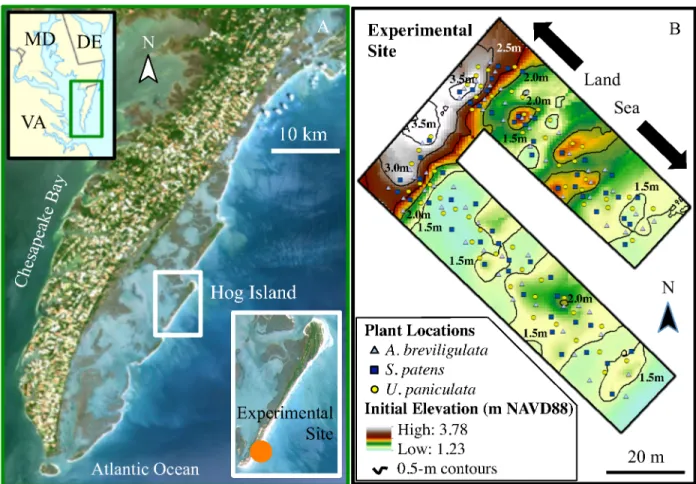
The Virginia Barrier Islands are located on the Eastern Shore of Virginia and comprise the southern stretch of the Delmarva Peninsula. The southern half of this island chain consists of twelve largely undeveloped, mixed-energy barrier islands (Hayes 1979), owned by The Nature Conservancy (TNC), and known as the Virginia Coast Reserve (VCR). Hog Island (located in the middle of the VCR—Figure 2A) is characterized by high topography and dominance of A. breviligulata and S. patens (Wolner et al. 2013; Dilustro and Day 1997).
The field portion of this study took place on the accretional (Fenster and Dolan 1994) southern end of Hog Island (Figure 2), which provides an ideal location to study A. breviligulata, U. paniculata, and S. patens not only because it is within the naturalized range of each species
2.2. Coastal Dune Model
What follows is a brief description of the coastal dune model developed by Durán and Moore (2013), which I will use to explore the effect of frontal-to-basal area on maximum dune height (see Durán and Moore (2013) for more detail). This model simulates the evolution of a sandy, vegetated surface (from the foreshore, across the backshore, and beyond the dune) by calculating aeolian transport and the resultant changes in sand-surface elevation (∂h/∂t) and vegetation cover fraction (∂ρveg/∂t) through time. All model simulations shown in this study were conducted under conditions of a stable foreshore (i.e., the shoreline does not accrete or erode), and a constant onshore wind speed (Table 1).
The coastal dune model captures the two-way interactions between vegetation and sand transport that give rise to coastal foredunes. As the initial model surface evolves, generic ‘plants’ are able to grow from an initial density of 0 when a given cell is beyond a minimum distance to the shoreline (Lveg; the vegetation limit). This generic species has a maximum cover fraction (ρveg) of 1 and maximum height (Hveg) of 1 m, and for simplification, reaches its maximum growth in 3 model days (tveg). Plant growth (∂ρveg/∂t) is modified by sand accretion (∂h/∂t) such that plant growth is maximized when sand accretion is zero, and growth decreases as sand accretion either increases or decreases. Additionally, as vegetation grows (∂ρveg/∂t) in a given cell, surface shear stress (τ) is reduced, leading to decreased aeolian sand transport capacity and a growth in the sand surface (∂h/∂t). The reducing effect of vegetation on wind shear is calculated with the wind shear reduction parameter Γ from Durán and Hermann (2006), based on the work of Raupach et al. (1993):
τs = τ
1+Γρmax
Γ= mβ
σ (1.2)
Where τs is the surface wind shear stress in a vegetated area, τ is the surface wind shear in an non-vegetated area, ρmax is the maximum plant cover fraction, β is the ratio of plant to surface drag coefficients, m is an empirical fitting parameter, and σ is the ratio of plant basal area to frontal area. The empirical parameter m takes into account the ratio between average and maximum wind shear stress at the surface across the entire area of interest (Wyatt and Nickling 1997). Durán and Moore (2013) parameterize (1.1) and (1.2) based on previous work on desert creosote shrubs. It is these parameterizations that will be replaced below with empirically derived measurements of plant basal and frontal area.
3. METHODS
3.1. Experimental setup
On May 21, 2014, I planted 2 individuals of each species at 30 locations in each of two ~25 m wide cross-shore swaths on the southern end of Hog Island (Figure 2B) (for a total of 360 plants at 180 locations). Using transplants that had been grown from seed in greenhouses, I first sorted seedlings by length and number of stems and then selected the intermediate-sized
To minimize the effect of plant mortality due to transplant shock on my results I replaced dead plants with live ones from the reserve garden (which was cared for in the same way as the experimental plantings) until June 23. Upon initial and replacement planting, I applied 300 mL of fresh water at the base of the plant. I applied an additional 120 mL of fresh water to each plant on May 21, 22, 23, and 29, and June 5, 9, 13, and 23. To reduce competition with pre-existing vegetation, I removed (monthly) the aboveground biomass of pre-existing vegetation within 1 meter of each plant location, measured from the fiberglass stake. On June 24, I removed the aboveground biomass of the plant with fewer or weaker leaves at each location to reduce competition between adjacent transplants. If the removed plant grew back, its aboveground biomass was removed monthly.
Based on data collected at a meteorological station on Hog Island (Porter et al. 2014a) the summer of 2014 was wetter than average (Figure 2A-B), and thus the transplants in this
experiment received more precipitation than would be expected in a normal summer in this location. Rainfall events delivering in excess of 20 cm of rain were more frequent in 2014, especially in July, than in the two years previous (Figure 3A), and precipitation in September was greater than 1 standard deviation higher than the September mean computed over the last 25 years (Figure 3C). Wind predominantly blew onshore over the field season, with dominant modes from the south and from the southeast (Figure 3C).
21 to October 14) (Figure 3A) and combined with an astronomical spring high tide on September 10 to generate one of the highest high water events observed throughout the field season.
Plant locations varied from 21.3 m to 103.5 m in distance to the shoreline, and from 1.25 to 3.78 m in initial elevation. The locations highest in elevation were on the foredune ridge, whereas those lowest in elevation were at the foredune toe and the seaward edge of transect A (the southernmost swath). To cover a wide gradient of distance to shoreline and elevation, I installed transplants across two protodunes located in the northern swath at approximately 50 to 70 m and 80 to 85 m from the shoreline, having maximum elevations of 2.4 and 2.5 m,
respectively, and on a single, smaller protodune (maximum elevation of 2.0 m) in the southern swath between 40 and 50 m from the shoreline (Figure 2B).
3.2. Measurements
I made a series of measurements and observations (longest leaf, plant state and elevation) monthly from June to October in 2014. I measured longest visible leaf length to the nearest millimeter with a repeatability of +/- 1 mm between observers, and this is the measurement used in allometric relationships. In cases where the sand surface at a plant location eroded, I measured the longest visible leaf from the base of the plant – not the sand surface around the transplant soil plug. I calculated longest leaf length—the measure of plant growth used in regression analyses— by subtracting the initial elevation from the October elevation at each plant site and then adding that value (if it was positive) to the measurement of longest visible leaf collected in the field to account for accretion at each plant site.
classified plants as “Healthy,” “Stressed,” “Dead,” or “Missing,” and I collected photographs of each plant for additional evidence of plant state (Figures S1-S3, Appendix 3).
To measure elevation, I installed two GPS monuments on the secondary dune ridge at the experimental site, collected the UTM coordinate and NAVD88 elevation of one using a Trimble R6, and post-processed the point using the National Geodetic Survey’s Online Positioning User Service (NGS-OPUS) (XY error = 0.008 m, Z error = 0.022 m). I then used a Nikon DTM-322 total station to measure the elevation of the second monument (angle error = 5 arcseconds), and confirmed its position with a later GPS survey according the procedure described above. I then used the total station and backsight to survey the elevation at the fiberglass stake at each plant location, as well as in the reserve garden. I also collected four monthly cross-shore beach profiles along repeated transect lines (one through each experimental swath, and one each to the north and the south of the two swaths) from the primary foredune to the water line by collecting a point at each change in slope along the profile (Figure 4). To measure distance to the shoreline, I calculated the NAVD88 elevation of mean high water (MHW) at the experimental site (0.46 m NAVD88) using VDATUM (NOAA). Using ArcGIS, I then created a shore-parallel line at this elevation in the June topographic survey and measured the shortest shore-perpendicular distance from that line to each plant location. I made additional measurements (lateral spreading, basal area, and frontal area) at the beginning and/or end of the field season. Similar to plant mortality, I measured lateral spreading visually as a binary variable (spreading vs. no spreading). Given that each species has a different growth habit and rate of lateral spreading I identified lateral
(Figure S4). To measure the basal and frontal area of each plant, I photographed each plant in the plan (basal) and front (frontal) view in June and October, then used the ImageJ software package to calculate the plant area in square centimeters (Figure S5).
I made two measurements on September 10 that were only possible due to the high water event on that day. First, I measured the salinity of a water sample from a pool of standing water near the foredune toe, and second, I surveyed the elevation of a wet/dry line on the foredune and protodunes, then calculated the average elevation of these points.
For more details on methods, please see Appendix 1. 3.3. Data Analysis
I created interpolated surfaces in ArcGIS based on the monthly elevation surveys, then used the Minus function in ArcGIS to subtract the June surface from the October surface. This created a topographic change map for the growing season (Figure 5).
I calculated total water level using data from a tide gauge on the north side of Hog Island (Porter et al. 2014b) and a wave buoy offshore of Cape Henry, VA (NOAA/Scripps Institution of Oceanography Waverider Buoy #44099, 36°54’55” N, 75°43’12” W). I then compared the TWL record to plant mortality (Figure 6A), calculated as a percentage: the number of missing or dead plants within a 0.1-m bin observed in a given month divided by the total number of plants present in the previous month.
The high water event of September 10 resulted in pools of standing water at low
elevations for at least one day. The tide was the highest of the field season on this day (Porter et al. 2014b), but the total water level (TWL, defined as the measured water elevation plus the elevation of runup of the highest 2% of waves, Ruggiero et al. 2001) at the experimental site was higher on October 4. But, since I was able to make measurements at the field site on September 10, to capture the impacts of a high water event on topography and plant growth, and to measure the salinity of surface water near the dune, I focus below on the event of September 10th.
measured at the end of the growing season in October by basal area, plant health, and lateral spreading across all species and all three elevation zones.
For these categorical plant growth and elevation analyses, I compared log basal area to elevation classes using 1-way ANOVA; and compared plant health and lateral spreading to elevation classes using a Chi-squared test. I performed a log transformation on basal area values before analysis to give the data a more normal distribution and enable the use of ANOVA instead of a less statistically powerful non-parametric test (e.g. Kruskal-Wallis) (Figure 10A inset).
Model runs in this study followed the parameterization of Durán and Moore (2013), with the addition of a Heaviside function in the vegetation dynamics equation describing a minimum elevation above mean sea level (MSL) for vegetation growth (zmin, Durán and Moore 2014) (Table 1). I varied the ratio of basal-to-frontal area (σ) across values ranging from 0.1 to 2.0, and varied the empirical fitting parameter m over the range 0.1 to 0.2, incorporating the values suggested by Wyatt and Nickling (1997).
4. RESULTS
4.1. Topographic change
temporarily lowered the topography by 0.2 m at a distance of approximately 150 m from the June shoreline along this transect.
4.2. Growth relationships
In the 2014 growing season, A. breviligulata transplants grew to a maximum longest leaf length of 928 mm and maximum basal area of 2402 cm2. For S. patens, these values were 792 mm and 1018 cm2, and for U. paniculata, they were 1185 mm and 2869 cm2.
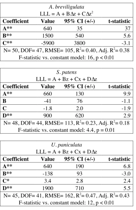
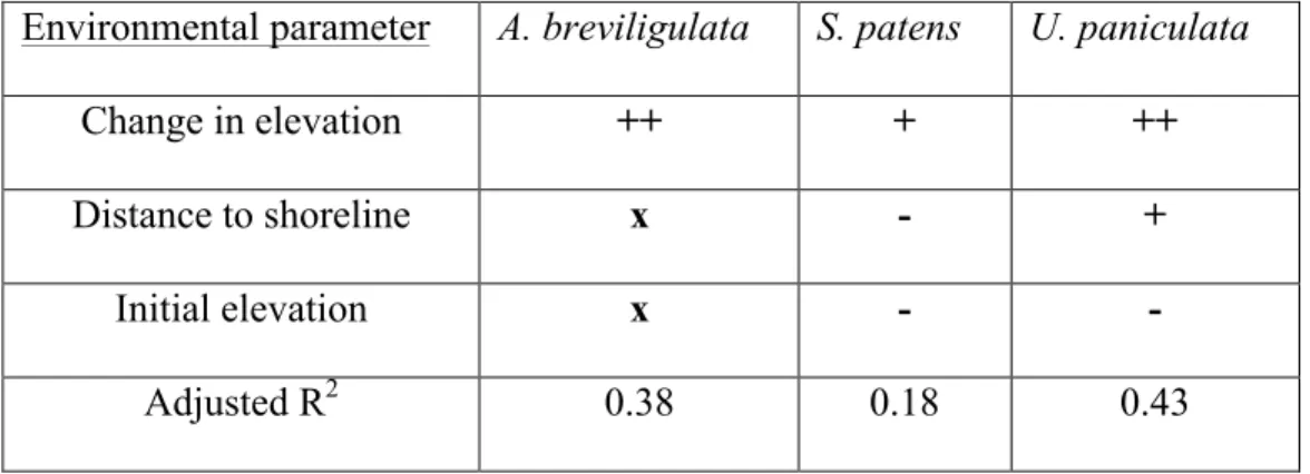
In A. breviligulata, longest leaf length was significantly correlated with change in elevation through a quadratic equation, and in S. patens and U. paniculata, longest leaf length was significantly correlated with all three environmental parameters (distance to shoreline, initial elevation, and change in elevation) through a multiparameter linear equation (Tables 2 and S1; p<0.01, p=0.01, p<0.01; Adjusted R2=0.38, 0.18, 0.43; respectively). In A. breviligulata, longest leaf tended to increase with change in elevation up to 0.13 +0.35/-0.08 m of change, after which longest leaf tended to decrease (Figure 8D). Increases in change in elevation and decreases in distance to shoreline and initial elevation were correlated with increases in longest leaf length in S. patens (Table 2), and these relationships held at a higher level of significance but equal level
of predictive power when distance to shoreline and initial elevation were analyzed separately from one another (Table S1, Appendix 2). In U. paniculata, increases in distance to shoreline and change in elevation and decreases in initial elevation were significantly correlated with longest leaf length (Table 2).
Tables S2-S4). Longest leaf length had a significant, positive, simple linear correlation with change in elevation in A. breviligulata and in U. paniculata, but not in S. patens (Figure 8A-C; p<0.01, p=0.11, p<0.01; R2=0.28, 0.05, 0.34; respectively). Quadratic regression yielded a significant relationship between longest leaf length and change in elevation in A. breviligulata only (Figure 8D-F).
Large differences in the magnitudes of the coefficients in these relationships arise from differences in the ranges of each environmental parameter (~20–120 m for distance to shore; ~1– 4 m for initial elevation; ~ -0.2 – +0.3 m for change in elevation), and when these coefficients are rescaled to units on the same order of magnitude, regression results (p, t, F statistics) do not change. Belsley’s test for collinearity returned collinearity indices less than 11 for all
combinations of independent variables in all species – far lower than the threshold level of 30 – indicating that multicollinearity did not significantly affect my results. Additionally, sample size was large enough (N>>15) for all relationships to be robust to modest violations of normality, though probability plots of residuals showed no such violations.
Plant mortality qualitatively tended to be observed after high water events (Figure 6A) and at the edges of swaths, dunes, and protodunes (Figure 6B).
4.3. Plant Growth and Access to Water
~1.5 m and ~1.75 m. Nonlinear regression on the basal area vs. initial elevation data produces a fitted power-law equation (RMSE=387, lower for A. breviligulata and S. patens), and
qualitatively shows the nature of the relationship between basal area and initial elevation (Figures 9A, S7). These power-law equations are descriptive of my data and should not be interpreted as describing a physical process due to the large exponential terms (~x8).
The salinity of the standing water near the foredune toe on September 10th was 0.15 ppt, indicating a freshwater source. Living plants in the low zone had significantly larger
log-transformed basal areas than those in the mid zone or high zone. (340 vs. 95 and 107 cm2,
respectively, 1-way ANOVA, p<0.01) (Figure 10A). A Kruskal-Wallis test on the untransformed data yielded qualitatively the same result as the ANOVA test on the log-transformed data, and p-values for both were orders of magnitude lower than 0.01. These relationships hold when
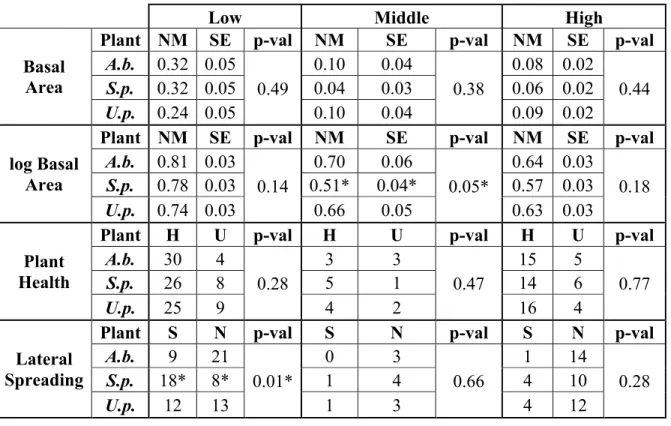
normalizing each individual measurement by dividing the longest leaf lengths and basal areas of each plant by the maximum of each species. Plants were not significantly healthier in any zone compared to the others (Chi-square, p=0.47; Figure 10B), but healthy plants in the low zone were significantly more likely to spread laterally than those in the mid or high zones (Chi-square, p<0.01; Figure 10C).
4.4. Plant Basal vs. Frontal Area
My field data provides quantitative constraints on the ratio of basal-to-frontal area (σ, Durán and Hermann 2006, Durán et al. 2008, Durán and Moore 2013) most appropriate for dune-building grasses. All dune grasses in this experiment had σ = 0.8 +/- 0.3 (mean +/- 1 S.D.), which differs significantly from the mean value of ~1.5 reported for creosote bushes (Wyatt and Nickling 1997) and Brazilian dune plants (Durán et al. 2008) (Figure 11A).
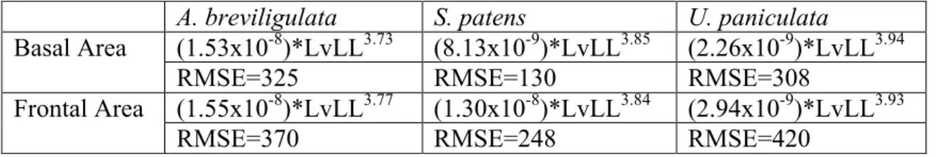
Basal and frontal area measurements are difficult and time-consuming to make, both in the field and in post-processing. However, longest visible leaf measurements are simple, quick, and require no post-processing. For this reason, I investigated the relationship between longest leaf length and plant size, and I derived allometric relationships for basal and frontal area as a function of longest visible leaf length, which take the form y=Axb (where y is the basal or frontal area, x is the longest visible leaf length, and A and b are coefficients)(Figure 12, Table 4).
In the coastal dune model of Durán and Moore (2013), an increase in the ratio of basal to frontal area acts to amplify the reducing effect of vegetation on surface wind shear and thereby reduce the wind shear near a plant (Equations 1 and 2). Results from this model showed that changes in the ratio of basal area to frontal area had a nonlinear effect on maximum dune height (Figure 11B). As the ratio increased (greater basal area proportional to frontal area), dune height increased until the ratio reached ~0.85, then decreases sharply when the ratio is equal to 1.3. At ratios greater than 1.3, dune height tended to decrease gradually. This nonlinearity arose from the mathematical relationship between wind shear stress and vegetation (Equations 1 and 2). The ratio of basal-to-frontal areas did not vary significantly among the species in this study; therefore modeled maximum dune height in my experiment was not controlled by species-specific
Varying the empirical fitting parameter m changes the BA/FA value at which the nonlinear transition occurs (Figures 11, S8). Within the range suggested by Wyatt and Nickling (1997), m has a small effect on maximum dune height, but the effect of m increases as the ratio of basal-to-frontal area increases. The m parameter also acts to change the BA/FA value at which the nonlinear transition occurs- when m equals 0.1, the nonlinear transition in dune height occurs around a BA/FA value of 0.9 (instead of 1.3), and an increase in m by 0.02 units causes the center of the nonlinearity to increase by 0.2 BA/FA units.
5. DISCUSSION
5.1. Growth relationships
Multiparameter regression suggests significant species-specific correlations between growth (as measured by longest leaf length) and distance to shoreline, elevation, and change in elevation that were not apparent from simple regression analyses (Table 2, Figure S6). For A. breviligulata and U. paniculata, these environmental parameters accounted for a fairly large
portion of the variance in growth among individuals (Adj. R2= 0.38 and 0.43 respectively), but these parameters were not as strong of a predictor of growth in S. patens (Adj. R2=0.18). The ability of S. patens to occupy a wider range of environments (Anderson and Alexander 1985; Craig 1975; Stalter et al. 1999) than A. breviligulata or U. paniculata may explain the relative lack of predictive strength in the correlation between the longest leaf length of S. patens and environmental conditions across the dune and beach.
For A. breviligulata, change in elevation was the only environmental parameter
in elevation was taken into account, longest leaf length was significantly positively correlated with change in elevation and negatively correlated with initial elevation and distance to the shoreline (Tables 2 and S1). When change in elevation, distance to the shoreline, and initial elevation were considered together, only change in elevation was significantly correlated with longest leaf length (Table 2). When considering each parameter individually for U. paniculata, longest leaf length was significantly positively correlated only with change in elevation (Figure 8). However, when all factors were considered together, longest leaf length was significantly positively correlated with distance to the shoreline and change in elevation, and significantly negatively correlated with initial elevation (Table 2). These results are summarized in Table 5.
The tendency for salt spray and soil salinity to decrease with increasing distance from the shoreline and the increased ability of S. patens over U. paniculata to cope with salinity stress (Seneca 1972) may account for the difference in sign of the correlation for these two species. The negative correlation between longest leaf length and initial elevation (i.e., faster growth at low elevations) observed in both species may be due to increased availability of water at low elevations (Section 5.2).
sand accretion and plant growth across species. That plant growth and change in elevation are positively correlated (i.e., faster growth is associated with accretion/burial) for individuals of U. paniculata provides quantitative evidence in further support of its classification as an effective
“dune-builder” (e.g., Woodhouse 1982; Ehrenfeld 1990; Stallins 2002; Stallins 2005), and the same is true for A. breviligulata up the rate of change in elevation that maximizes plant growth (i.e., 0.13 +0.35/-0.08 m over 5 months). Additionally, the less positive correlation in S. patens between the same two factors agrees with literature (Travis 1977; Stallins 2005; Wolner et al. 2013; Brantley et al. 2014) characterizing S. patens as a grass tolerant of, but not as responsive to, sand accretion as other dune-building species. The quadratic relationship I derived for A. breviligulata is similar to that derived by Maun and Perumal (1999) relating sand burial to cover
of A. breviligulata. When the data points with the four most extreme ∆z values were removed from the A. breviligulata data, the quadratic equation no longer significantly fit the data, but change in elevation was still the only environmental factor significantly correlated with longest leaf length (Table S5).
Continuing work with this dataset and data from the same plants over a second growing season will further investigate the relationship between sand accretion, plant growth, and
multiplier could be set to unity, as growth in A. breviligulata was not significantly correlated with distance to the shoreline.
Though plant growth was significantly correlated with distance to shoreline, initial elevation, and change in elevation, controls on mortality and the associated cross-shore vegetation limit (i.e., Lveg, Durán and Moore 2013) were not apparent in data arising from the first growing season of this field experiment (Figure 6B). If the seaward limit beyond which dune-building vegetation does not successfully grow arises from plant responses to stresses associated with beach position (e.g., salt spray, sand burial, wind, etc.), it may be that it will take longer than one growing season for these stresses to cause mortality in my transplants.
Alternatively, if this limit is controlled by responses to physical processes associated with storms—such as high total water levels and an elevated zone of wave action—it is possible that the plants in my experiment, which were artificially planted near the shoreline as fairly
vegetation establishing seaward of the dune crest up to the extreme limit of runup, further suggesting a link between TWL and vegetation zonation.
Additionally, it is possible that individual plant survival during storms depends on plants becoming established, accreting sand, and potentially binding this sand with their roots against wave action (as occurs in fluvial and riparian systems (e.g., Gurnell et al. 2001, Tabacchi et al. 2000) between high water events. In my experiment, two plants (marked in Figure 6B) were established and growing before they were killed and removed during HWEs. The older, denser preexisting vegetation at similar distances from shoreline and elevations, which presumably had a larger, denser root system than did the transplants, survived the same high water events. It is possible that with the increased stabilization afforded by large root systems, these plants would have survived the high water events had they occurred after the plant had become more
established.
Decreased survival along the edges of swaths and protodunes, along with qualitatively high rates of growth and topographic change in the reserve garden (personal observations), points to a potential facilitative relationship among dune grass individuals (which we are preparing to explore in future experiments) promoting growth, survival, and density, as
suggested by Castanho and colleagues (2015). This idea is in agreement with the Stress Gradient Hypothesis (e.g. Bertness and Callaway 1994; He et al. 2013), which predicts that high levels of stress will lead to increased facilitative relationships among individuals.
5.2. Plant Growth and Presence of Water
Longest leaf length and initial elevation had a significant negative correlation in S. patens and U. paniculata (Tables 2 and S1), and in general, transplants of all species installed at low elevations had larger basal areas and were more likely to spread than those at higher elevations (p<0.01, Figure 10).
Due to the observed patterns of plant growth, I believe that in addition to change in elevation, access to water is important in determining plant growth, especially for transplants, which have shallow root systems and therefore cannot access groundwater when planted at higher elevations. The low salinity in the water sample collected from the isolated pool of surface water on the backshore following the coincident rain event of September 7-9 and the HWE of September 10, suggests that in low areas following rainstorms and/or HWEs, accumulations of fresh water and/or groundwater pumped upward from the freshwater lens during the tidal cycle may provide access to water for plants at low elevations, potentially allowing them to grow more than the transplants at higher elevations. Though this appears to conflict with previous findings in U. paniculata (Oosting and Billings 1942; Hester and
1987), none of these studies investigated plant growth along a continuum of elevation in the field. Future work will investigate the elevation and salinity of the water table at the
experimental site and provide more insight into the groundwater hypothesis.
It follows that transplants installed at relatively high elevations (as they are in dune restoration projects) would benefit from having long root systems at the time of installation so that they are able to reach the groundwater table as consistently as transplants installed at relatively lower elevations, or from being installed at a lower initial elevation (consistent with Nordstrom et al. 2000, Nordstrom 2008). In naturally evolving systems, such elevation-related sensitivity to water is likely diminished because grasses grow upward as the sand surface accretes (e.g. Ehrenfeld 1990, Gilbert and Ripley 2010), leading to the development of deep roots which extend deep into the subsurface, likely to the base of the dune.
5.3. Plant Basal and Frontal Area
The ratio of basal-to-frontal area of the transplants in my field experiment is close to the value that maximizes dune height in the coastal dune model of Durán and Moore (2013) when the m parameter is equal to 0.16 (as in Durán and Moore 2013; 2014). Several studies correlate dune morphology to vegetation morphology (Hesp 2002, Hacker et al. 2011, Zarnetske et al. 2012, Seabloom et al. 2013) and model results presented here—which show that the ratio of plant basal-to-frontal area exerts a nonlinear control on maximum dune height—suggest that the model is capturing this dependence. All other factors being equal (e.g., sand supply, wind direction and velocity, tidal range, etc.), dunes built by the grass species of interest in this experiment (A. breviligulata, S. patens, U. paniculata) and other grasses of similar shape (BA/FA = 0.8) will be taller than those built by grasses of a shape more similar to those
This suggests that measuring the basal and frontal area for different dune grass species may be important in predicting the maximum dune height that can naturally be achieved in a given location and the protection from overwash and inundation that may be afforded by dunes built by different grass species.
It is possible that the lower ratios of basal-to-frontal area observed in my experiment were due to individual transplants being installed with ample space to spread out in the lateral dimensions to absorb light. In a naturally spreading dune system in which plants are spreading clonally, individual plants are packed densely together, and plants are thereby forced to grow more vertically than horizontally to absorb light, and this could have lead to an artificially decreased ratio of basal-to-frontal area in my experiment (future experiments will compare the ratios of basal-to-frontal area of transplants to plants naturally growing in the experimental site).
Since basal and frontal area are important parameters controlling dune height, it is useful that longest visible leaf length predicts basal and frontal area through an allometric scaling relationship for each species (Table 4). Basal and frontal area are difficult and time-consuming measurements, both in the field collection stage and in the image processing stage, but longest visible leaf length is a very simple and quick field measurement that requires no further processing.
6. CONCLUSIONS
Transplant longest leaf length was most significantly correlated with change in elevation in all species, and growth was also correlated with distance to shoreline and initial elevation in S. patens and U. paniculata. Quadratic regression suggested a maximum in plant growth of A.
breviligulata at an accretion rate of ~0.1 m over one growing season. Distance to shoreline was
(positive), possibly due to differences in salinity tolerance in each species. Longest leaf length and initial elevation had a significant negative correlation in S. patens and U. paniculata, and transplants of all species were largest and most likely to spread at low elevations, and I attribute this to increased access to water. Future modeling work will investigate species-specific effects on foredune morphology in response to environmental parameters.
Additionally, longest visible leaf length scales allometrically with basal and frontal area across species, enabling the use of a simple measurement to approximate aerodynamic roughness parameters. Though the ratios of basal to frontal area are different for the U.S. East coast dune grasses (0.8) than for plants studied previously (1.5), they do not vary significantly among the East coast species, and this ratio exerts a nonlinear control on maximum foredune height predicted by the Durán and Moore (2013) coastal dune model. Simulations suggest that, other factors being equal, foredunes are highest at a ratio of basal-to-frontal area of ~0.8, which is the ratio measured for the East coast dune-building grasses.
From my results, I extrapolate that restoration projects working to optimize
TABLES
Parameter
Name Description
Value
Used Reference
NX Cross-shore
cells 100 Durán and Moore (2013)
NY
Shore-parallel cells 4 Durán and Moore (2013)
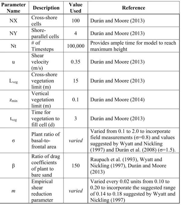
Nt # of Timesteps 100,000 Provides ample time for model to reach maximum height
u
Shear velocity (m/s)
0.35 Durán and Moore (2013)
Lveg
Cross-shore vegetation limit (m)
15 Durán and Moore (2013)
zmin
Vertical vegetation limit (m)
0.1 Durán and Moore (2014)
tveg
Time for vegetation to
fill cell (d) 3 Durán and Moore (2013)
σ
Plant ratio of
basal-to-frontal area varied
Varied from 0.1 to 2.0 to incorporate field measurements (σ=0.8) and values suggested by Wyatt and Nickling (1997) and Durán et al. (2008) (σ=1.5).
β
Ratio of drag coefficients of plant to bare sand
150 Raupach et al. (1993), Wyatt and Nickling (1997), Durán and Moore (2013) m Empirical shear reduction parameter varied
Varied every 0.02 units from 0.10 to 0.20 to incorporate the suggested range of 0.14 to 0.18 suggested by Wyatt and Nickling (1997)
Table 1. Parameter list. List of parameters used in the modeling portion of this experiment and
A. breviligulata
LLL = A + B∆z + C∆z2
Coefficient Value 95% CI (+/-) t-statistic
A** 640 35 37
B** 1500 540 5.6
C** -5900 3800 -3.1
N= 50, DOF= 47, RMSE= 105, R2
= 0.40, Adj. R2
= 0.38 F-statistic vs. constant model: 16, p < 0.01
S. patens
LLL = A + Bz + Cx + D∆z
Coefficient Value 95% CI (+/-) t-statistic
A** 660 130 9.9
B -41 76 -1.1
C -1.8 2.0 -1.9
D** 900 620 2.9
N= 48, DOF= 44, RMSE= 113, R2
= 0.23, Adj. R2
= 0.18 F-statistic vs. constant model: 4.4, p = 0.01
U. paniculata
LLL = A + Bz + Cx + D∆z
Coefficient Value 95% CI (+/-) t-statistic
A** 640 190 6.8
B** -138 93 -3.0
C* 3.4 2.8 2.4
D** 1900 710 5.5
N= 45, DOF= 41, RMSE= 162, R2
= 0.47, Adj. R2
= 0.43 F-statistic vs. constant model: 12, p < 0.01
Table 2. Results of multiparameter regression. Optimized multiparameter equations (based on
combination of significant coefficients and adjusted R2 values) relating longest leaf length (mm) to distance to shoreline, initial elevation, and change in elevation (m) in each species.
Coefficients, 95% confidence intervals, and the t-statistic for each variable are shown, with p values <0.05 marked with * and p values <0.01 marked with **. Goodness-of-fit statistics (Number of replicates (N), Degrees of freedom (DOF), Root mean square error (RMSE), R2,
Low Middle High
Basal Area
Plant NM SE p-val NM SE p-val NM SE p-val A.b. 0.32 0.05
0.49
0.10 0.04
0.38
0.08 0.02
0.44 S.p. 0.32 0.05 0.04 0.03 0.06 0.02
U.p. 0.24 0.05 0.10 0.04 0.09 0.02
log Basal Area
Plant NM SE p-val NM SE p-val NM SE p-val A.b. 0.81 0.03
0.14
0.70 0.06
0.05*
0.64 0.03
0.18 S.p. 0.78 0.03 0.51* 0.04* 0.57 0.03
U.p. 0.74 0.03 0.66 0.05 0.63 0.03
Plant Health
Plant H U p-val H U p-val H U p-val
A.b. 30 4
0.28
3 3
0.47
15 5
0.77
S.p. 26 8 5 1 14 6
U.p. 25 9 4 2 16 4
Lateral Spreading
Plant S N p-val S N p-val S N p-val
A.b. 9 21
0.01*
0 3
0.66
1 14
0.28
S.p. 18* 8* 1 4 4 10
U.p. 12 13 1 3 4 12
Table 3. Species comparison within elevation zones. Comparisons among species within three
A. breviligulata S. patens U. paniculata
Basal Area (1.53x10⁻⁸)*LvLL3.73 (8.13x10⁻⁹)*LvLL3.85 (2.26x10⁻⁹)*LvLL3.94
RMSE=325 RMSE=130 RMSE=308
Frontal Area (1.55x10⁻⁸)*LvLL3.77 (1.30x10⁻⁸)*LvLL3.84 (2.94x10⁻⁹)*LvLL3.93
RMSE=370 RMSE=248 RMSE=420
Table 4. Longest visible leaf length vs. Basal and Frontal Areas. Allometric relationships
Environmental parameter A. breviligulata S. patens U. paniculata
Change in elevation ++ + ++
Distance to shoreline x - +
Initial elevation x - -
Adjusted R2 0.38 0.18 0.43
Table 5. Summary of multiparameter regression. Summary of the results of multiparameter
FIGURES
Figure 1. Species of interest in this experiment. Ammophila breviligulata (A), Spartina patens
Figure 2. Experimental site maps. Location of experimental site on Hog Island in larger
geographic area (A, NASA Thematic Mapper LANDSAT 7 Thematic Mapper Scene of Virginia Portion of the Delmarva Peninsula – 1999, data available at www.usgs.gov and
Figure 3. Hog Island 2014 weather. Daily (A) and monthly (B) precipitation, along with
Figure 4. Monthly cross-shore beach profiles. Cross-shore beach profiles surveyed monthly
Figure 5. Topographic change within experimental site. Change in elevation in the
Figure 6. Plant mortality. A. Plant mortality vs. Total water level. Percentage of missing or
dead plants compared to the total number of plants in previous month. Missing or dead plants are shown at the elevation and date on which they were first observed to be missing or dead, and then are removed from future calculations. Total Water Level (calculated as in Ruggiero et al. 2001) at Hog Island over 2014 experimental season calculated from tide gauge on Hog Island is overlain in blue, with tide gauge error in black dashes. B. Cumulative plant mortality across experimental site as of October 2014. Note high mortality along the edge of each swath and at the edge of protodunes, as well as locations of plants removed in HWEs (mentioned in
Figure 7. Elevation classification map. Plant locations in each elevation classification zone
Figure 8. Longest leaf length vs. change in elevation. Transplant longest leaf length (mm) in
A. breviligulata (A, D), S. patens (B, E), and U. paniculata (C, F) as a function of change in
Figure 9. Basal area vs. Initial elevation. A. Nonlinear relationship between basal area and
Figure 10. Categorical plant growth comparisons. Plant Log basal area (A, p<0.01), Health
(B, p=0.47), and Spreading (C, p<0.01) across species in each elevation classification based on maximum total water level for growing season. Panel A: Red line= mean, red shade= 95% CI, black dots= data points. Histograms in panel A inset show untransformed basal area and log-transformed basal area. Plot in A generated using Matlab Central File Exchange file
Figure 11. Measurement and modeling of ratio of frontal area. A. Ratio of
Figure 12. Allometric relationships between longest visible leaf length, basal area, and
frontal area. Allometric relationships between longest visible leaf length (LVLL, [mm]) and
APPENDIX 1: SUPPLEMENTARY METHODS
1.1 Experimental setup
I coded each plant according to its location. For example, the plant labeled “SB16L” is the leftward plant as one faces the dune (southernmost plant) at the 16th S. patens site from the shoreline on the northern swath, while the plant labeled “UA3R” is the rightward plant as one faces the dune (northernmost plant) at the 3rd U. paniculata site from the shoreline on the southern swath.
Two noteworthy meteorological events occurred at my experimental site during the 2014 growing season. First, the eye of Hurricane Arthur passed approximately 150 km to the south of my experimental site on July 4, 2014, bringing winds of 11.5 m/s to Hog Island (Porter et al. 2014a), 90 mph at the eye wall, and 45 mph at the NOAA Wallops Island Station, 65 km north of my experimental site. Second, an intense rainfall event over September 7-9 (138.38 mm of rain over the 3 days, Porter et al. 2014a) and an astronomical spring high tide combined to generate one of the highest high water events observed throughout the field season in my experimental site. Rainfall on September 9, 2014, at the NOAA meteorological station in nearby Norfolk, VA, recorded the highest 24-hour rainfall total on record (NOAA online data
http://www.erh.noaa.gov/er/akq/climate/ORF_Climate_Records.pdf)
respectively. Additionally, there was a single, smaller protodune on transect A (maximum elevation of 2.0 m) between 40 and 50 m from the shoreline (Figure 1B).
1.2 Measurements
I made a series of measurements and observations (longest leaf, plant state and elevation) monthly from June to October in 2014. To measure longest leaf length, I collected all the leaves of the plant, raised my hands to allow the shortest leaves to fall out, and then grasped the last leaf remaining. I placed a meter stick with an attached metal 90-degree joint on the sand surface and touching the base of the longest leaf, then recorded leaf length to the nearest millimeter. One lab member measured plants while another recorded the data. I measured plant mortality, or “plant state,” by visually observing the color, uprightness, and number of each plant’s leaves, as well as the presence or absence of each plant. Plants were then classified as “Healthy,” “Stressed,” “Dead,” or “Missing,” and I collected photographs of each plant for additional evidence of plant state (Figures S1-S3).
southern swath (“TS”) (Figure 5). Beach profiles started at the primary foredune crest and terminated at the water line; for this reason, each profile does not end at the same distance from the dune.
Salinity of the water sample was measured in the lab with a Hanna Instruments 98130 pH/conductivity/salinity/Total Dissolved Solids meter.
APPENDIX 2: SUPPLEMENTARY TABLES
S. patens
LLL = A + Bz + C∆z
Coefficient Value 95% CI (+/-) t-statistic
A** 600 120 9.9
B* -80 65 -2.5
C* 830 630 2.7
N= 48, DOF= 45, RMSE= 116, R2
= 0.17, Adj. R2
= 0.13 F-statistic vs. constant model: 4.6, p = 0.01
LLL = A + Bx + C∆z
Coefficient Value 95% CI (+/-) t-statistic
A** 620 120 11
B** -2.4 1.6 -3.0
C* 800 580.0 2.7
N= 48, DOF= 45, RMSE= 113, R2
= 0.21, Adj. R2
= 0.18 F-statistic vs. constant model: 6.0, p < 0.01
LLL = A + Bz + Cx + D∆z
Coefficient Value 95% CI (+/-) t-statistic
A** 660 130 9.9
B -41 76 -1.1
C -1.8 2.0 -1.9
D** 900 620 2.9
N= 48, DOF= 44, RMSE= 113, R2
= 0.23, Adj. R2
= 0.18 F-statistic vs. constant model: 4.4, p = 0.01
Table S1. Multiple linear regression with S. patens. Comparison among three possible fit
LLL = A + Bz + Cx
A. breviligulata
Coefficient Value 95% CI (+/-) t-statistic
A** 670 140 9.4
B 12 74 0.3
C -0.6 2.3 -0.5
N= 50, DOF= 47, RMSE= 136, R2= 0.01, Adj. R2<0.01
F-statistic vs. constant model: 0.1, p = 0.88
S. patens
Coefficient Value 95% CI (+/-) t-statistic
A** 590 130 8.8
B -7.8 8.8 -0.2
C -1.4 2.1 -1.4
N= 48, DOF= 45, RMSE= 122, R2
= 0.08, Adj. R2
= 0.04 F-statistic vs. constant model: 1.9, p = 0.16
U. paniculata
Coefficient Value 95% CI (+/-) t-statistic
A** 590 240 4.9
B -70 120 -1.2
C 3.3 3.7 1.8
N= 45, DOF= 42, RMSE= 211, R2= 0.07, Adj. R2
= 0.03 F-statistic vs. constant model: 1.7, p = 0.20
Table S2. Multiple linear regression with distance to shoreline and initial elevation only.
LLL = A + Bz + Cx + D∆z A. breviligulata
Coefficient Value 95% CI (+/-) t-statistic
A** 720 120 12
B -23 64 -0.7
C -0.8 1.9 -0.9
D** 1200 540 4.6
N= 50, DOF= 46, RMSE= 114, R2
= 0.32, Adj. R2
= 0.27 F-statistic vs. constant model: 7.2, p < 0.01
S. patens
Coefficient Value 95% CI (+/-) t-statistic
A** 660 130 9.9
B -41 76 -1.1
C -1.8 2.0 -1.9
D** 900 620 2.9
N= 48, DOF= 44, RMSE= 113, R2
= 0.23, Adj. R2
= 0.18 F-statistic vs. constant model: 4.4, p = 0.01
U. paniculata
Coefficient Value 95% CI (+/-) t-statistic
A** 640 190 6.8
B** -138 93 -3.0
C* 3.4 2.8 2.4
D** 1900 710 5.5
N= 45, DOF= 41, RMSE= 162, R2= 0.47, Adj. R2
= 0.43 F-statistic vs. constant model: 12, p < 0.01
Table S3. Multiple linear regression with all environmental parameters. Possible fit
LLL = A + Bz + Cx + D∆z + E∆z2
A. breviligulata
Coefficient Value 95% CI (+/-) t-statistic
A** 720 110 13
B -4.6 60 -0.2
C -1.1 1.7 -1.2
D** 1600 560 5.8
E** -5800 3800 -3.1
N= 50, DOF= 45, RMSE= 105, R2
= 0.44, Adj. R2
= 0.39 F-statistic vs. constant model: 8.7, p < 0.01
S. patens
Coefficient Value 95% CI (+/-) t-statistic
A** 660 140 9.9
B -49 79 -1.2
C -1.8 2.0 -1.8
D 720 800 1.8
E 2600 7200 0.7
N= 48, DOF= 43, RMSE= 114, R2
= 0.24, Adj. R2
= 0.17 F-statistic vs. constant model: 3.4, p = 0.02
U. paniculata
Coefficient Value 95% CI (+/-) t-statistic
A** 660 190 6.8
B* -130 94 -2.8
C* 3.1 3.0 2.1
D** 2300 1100 4.1
E -3000 7000 -0.9
N= 45, DOF= 40, RMSE= 162, R2= 0.48, Adj. R2
= 0.42 F-statistic vs. constant model: 9.0, p < 0.01
Table S4. Multiple linear regression with all environmental parameters and quadratic
change in elevation. Possible fit equations relating longest leaf length (mm) to environmental
A. breviligulata
LLL = A + Bz + Cx + D∆z + E∆z2
Coefficient Value 95% CI (+/-) t-statistic
A** 750 110 14
B -18 63 -0.6
C -1.3 1.6 -1.6
D** 2500 1000 4.8
E -9600 15000 -1.2
N= 46, DOF= 41, RMSE= 96, R2= 0.47, Adj. R2= 0.42
F-statistic vs. constant model: 9.1, p < 0.01
LLL = A + B∆z
Coefficient Value 95% CI (+/-) t-statistic
A** 620 33 36
B 1700 690 4.8
N= 48, DOF= 43, RMSE= 114, R2
= 0.24, Adj. R2
= 0.17 F-statistic vs. constant model: 3.4, p = 0.02
Table S5. Multiple linear regression with A. breviligulata and large ∆z values removed.
APPENDIX 3: SUPPLEMENTARY FIGURES
Figure S1. Plant mortality in A. breviligulata. A. breviligulata transplants classified as Healthy
Figure S2. Plant mortality in S. patens. S. patens transplants classified as Healthy (A, plant
Figure S3. Plant mortality in U. paniculata. U. paniculata transplants classified as Healthy (A,
Figure S4. Lateral spreading in each species. Lateral spreading in A. breviligulata (A, plant
Figure S5. Basal and frontal area measurements. Steps in frontal area measurement of plant
Figure S6. Longest leaf length vs. initial elevation and distance to shoreline. Transplant
Figure S7. Basal area vs. initial elevation with power-law equations. Basal area vs. initial
Figure S8. Maximum dune height as function of basal-to-frontal area and m parameter.
REFERENCES
Anderson, L.C. and Alexander, L.L. 1985. The vegetation of Dog Island Florida. Florida Scientist 48 (4): 232-251.
Arens, S.M., Baas, A.C.W., van Boxel, J.H., and Kalkman, C. 2001. Influence of reed stem density on foredune development. Earth Surface Processes and Landforms 26: 1161-1176.
Barbier, E.B. et al. 2011. The value of estuarine and coastal ecosystems. Ecological Monographs 81: 169-193.
Barbour, M.G. and De Jong, T.M. 1977. Response of west coast beach taxa to salt spray, seawater inundation, and soil salinity. Bulletin of the Torrey Botanical Club 104: 29-34. Bertness, M.D. and Callaway, R. 1994. Positive interactions in communities. Trends in Ecology
and Evolution 9: 191-193.
Bindoff, N.L., Willebrand, J., Artale, V., Cazenave, A., Gregory, J., Gulev, S. et al. 2007. Observations: Oceanic Climate Change and Sea Level. In Solomon, S., Qin, D., Manning, M., Chen, Z., Marquis, M., Averyt, K.B. et al. (eds.): Climate Change 2007: The Physical Science Basis. Contribution of Working Group I to the Fourth Assessment Report of the Intergovernmental Panel on Climate Change. Cambridge University Press, Cambridge, United Kingdom and New York, NY, USA.
Brantley, S.T., Bissett, S.N., Young, D.R., Wolner, C.W.V., and Moore, L.J. 2014. Barrier island morphology and sediment characteristics affect the recovery of dune building grasses following storm-induced overwash. PLOS ONE. doi: 10.1371/journal.pone.0104747. Borsje, B.W., van Wesenbeck, B.K., Dekker, F., Paalvast, P., Bouma, T.J., van Katwijk, M.M. et
al. 2011. How ecological engineering can serve in coastal protection. Ecological Engineering 37 (2): 113-122.
Burdick, D.M. 1989. Root aerenchyma development in Spartina patens in response to flooding. American Journal of Botany 75 (5): 777-780.
Burdick, D.M. and Mendelssohn, I.A. 1987. Waterlogging responses in dune, swale and marsh populations of Spartina patens under field conditions. Oecologia 75 (3): 321-329. Castanho, C.d.T., Lortie, C.J., Zaitchik, B., and Prado, P.I. 2015. A meta-analysis of plant
facilitation in coastal dune systems: responses, regions, and research gaps. PeerJ 3:e768. doi: 10.7717/peerj.768.
Craig, R.M. 1975. Natural vegetation of Florida’s coastal dunes. Proceedings of the Soil and Crop Society of Florida 34: 169-171.
Crossett, K., Culliton, T.J., Wiley, P., and Goodspeed, T.R. 2004. Population trends along the coastal United States, 1980-2008. Silver Spring, MD: National Oceanic and Atmospheric Administration.
Crowell, M., Edelman, S., Coulton, K., and McAfee, S. 2007. How many people live in coastal areas? Journal of Coastal Research 23 (5): iii-vi.
de Winter, R.C., Gongriep, F., and Ruessink, B.G.. 2015. Observations and modeling of alongshore variability in dune erosion at Egmond aan Zee, the Netherlands. Coastal Engineering. ISSN 0378-3839, http://dx.doi.org/10.1016/j.coastaleng.2015.02.005. Dilustro, J.J. and Day, F.P. 1997. Aboveground biomass and net primary production along a
Virginia barrier island dune chronosequence. American Midland Naturalist 137 (1): 27-38.
Durán, O. and Moore, L.J. 2013. Vegetation controls on the maximum size of coastal dunes. Proceedings of the National Academy of Sciences of the United States of America 110 (43): 17212-17222. doi: 10.1073/pnas.1307580110.
Durán, O. and Moore, L.J. 2015. Barrier island bistability induced by biophysical interactions. Nature Climate Change 5: 158-162. doi: 10.1038/nclimate2474.
Durán, O., Silva, M.V.N., Bezerra, L.J.C., Herrmann, H.J., and Maia, L.P. 2008. Measurements and numerical simulations of the degree of activity and vegetation cover on parabolic dunes in north-eastern Brazil. Geomorphology 102: 460-471.
Durán, O. and Herrmann, H.J. 2006. Vegetation against dune mobility. Physical Review Letters 97: 188001.
Ehrenfeld, J.G. 1990. Dynamics and processes of barrier island vegetation. Reviews in Aquatic Sciences 2: 437-480.
Everard, M., Jones, L., and Watts, B. 2010. Have we neglected the societal importance of sand dunes? An ecosystem services perspective. Aquatic Conservation: Marine and Freshwater Ecosystems 20: 476-487.
Fenster, M., and Dolan, R. 1994. Large-scale reversals in shoreline trends along the U.S. mid-Atlantic Coast. Geology 22: 543-546.
Franks, S.J. 2003. Competitive and facilitative interactions within and between two species of coastal dune perennials. Canadian Journal of Botany 81 (4): 330-337.
Gilbert, M.E. and Ripley, B.S. 2010. Resolving the differences in plant burial responses. Austral Ecology 35: 53-59.
Godfrey, P.J. 1977. Climate, plant response and development of dunes on barrier beaches along United States east coast. International Journal of Biometeorology 21: 203–215.
Gurnell, A.M. et al. 2001. Riparian vegetation and island formation along the gravel-bed Fiume Tagliamento, Italy. Earth Surface Processes and Landforms 26: 31-62.
Hacker et al. 2011. Subtle differences in two non-native congeneric beach grasses significantly affect their colonization, spread, and impact. Oikos 121 (1): 138-148.
Harvill, A.M., Stevens, C.E. and Ware, D.M.E. 1977. Atlas of the Virginia flora, Part I. Pteridophytes through monocotyledons. Virginia Botanical Associates: Farmville, VA. Hayden, B.P., Santos, M.C.F.V., Shao, G., and Kochel, R.C. 1995. Geomorphological controls
on coastal vegetation at the Virginia Coast Reserve. Geomorphology 13: 283-300. Hayes, M.O. 1979. Barrier island morphology as a function of tidal and wave regime. In
Leatherman, S.P. (ed.). Barrier Islands. Academic Press: New York, 1-28. He, Q., Bertness, M.D., and Altieri, A.H. 2013. Global shifts towards positive species
interactions with increasing environmental stress. Ecology Letters 16: 695-706. doi: 10.111/ele.12080.
Hesp, P.A. 1989. A review of biological and geomorphological processes involved in the initiation and development of incipient foredunes. Proceedings of the Royal Society of Edinburgh 96B: 181-201.
Hesp, P.A. 1991. Ecological processes and plant adaptations on coastal dunes. Journal of Arid Environments 21: 165-191.
Hesp, P.A. 2002. Foredunes and blowouts: Initiation, geomorphology and dynamics. Geomorphology 48: 245–268.
Hesp, P.A. 2004. Coastal Dunes in the tropics and temperate regions: location, formation, morphology and vegetation processes. Ecological Studies 171: 29-49.
Houston, J.R. 2008. The economic value of beaches: a 2008 update. Shore and Beach 76:22–26. Keijsers, J.G.S., De Groot, A.V., and Riksen, M.J.P.M. 2015. Vegetation and sedimentation on
coastal foredunes. Geomorphology 228: 723-734.
Knutson, T.R., Sirutis, J.J., Vecchi, G.A., Garner, S., Zhao, M., Kim, H.S., et al. 2013.
Dynamical downscaling projections of Twenty-first-Century Atlantic hurricane activity: CMIP3 and CMIP5 model-based scenarios. Journal of Climate 26: 6591–6617. doi: http://dx.doi.org/10.1175/JCLI-D-12-00539.1.
Kobayashi, N., Raichle, A., and Asano, T. 1993. Wave attenuation by vegetation. Journal of Waterway, Port, Coastal, and Ocean Engineering 199 (1): 30-48.
Kuriyama, Y., Mochizuki, N., and Tsuyoshi, N. 2005. Influence of vegetation on aeolian sand transport rate from a backshore to a foredune at Hasaki, Japan. Sedimentology 52 (5): 1123-1132. doi: 10.111/j.1365-3091.2005.00734.x
Lane, C., Wright, S.J., Roncal, J, and Maschinski, J. 2008. Characterizing environmental gradients and their influence on vegetation zonation in a subtropical coastal sand dune system. Journal of Coastal Research 24 (4C): 213-224.
Martin, W.E. 1959. The vegetation of Island Beach State Park, New Jersey. Ecological Monographs 29 (1): 1-46.
Maun, M.A. and Perumal, J. 1999. Zonation of vegetation on lacustrine coastal dunes: effects of burial by sand. Ecology Letters 2: 14-18.
Maun, M.A. 2009. Biology of Coastal Sand Dunes. Oxford University Press: New York. Miot da Silva, G., Hesp, P.A., Peixoto, J., Dillenburg, S.R. 2008. Foredune vegetation patterns
and alongshore environmental gradients: Moçambique Beach, Santa Catarina Island, Brazil. Earth Surface Processes and Landforms 33: 1557-1573.
Möller, I. et al. 2014. Wave attenuation over coastal salt marshes under storm surges conditions. Nature Geoscience 7: 727-731. doi: 10.1038.ngeo2251.
Naidoo, G., McKee, K.L., and Mendelssohn, I.A. 1992. Anatomical and metabolic responses to waterlogging and salinity in Spartina alterniflora and S. patens (Poaceae). American Journal of Botany 79(7): 765-770.
Nordstrom, K.F., Lampe, R., Vandemark, L.M. 2000. Reestablishing naturally functioning dunes on developed coasts. Environmental Management 25 (1): 37-51.