Classical Algebraic Geometry: A Modern View - Free Computer, Programming, Mathematics, Technical Books, Lecture Notes and Tutorials

(1)

Classical Algebraic Geometry: a modern

view

(2)

(3)

Preface

The main purpose of the present treatise is to give an account of some of the topics in algebraic geometry which while having occupied the minds of many mathematicians in previous generations have fallen out of fashion in modern times. Often in the history of mathematics new ideas and techniques make the work of previous generations of researchers obsolete, especially this applies to the foundations of the subject and the fundamental general theoretical facts used heavily in research. Even the greatest achievements of the past genera-tions which can be found for example in the work of F. Severi on algebraic cycles or in the work of O. Zariski’s in the theory of algebraic surfaces have been greatly generalized and clarified so that they now remain only of histor-ical interest. In contrast, the fact that a nonsingular cubic surface has 27 lines or that a plane quartic has 28 bitangents is something that cannot be improved upon and continues to fascinate modern geometers. One of the goals of this present work is then to save from oblivion the work of many mathematicians who discovered these classic tenets and many other beautiful results.

(4)

and what is by now completely forgotten background knowledge makes these books useful to but a handful of experts in the classical literature. Lastly, one must admit that the personal taste of the author also has much sway in the choice of material.

The reader should be warned that the book is by no means an introduction to algebraic geometry. Although some of the exposition can be followed with only a minimum background in algebraic geometry, for example, based on Shafarevich’s book [531], it often relies on current cohomological techniques, such as those found in Hartshorne’s book [283]. The idea was to reconstruct a result by using modern techniques but not necessarily its original proof. For one, the ingenious geometric constructions in those proofs were often beyond the authors abilities to follow them completely. Understandably, the price of this was often to replace a beautiful geometric argument with a dull cohomo-logical one. For those looking for a less demanding sample of some of the topics covered in the book, the recent beautiful book [39] may be of great use. No attempt has been made to give a complete bibliography. To give an idea of such an enormous task one could mention that the report on the status of topics in algebraic geometry submitted to the National Research Council in Washington in 1928 [536] contains more than 500 items of bibliography by 130 different authors only in the subject of planar Cremona transformations (covered in one of the chapters of the present book.) Another example is the bibliography on cubic surfaces compiled by J. E. Hill [296] in 1896 which alone contains 205 titles. Meyer’s article [386] cites around 130 papers pub-lished 1896-1928. The title search in MathSciNet reveals more than 200 papers refereed since 1940, many of them published only in the past 20 years. How sad it is when one considers the impossibility of saving from oblivion so many names of researchers of the past who have contributed so much to our subject. A word about exercises: some of them are easy and follow from the defi-nitions, some of them are hard and are meant to provide additional facts not covered in the main text. In this case we indicate the sources for the statements and solutions.

(5)

1

Polarity

1.1 Polar hypersurfaces

1.1.1 The polar pairing

We will take_Cas the base field, although many constructions in this book work over an arbitrary algebraically closed field.

We will usually denote byEa Its dual vector space will be denoted byE∨. LetS(E) d+n_n

. The image of a tensorv1⊗ · · · ⊗vdinSd(E)is denoted byv1· · ·vd.

The permutation groupSd

Sd(E)→Sd(E).

ReplacingEby its dual spaceE∨, we obtain a natural isomorphism

pd:Sd(E∨)→Sd(E∨). (1.1) Under the identification of(E∨₎⊗d _{with the space} ₍_E⊗d₎∨_{, we will be able}

to identifySd(E∨)with the space Hom(Ed_,

C)Sd_{of symmetric}_d_-multilinear

functionsEd _→

C. The isomorphism pd is classically known as thetotal polarization map.

Next we use that the quotient mapE⊗d_→_Sd₍_E₎_{is a universal symmetric}

d-multilinear map, i.e. any symmetric linear map E⊗d _→ _F _{with values in} some vector spaceFfactors through a linear mapSd₍_E₎_→_F_{. If}_F₌

C, this

gives a natural isomorphism

(E⊗d)∨=Sd(E∨)→Sd(E)∨.

Composing it withpd, we get a natural isomorphism

(14)

It can be viewed as a perfect bilinear pairing, thepolar pairing

h,i:Sd(E∨)⊗Sd(E)→C. (1.3)

This pairing extends the natural pairing betweenE andE∨ to the symmetric powers. Explicitly,

hl1· · ·ld, w1· · ·wdi=

X

σ∈Sd

lσ−1₍₁₎(w₁)· · ·l_σ−1_(d)(w_d).

One can extend the total polarization isomorphism to apartial polarization map

h,i:Sd(E∨)⊗Sk(E)→Sd−k(E∨), k≤d, (1.4)

hl1· · ·ld, w1· · ·wki=

X

1≤i1≤...≤ik≤n

hli1· · ·lik, w1· · ·wki Y

j6=i1,...,ik lj.

In coordinates, if we choose a basis (ξ0, . . . , ξn)inE and its dual basis

t0, . . . , tn inE∨, then we can identifyS(E∨) with the polynomial algebra

C[t0, . . . , tn]andSd(E∨)with the spaceC[t0, . . . , tn]dof homogeneous poly-nomials of degreed. Similarly, we identifySd₍_E₎_with

C[ξ0, . . . , ξn]d. The polarization isomorphism extends by linearity of the pairing on monomials

hti0

0 · · ·t in

n , ξ j0

0 · · ·ξ jn

n i=

(

i0!· · ·in! if(i0, . . . , in) = (j0, . . . , jn),

0 otherwise.

One can give an explicit formula for pairing (1.4) in terms of differential operators. Sincehti, ξji=δij, it is convenient to view a basis vectorξjas the partial derivative operator∂j= _∂t∂

j.

Dψ=ψ(∂0, . . . , ∂n).

The pairing (1.4) becomes

hψ(ξ0, . . . , ξn), f(t0, . . . , tn)i=Dψ(f).

For any monomial∂i=∂i0

0 · · ·∂ in

n and any monomialtj =t j0

0 · · ·t jn

n , we have

∂i(tj) =

( _j_!

(j−i)!t

j−i _if_j₋_i_≥₀_,

0 otherwise. (1.5)

Here and later we use the vector notation:

i! =i0!· · ·in!,

_k

i

=k!

(15)

The total polarizationf˜of a polynomialf is given explicitly by the following formula:

˜

f(v1, . . . , vd) =Dv1···vd(f) = (Dv1◦. . .◦Dvd)(f).

Takingv1=. . .=vd=v, we get ˜

f(v, . . . , v) =d!f(v) =Dvd(f) = X

|i|=d d

i

ai∂if. (1.6)

Remark1.1.1 The polarization isomorphism was known in the classical liter-ature as thesymbolic method. Supposef =ldis ad-th power of a linear form. ThenDv(f) =dl(v)ld−1and

Dv1◦. . .◦Dvk(f) =d(d−1)· · ·(d−k+ 1)l(v1)· · ·l(vk)l

d−k_.

In classical notation, a linear formP_a

ixi onCn+1is denoted byaxand the dot-product of two vectorsa, bis denoted by(ab). Symbolically, one denotes any homogeneous form byad

xand the right-hand side of the previous formula reads asd(d−1)· · ·(d−k+ 1)(ab)kadx−k.

Let us takeE =Sm₍_U∨₎_{for some vector space}_U _{and consider the linear}

space Sd₍_Sm₍_U∨₎∨_{). Using the polarization isomorphism, we can identify} Sm₍_U∨₎∨_with_Sm₍_U_{). Let}₍_ξ

0, . . . , ξr)be a basis inU and(t0, . . . , tr+1)be the dual basis inU∨. Then we can take for a basis ofSm₍_U₎_{the monomials}

ξj. The dual basis inSm(U∨)is formed by the monomials_i1_!xi. Thus, for any

f ∈Sm₍_U∨_{), we can write}

m!f = X

|i|=m m

i

aixi. (1.7)

In symbolic form,m!f = (ax)m.Consider the matrix

Ξ =



  

ξ₀(1) . . . ξ₀(d)

..

. ... ...

ξr(1) . . . ξr(d)



   ,

where(ξ₀(k), . . . , ξr(k))is a copy of a basis inU. Then the spaceSd(Sm(U)) is equal to the subspace of the polynomial algebraC[(ξj(i))]ind(r+ 1) vari-ablesξ_j(i)of polynomials which are homogeneous of degreemin each column of the matrix and symmetric with respect to permutations of the columns. Let

(16)

represents an element fromSd(Sm(U))which has an additional property that it is invariant with respect to the group SL(U) ∼= SL(r+ 1,_C)We can in-terpret elements ofSd(Sm(U∨)∨) as polynomials in coefficients ofai of a

homogeneous form of degreedinr+ 1variables written in the form (1.7). We write symbolically an invariant in the form(J1)· · ·(Jk)meaning that it is ob-tained as sum of such products with some coefficients. If the numberdis small, we can use letters, saya, b, c, . . . ,instead of numbers1, . . . , d. For example, (12)2(13)2(23)2= (ab)2(bc)2(ac)2represents an element inS3(S4(C2)).

In a similar way, one considers the matrix



  

ξ₀(1) . . . ξ(d)₀ t(1)₀ . . . t(s)₀

..

. ... ... ... ... ...

ξr(1) . . . ξ(d)r t(1)r . . . t(s)r



   .

The product ofkmaximal minors such that each of the firstdcolumns occurs exactlyktimes and each of the lastscolumns occurs exactlyptimes represents acovariant of degreepand orderk. For example,(ab)2_a

xbxrepresents the Hessian determinant

He(f) = det ∂2_f

∂x2 1

∂2_f

∂x1∂x2

∂2f ∂x2∂x1

∂2f ∂x2 2

!

of a ternary cubic formf.

Theprojective spaceof lines inEwill be denoted by|E|.

A basisξ0, . . . , ξn inEdefines an isomorphismE ∼= Cn+1and identifies

|E|with the projective spacePn :=|Cn+1|.

The projective space comes with the tautological invertible sheafO|E|(1)

whose space of global sections is identified with the dual spaceE∨. Itsd-th tensor power is denoted byO|E|(d). Its space of global sections is identified

with the symmetricd-th powerSd₍_E∨_).

For any f ∈ Sd₍_E∨₎_{, d >} _{0, we denote by} _V₍_f₎_{the corresponding}

ef-fective divisor from|O_|E|(d)|, considered as a closed subscheme of|E|, not

necessarily reduced. We callV(f)ahypersurfaceof degreedin|E|defined by equationf = 01_{A hypersurface of degree 1 is a}_hyperplane_{. By definition,}

V(0) = |E| andV(1) = ∅. The projective space |Sd(E∨)|can be viewed as the projective space of hypersurfaces in|E|. It is equal to the complete lin-ear system|O|E|(d)|. Using isomorphism (1.2), we may identify the projective

(17)

space|Sd(E)|of hypersurfaces of degreedin|E∨|with the dual of the pro-jective space|Sd_E∨_|_{. A hypersurface of degree}_d_in_|_E∨_|_{is classically known}

as anenvelopeofclassd. The natural isomorphisms

(E∨)⊗d∼=H0(|E|d,O|E|(1)d), Sd(E∨)∼=H0(|E|d,O|E|(1)d)Sd

allow one to give the following geometric interpretation of the polarization isomorphism. Consider the diagonal embeddingδd : |E| ,→ |E|d.Then the total polarization map is the inverse of the isomorphism

δ_d∗:H0(|E|d_,_O

|E|(1)d)Sd→H0(|E|,O|E|(d)).

We viewa0∂0+· · ·+an∂n6= 0as a pointa∈ |E|with projective coordi-nates[a0, . . . , an].

Definition 1.1.2 Let X = V(f)be a hypersurface of degreedin|E|and

x= [v]be a point in|E|. The hypersurface

Pak(X) :=V(D_vk(f))

of degreed−kis called thek-th polar hypersurfaceof the pointawith respect to the hypersurfaceV(f)(or of the hypersurface with respect to the point).

Example1.1.3 Letd= 2, i.e.

f = n

X

i=0

αiit2i + 2

X

0≤i<j≤n

αijtitj

is a quadratic form onCn+1. For anyx = [a0, . . . , an] ∈ Pn,Px(V(f)) =

V(g), where

g= n

X

i=0

ai

∂f ∂ti

= 2 X

0≤i≤j≤n

aiαijtj, αji=αij.

The linear mapv 7→ Dv(f)is a map fromCn+1to(Cn+1)∨ which can be

identified with thepolar bilinear formassociated tofwith matrix2(αij). Let us give another definition of the polar hypersurfacesPxk(X). Choose

two different pointsa= [a0, . . . , an]andb= [b0, . . . , bn]inPnand consider

the line`=abspanned by the two points as the image of the map

ϕ:_P1→_Pn_, _[_u

0, u1]7→u0a+u1b:= [a0u0+b0u1, . . . , anu0+bnu1]

(a parametric equation of`). The intersection`∩Xis isomorphic to the positive divisor onP1defined by the degreedhomogeneous form

(18)

Using the Taylor formula at(0,0), we can write

ϕ∗(f) = X k+m=d

1

k!m!u k 0u

m

1 Akm(a, b), (1.8)

where

Akm(a, b) = ∂ d_ϕ∗₍_f₎

∂uk 0∂um1

(0,0).

Using the Chain Rule, we get

Akm(a, b) = X

|i|=k,|j|=m k

i

m

j

aibj∂i+jf =Dak_bm(f). (1.9)

Observe the symmetry

Akm(a, b) =Amk(b, a). (1.10)

When we fixaand letbvary inPnwe obtain a hypersurfaceV(A(a, x))of

degreed−kwhich is thek-th polar hypersurface ofX =V(f)with respect to the point a. When we fixb and vary ainPn, we obtain them-th polar

hypersurfaceV(A(x, b))ofXwith respect to the pointb. Note that

Dak_bm(f) =D_ak(Dbm(f)) =D_bm(a) =D_bm(D_ak(f)) =D_ak(f)(b).

(1.11) This gives the symmetry property of polars

b∈P_ak(X)⇔a∈P_bd−k(X). (1.12)

Since we are in characteristic 0, ifm≤d,Dam(f)cannot be zero for alla. To

see this we use theEuler formula:

df= n

X

i=0

ti

∂f ∂ti

.

Applying this formula to the partial derivatives, we obtain

d(d−1)· · ·(d−k+ 1)f = X

|i|=k k

i

ti∂if (1.13)

(also called the Euler formula). It follows from this formula that, for allk≤d,

a∈P_ak(X)⇔a∈X. (1.14)

(19)

Example1.1.4 LetMd be the vector space of complex square matrices of sizedwith coordinatestij. We view the determinant functiondet :Md→C

as an element ofSd(M_d∨), i.e. a polynomial of degreedin the variablestij. LetCij =∂_∂tdet

ij . For any pointA= (aij)inMdthe value ofCijatAis equal

to theij-th cofactor ofA. Applying (1.6), for anyB = (bij)∈Md, we obtain DAd−1B(det) =D

d−1

A (DB(det)) =Dd −1 A (

X

bijCij) = (d−1)!

X

bijCij(A).

ThusD_Ad−1(det)is a linear functionP_t

ijCij onMd. The linear map

Sd−1(Mn)→Md∨, A7→ 1 (d−1)!D

d−1 A (det),

can be identified with the functionA7→adj(A), where adj(A)is the cofactor matrix (classically called theadjugate matrixofA, but not the adjoint matrix as it is often called in modern text-books).

1.1.2 First polars

Let us consider some special cases. LetX =V(f)be a hypersurface of degree

d. Obviously, any0-th polar ofXis equal toX and, by (1.12), thed-th polar

Pad(X)is empty ifa6∈X. and equals_Pnifa∈X. Now takek= 1, d−1.

By using (1.6), we obtain

Da(f) = n

X

i=0

ai

∂f ∂ti

,

1

(d−1)!Dad−1(f) = n

X

i=0

∂f ∂ti

(a)ti.

Together with (1.12) this implies the following.

Theorem 1.1.5 For any smooth pointx∈X, we have

Pxd−1(X) =_Tx(X).

Ifxis a singular point ofX,Pxd−1(X) =_Pn. Moreover, for anya∈_Pn,

X∩Pa(X) ={x∈X:a∈Tx(X)}.

Here and later on we denote byTx(X)the embedded tangent spaceof a

projective subvarietyX⊂_Pn_{at its point}_x_{. It is a linear subspace of}

Pnequal

to the projective closure of the affine Zariski tangent spaceTx(X)ofX atx

(see [279], p. 181).

(20)

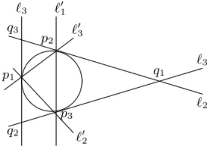
boundaryofX from the pointa. If one projectsX toPn−1from the pointa,

then the apparent boundary is the ramification divisor of the projection map. The following picture makes an attempt to show what happens in the case whenX is a conic.

a Pa(X)

X

Figure 1.1 Polar line of a conic

The set of first polarsPa(X)defines a linear system contained in the com-plete linear systemO_Pn(d−1). The dimension of this linear system≤n. We

will be freely using the language of linear systems and divisors on algebraic varieties (see [283]).

Proposition 1.1.6 The dimension of the linear system of first polars≤rif and only if, after a linear change of variables, the polynomialf becomes a polynomial inr+ 1variables.

Proof LetX =V(f). It is obvious that the dimension of the linear system of first polars≤rif and only if the linear mapE→Sd−1₍_E∨₎_{, v}_7→_D

v(f)has kernel of dimension≥n−r. Choosing an appropriate basis, we may assume that the kernel is generated by vectors(1,0, . . . ,0), etc. Now, it is obvious that

f does not depend on the variablest0, . . . , tn−r−1.

It follows from Theorem1.1.5that the first polarPa(X)of a pointawith respect to a hypersurfaceX passes through all singular points ofX. One can say more.

Proposition 1.1.7 Letabe a singular point ofXof multiplicitym. For each

r ≤degX−m,Par(X)has a singular point ataof multiplicitymand the

tangent cone ofPar(X)atacoincides with the tangent coneTCa(X)ofXat a. For any pointb 6=a, ther-th polarPbr(X)has multiplicity≥m−rata

and its tangent cone atais equal to ther-th polar ofTCa(X)with respect to

b.

(21)

assume thata= [1,0, . . . ,0]. ThenX =V(f), where

f =td₀−mfm(t1, . . . , tn) +t0d−m−1fm+1(t1, . . . , tn) +· · ·+fd(t1, . . . , tn). (1.15) The equationfm(t1, . . . , tn) = 0 defines the tangent cone of X at b. The equation ofPar(X)is

∂r_f

∂tr 0

=r! d−m−r

X

i=0

d−m−i r

td₀−m−r−ifm+i(t1, . . . , tn) = 0.

It is clear that[1,0, . . . ,0]is a singular point ofPar(X)of multiplicitymwith

the tangent coneV(fm(t1, . . . , tn)).

Now we prove the second assertion. Without loss of generality, we may assume thata = [1,0, . . . ,0]andb = [0,1,0, . . . ,0]. Then the equation of

Pbr(X)is

∂r_f

∂tr 1

=td₀−m∂

r_f m

∂tr 1

+· · ·+∂ r_f

d

∂tr 1

= 0.

The pointais a singular point of multiplicity≥m−r. The tangent cone of

Pbr(X)at the pointais equal to V(∂ r_f

m

∂tr

1 )and this coincides with the r-th

polar of TCa(X) =V(fm)with respect tob.

We leave it to the reader to see what happens ifr > d−m.

Keeping the notation from the previous proposition, consider a line`through the pointasuch that it intersectsXat some pointx6=awith multiplicity larger than one. The closure ECa(X)of the union of such lines is called the envelop-ing coneofX at the pointa. IfX is not a cone with vertex ata, the branch divisor of the projectionp:X\ {a} →_Pn−1_from_a_{is equal to the projection} of the enveloping cone. Let us find the equation of the enveloping cone.

As above, we assume thata= [1,0, . . . ,0]. LetHbe the hyperplanet0= 0. Write`in a parametric formua+vxfor somex∈H. Plugging in Equation (1.15), we get

P(t) =td−mfm(x1, . . . , xn)+td −m−1

fm+1(x1, . . . , xm)+· · ·+fd(x1, . . . , xn) = 0,

wheret=u/v.

We assume thatX 6= TCa(X), i.e.X is not a cone with vertex ata (oth-erwise, by definition, ECa(X) = TCa(X)). The image of the tangent cone under the projectionp: X\ {a} →H ∼=Pn−1is a proper closed subset of

(22)

poly-nomialP =A0Tk+· · ·+Akof degreek. Recall that

A0Dk(A0, . . . , Ak) = (−1)k(k−1)/2Res(P, P0)(A0, . . . , Ak), where Res(P, P0)is the resultant ofP and its derivativeP0. It follows from the known determinant expression of the resultant that

Dk(0, A1, . . . , Ak) = (−1)

k2−k+2 2 A2

0Dk−1(A1, . . . , Ak).

The equationP(t) = 0has a multiple zero witht6= 0if and only if Dd−m(fm(x), . . . , fd(x)) = 0.

So, we see that

ECa(X)⊂V(Dd−m(fm(x), . . . , fd(x))), (1.16)

ECa(X)∩TCa(X)⊂V(Dd−m−1(fm+1(x), . . . , fd(x))).

It follows from the computation of∂_∂trfr

0 in the proof of the previous Proposition

that the hypersurfaceV(Dd−m(fm(x), . . . , fd(x)))is equal to the projection

ofPa(X)∩XtoH.

SupposeV(Dd−m−1(fm+1(x), . . . , fd(x))) and TCa(X)do not share an

irreducible component. Then

V(Dd−m(fm(x), . . . , fd(x)))\TCa(X)∩V(Dd−m(fm(x), . . . , fd(x)))

=V(Dd−m(fm(x), . . . , fd(x)))\V(Dd−m−1(fm+1(x), . . . , fd(x)))⊂ECa(X),

gives the opposite inclusion of (1.16), and we get

ECa(X) =V(Dd−m(fm(x), . . . , fd(x))). (1.17) Note that the discriminantDd−m(A0, . . . , Ak)is an invariant of the group SL(2)in its natural representation on degreekbinary forms. Taking the diago-nal subtorus, we immediately infer that any monomialAi0

0 · · ·A ik

k entering in the discriminant polynomial satisfies

k

X

s=0

is= 2 k

X

s=0

sis.

It is also known that the discriminant is a homogeneous polynomial of degree 2k−2. Thus, we get

k(k−1) = k

X

s=0

(23)

In our casek=d−m, we obtain that

degV(Dd−m(fm(x), . . . , fd(x))) =

d−m

X

s=0

(m+s)is

=m(2d−2m−2) + (d−m)(d−m−1) = (d+m)(d−m−1).

This is the expected degree of the enveloping cone. Example1.1.8 Assumem=d−2, then

D2(fd−2(x), fd−1(x), fd(x)) =fd−1(x)2−4fd−2(x)fd(x),

D2(0, fd−1(x), fd(x)) =fd−2(x) = 0.

Supposefd−2(x)andfd−1are coprime. Then our assumption is satisfied, and we obtain

ECa(X) =V(fd−1(x)2−4fd−2(x)fd(x)).

Observe that the hypersurfacesV(fd−2(x))andV(fd(x))are everywhere

tan-gent to the enveloping cone. In particular, the quadric tantan-gent cone TCa(X)is everywhere tangent to the enveloping cone along the intersection ofV(fd−2(x)) withV(fd−1(x)).

For any nonsingular quadricQ, the mapx 7→ Px(Q)defines a projective isomorphism from the projective space to the dual projective space. This is a special case of a correlation.

According to classical terminology, a projective automorphism of Pn is

called acollineation. An isomorphism from|E|to its dual spaceP(E)is called

acorrelation. A correlationc:|E| →P(E)is given by an invertible linear map

φ:E →E∨defined uniquely up to proportionality. A correlation transforms points in|E|to hyperplanes in|E|. A pointx∈ |E|is calledconjugateto a pointy∈ |E|with respect to the correlationcify∈c(x). The transpose of the inverse mapt_φ−1_:_E∨_→_E_{transforms hyperplanes in}_|_E_|_{to points in}_|_E_|_{. It}

can be considered as a correlation between the dual spacesP(E)and|E|. It is

denoted byc∨and is called thedual correlation. It is clear that(c∨)∨ =c. If

H is a hyperplane in|E|andxis a point inH, then pointy ∈ |E|conjugate toxundercbelongs to any hyperplaneH0in|E|conjugate toH underc∨.

A correlation can be considered as a line in(E⊗E)∨spanned by a nonde-generate bilinear form, or, in other words as a nonsingular correspondence of type(1,1)in|E| × |E|. The dual correlation is the image of the divisor under the switch of the factors. A pair(x, y)∈ |E| × |E|of conjugate points is just a point on this divisor.

(24)

correlations form a groupΣPGL(E)isomorphic to the group of outer auto-morphisms of PGL(E). The subgroup of collineations is of index 2.

A correlationc of order 2 in the groupΣPGL(E)is called a polarity. In linear representative, this means thattφ=λφfor some nonzero scalarλ. After transposing, we obtainλ=±1. The caseλ= 1corresponds to the (quadric) polarity with respect to a nonsingular quadric in|E|which we discussed in this section. The caseλ=−1corresponds to anull-system(ornull polarity) which we will discuss in Chapters 2 and 10. In terms of bilinear forms, a correlation is a quadric polarity (resp. null polarity) if it can be represented by a symmetric (skew-symmetric) bilinear form.

Theorem 1.1.9 Any projective automorphism is equal to the product of two quadric polarities.

Proof Choose a basis inEto represent the automorphism by a Jordan matrix

J. LetJk(λ)be its block of sizekwithλat the diagonal. Let

Bk =



     

0 0 . . . 0 1 0 0 . . . 1 0

..

. ... ... ... ... 0 1 . . . 0 0 1 0 . . . 0 0



      .

Then

Ck(λ) =BkJk(λ) =



     

0 0 . . . 0 λ

0 0 . . . λ 1 ..

. ... ... ... ... 0 λ . . . 0 0

λ 1 . . . 0 0



      .

(25)

1.1.3 Polar quadrics

A(d−2)-polar ofX =V(f)is a quadric, called thepolar quadricofXwith respect toa= [a0, . . . , an]. It is defined by the quadratic form

q=D_ad−2(f) = X

|i|=d−2 d−2

i

ai∂if.

Using Equation (1.9), we obtain

q= X

|i|=2

₂

i

ti∂if(a).

By (1.14), each a ∈ X belongs to the polar quadricPad−2(X). Also, by

Theorem1.1.5,

Ta(Pad−2(X)) =P_a(P_ad−2(X)) =P_ad−1(X) =_T_a(X). (1.18)

This shows that the polar quadric is tangent to the hypersurface at the pointa. Consider the line` = ab through two points a, b. Let ϕ : _P1 _→

Pn be

its parametric equation, i.e. a closed embedding with the image equal to`. It follows from (1.8) and (1.9) that

i(X, ab)a ≥s+ 1⇐⇒b∈Pad−k(X), k≤s. (1.19)

Fors = 0, the condition means thata∈ X. Fors = 1, by Theorem 1.1.5, this condition implies thatb, and hence`, belongs to the tangent planeTa(X).

Fors= 2, this condition implies thatb ∈P_ad−2(X). Since`is tangent toX

ata, andPad−2(X)is tangent toXata, this is equivalent to that`belongs to Pad−2(X).

It follows from (1.19) thatais a singular point ofX of multiplicity≥s+ 1 if and only ifPad−k(X) = _Pn for k ≤ s. In particular, the quadric polar Pad−2(X) =_Pnif and only ifais a singular point ofXof multiplicity≥3.

Definition 1.1.10 A line is called aninflection tangenttoXat a pointaif

i(X, `)a>2.

Proposition 1.1.11 Let`be a line through a pointa. Then`is an inflection tangent toXataif and only if it is contained in the intersection ofTa(X)with the polar quadricPad−2(X).

Note that the intersection of an irreducible quadric hypersurfaceQ=V(q) with its tangent hyperplaneHat a pointa∈Qis a cone inHover the quadric

¯

(26)

Corollary 1.1.12 Assumen≥3. For anya∈ X, there exists an inflection tangent line. The union of the inflection tangents containing the pointais the coneTa(X)∩Pad−2(X)in_Ta(X).

Example1.1.13 Assumeais a singular point ofX. By Theorem1.1.5, this is equivalent to thatPad−1(X) =_Pn. By (1.18), the polar quadricQis also

singular ataand therefore it must be a cone over its image under the projection froma. The union of inflection tangents is equal toQ.

Example1.1.14 Assumeais a nonsingular point of an irreducible surfaceX

inP3. A tangent hyperplaneTa(X)cuts out inX a curveC with a singular

pointa. Ifais an ordinary double point ofC, there are two inflection tangents corresponding to the two branches ofCata. The polar quadricQis nonsingu-lar ata. The tangent cone ofCat the pointais a cone over a quadricQ¯in_P1_. IfQ¯consists of two points, there are two inflection tangents corresponding to the two branches ofCata. IfQ¯ consists of one point (corresponding to non-reduced hypersurface inP1), then we have one branch. The latter case happens

only ifQis singular at some pointb6=a.

1.1.4 The Hessian hypersurface

LetQ(a)be the polar quadric ofX=V(f)with respect to some pointa∈Pn.

The symmetric matrix defining the corresponding quadratic form is equal to theHessian matrixof second partial derivatives off

He(f) = ∂ 2_f

∂ti∂tj

i,j=0,...,n,

evaluated at the pointa.The quadricQ(a)is singular if and only if the deter-minant of the matrix is equal to zero (the locus of singular points is equal to the projectivization of the null-space of the matrix). The hypersurface

He(X) =V(detHe(f))

describes the set of points a ∈ Pn such that the polar quadricPad−2(X)is

singular. It is called theHessian hypersurfaceofX. Its degree is equal to(d− 2)(n+ 1)unless it coincides withPn.

Proposition 1.1.15 The following is equivalent:

(i) He(X) =_Pn_;

(ii) there exists a nonzero polynomialg(z0, . . . , zn)such that

(27)

Proof This is a special case of a more general result about theJacobian de-terminant (also known as the functional determinant) ofn+ 1 polynomial functionsf0, . . . , fndefined by

J(f0, . . . , fn) = det (

∂fi

∂tj )

.

SupposeJ(f0, . . . , fn)≡0. Then the mapf :Cn+1 →Cn+1defined by the

functionsf0, . . . , fn is degenerate at each point (i.e.dfxis of rank< n+ 1 at each pointx). Thus the closure of the image is a proper closed subset of

Cn+1. Hence there is an irreducible polynomial that vanishes identically on

the image.

Conversely, assume thatg(f0, . . . , fn) ≡ 0 for some polynomialgwhich we may assume to be irreducible. Then

∂g ∂ti

= n

X

j=0

∂g ∂zj

(f0, . . . , fn)

∂fj

∂ti

= 0, i= 0, . . . , n.

Sincegis irreducible, its set of zeros is nonsingular on a Zariski open setU. Thus the vector

∂g ∂z0

(f0(x), . . . , fn(x)), . . . , ∂g ∂zn

(f0(x), . . . , fn(x)

is a nontrivial solution of the system of linear equations with matrix(∂fi

∂tj(x)),

wherex∈U. Therefore, the determinant of this matrix must be equal to zero. This implies thatJ(f0, . . . , fn) = 0onU, hence it is identically zero. Remark1.1.16 It was claimed by O. Hesse that the vanishing of the Hessian implies that the partial derivatives are linearly dependent. Unfortunately, his attempted proof was wrong. The first counterexample was given by P. Gordan and M. Noether in [254]. Consider the polynomial

f =t2t20+t3t21+t4t0t1.

Note that the partial derivatives

∂f ∂t2

=t2₀, ∂f ∂t3

=t2₁, ∂f ∂t4

=t0t1

are algebraically dependent. This implies that the Hessian is identically equal to zero. We have

∂f ∂t0

= 2t0t2+t4t1,

∂f ∂t1

= 2t1t3+t4t0.

Suppose that a linear combination of the partials is equal to zero. Then

(28)

Collecting the terms in whicht2, t3, t4enter, we get

2c3t0= 0, 2c4t1= 0, c3t1+c4t0= 0.

This givesc3 = c4 = 0. Since the polynomialst02, t21, t0t1are linearly inde-pendent, we also getc0=c1=c2= 0.

The known cases when the assertion of Hesse is true ared= 2(anyn) and

n≤3(anyd) (see [254], [371], [103]).

Recall that the set of singular quadrics inPnis thediscriminant

hypersur-faceD2(n)inPn(n+3)/2defined by the equation

det



   

t00 t01 . . . t0n

t01 t11 . . . t1n ..

. ... ... ...

t0n t1n . . . tnn



   

= 0.

By differentiating, we easily find that its singular points are defined by the determinants ofn×nminors of the matrix. This shows that the singular locus ofD2(n)parameterizes quadrics defined by quadratic forms of rank≤n−1 (or corank≥2). Abusing the terminology, we say that a quadricQis of rank

kif the corresponding quadratic form is of this rank. Note that dimSing(Q) =corankQ−1.

Assume that He(f) 6= 0. Consider the rational mapp : |E| → |S2₍_E∨₎_|

defined bya 7→ Pad−2(X). Note thatP_ad−2(f) = 0impliesP_ad−1(f) = 0

and hencePn

i=0bi∂if(a) = 0for allb. This shows thatais a singular point ofX. Thuspis defined everywhere except maybe at singular points ofX. So the mappis regular ifXis nonsingular, and the preimage of the discriminant hypersurface is equal to the Hessian ofX. The preimage of the singular locus Sing(D2(n))is the subset of pointsa∈He(f)such that Sing(Pad−2(X))is of

positive dimension.

Here is another description of the Hessian hypersurface.

Proposition 1.1.17 The Hessian hypersurfaceHe(X)is the locus of singular points of the first polars ofX.

Proof Leta∈He(X)and letb∈Sing(Pad−2(X)). Then Db(Dad−2(f)) =D_ad−2(Db(f)) = 0.

SinceDb(f)is of degreed−1, this means thatTa(Pb(X)) =Pn, i.e.,ais a

(29)

Conversely, ifa∈Sing(Pb(X)), thenDad−2(Db(f)) = Db(D_ad−2(f)) =

0. This means thatbis a singular point of the polar quadric with respect toa. Hencea∈He(X).

Let us find the affine equation of the Hessian hypersurface. Applying the Euler formula (1.13), we can write

t0f0i= (d−1)∂if −t1f1i− · · · −tnfni,

t0∂0f =df−t1∂1f− · · · −tn∂nf,

wherefij denote the second partial derivative. Multiplying the first row of the Hessian determinant byt0 and adding to it the linear combination of the remaining rows taken with the coefficientsti, we get the following equality:

det(He(f)) = d−1

t0 det     

∂0f ∂1f . . . ∂nf

f10 f11 . . . f1n ..

. ... ... ...

fn0 fn1 . . . fnn

     .

Repeating the same procedure but this time with the columns, we finally get

det(He(f)) = (d−1) 2 t2 0 det      d

d−1f ∂1f . . . ∂nf

∂1f f11 . . . f1n ..

. ... ... ...

∂nf fn1 . . . fnn

     . (1.20)

Letφ(z1, . . . , zn)be the dehomogenization offwith respect tot0, i.e.,

f(t0, . . . , td) =td0φ(

t1

t0

, . . . ,tn t0

).

We have

∂f ∂ti

=td₀−1φi(z1, . . . , zn),

∂2_f

∂ti∂tj

=td₀−2φij(z1, . . . , zn), i, j= 1, . . . , n,

where

φi=

∂φ ∂zi

, φij=

∂2_φ

∂zi∂zj

.

(30)

factor,

t−₀(n+1)(d−2)det(He(φ)) = det



   

d

d−1φ(z) φ1(z) . . . φn(z)

φ1(z) φ11(z) . . . φ1n(z) ..

. ... ... ...

φn(z) φn1(z) . . . φnn(z)



    ,

(1.21) wherez= (z1, . . . , zn), zi=ti/t0, i= 1, . . . , n.

Remark1.1.18 Iff(x, y)is a real polynomial in three variables, the value of (1.21) at a pointv∈Rnwith[v]∈V(f)multiplied byf1(a)2+f2−(a)12+f3(a)2 is

equal to theGauss curvatureofX(_R)at the pointa(see [222]).

1.1.5 Parabolic points

Let us see where He(X)intersectsX. We assume that He(X)is a hypersurface of degree(n+ 1)(d−2) >0. A glance at the expression (1.21) reveals the following fact.

Proposition 1.1.19 Each singular point ofX belongs toHe(X).

Let us see now when a nonsingular pointa∈ X lies in its Hessian hyper-surface He(X).

By Corollary1.1.12, the inflection tangents inTa(X)sweep the intersection

of _Ta(X)with the polar quadric Pad−2(X). Ifa ∈ He(X), then the polar

quadric is singular at some pointb.

Ifn= 2, a singular quadric is the union of two lines, so this means that one of the lines is an inflection tangent. A pointaof a plane curveX such that there exists an inflection tangent atais called aninflection pointofX.

Ifn >2, the inflection tangent lines at a pointa∈X∩He(X)sweep a cone over a singular quadric inPn−2 (or the wholePn−2if the point is singular).

Such a point is called aparabolic pointofX. The closure of the set of parabolic points is theparabolic hypersurfaceinX(it could be the wholeX).

Theorem 1.1.20 LetX be a hypersurface of degreed >2inPn. Ifn= 2,

thenHe(X)∩Xconsists of inflection points ofX. In particular, each nonsin-gular curve of degree≥3has an inflection point, and the number of inflections points is either infinite or less than or equal to3d(d−2). Ifn >2, then the setX∩He(X)consists of parabolic points. The parabolic hypersurface inX

is either the wholeXor a subvariety of degree(n+ 1)d(d−2)inPn.

Example 1.1.21 Let X be a surface of degreedinP3. If ais a parabolic

(31)

multiplicity higher than 3 or it has only one branch. In fact, otherwiseX has at least two distinct inflection tangent lines which cannot sweep a cone over a singular quadric inP1. The converse is also true. For example, a nonsingular

quadric has no parabolic points, and all nonsingular points of a singular quadric are parabolic.

A generalization of a quadratic cone is adevelopable surface. It is a special kind of aruled surfacewhich characterized by the condition that the tangent plane does not change along a ruling. We will discuss these surfaces later in Chapter 10. The Hessian surface of a developable surface contains this surface. The residual surface of degree2d−8 is called thepro-Hessian surface. An example of a developable surface is the quartic surface

(t0t3−t1t2)2−4(t21−t0t2)(t22−t1t3) =−6t0t1t2t3+4t31t3+4t0t32+t 2 0t

2 3−3t

2 1t

2 2 = 0.

It is the surface swept out by the tangent lines of a rational normal curve of degree 3. It is also thediscriminant surfaceof a binary cubic, i.e. the surface parameterizing binary cubicsa0u3+ 3a1u2v+ 3a2uv2+a3v3with a multiple root. The pro-Hessian of any quartic developable surface is the surface itself [84].

Assume now thatX is a curve. Let us see when it has infinitely many in-flection points. Certainly, this happens whenX contains a line component; each of its points is an inflection point. It must be also an irreducible compo-nent of He(X). The set of inflection points is a closed subset ofX. So, ifX

has infinitely many inflection points, it must have an irreducible component consisting of inflection points. Each such component is contained in He(X). Conversely, each common irreducible component ofXand He(X)consists of inflection points.

We will prove the converse in a little more general form taking care of not necessarily reduced curves.

Proposition 1.1.22 A polynomialf(t0, t1, t2)divides its Hessian polynomial He(f)if and only if each of its multiple factors is a linear polynomial. Proof Since each point on a non-reduced component ofXred⊂V(f)is a

(32)

Thus the equation ofRlooks like

f(x, y) =y−xr+g(x, y), (1.22) whereg(x, y)does not contain termscy, c ∈_C. It is easy to see that(0,0)is an inflection point if and only ifr >2with the inflection tangenty= 0.

We use the affine equation of the Hessian (1.21), and obtain that the image of

h(x, y) = det





d

d−1f f1 f2

f1 f11 f12

f2 f21 f22





inC[[t]]is equal to

det





0 −rtr−1₊_g

1 1 +g2

−rtr−1₊_g

1 −r(r−1)tr−2+g11 g12

1 +g2 g12 g22



.

Since every monomial entering ingis divisible byy2_{, xy}_or_xi_{, i > r}_{, we} see that _∂y∂g is divisible bytand ∂g_∂x is divisible bytr−1. Alsog11is divisible bytr−1_{. This shows that}

h(x, y) = det





0 atr−1₊_{· · ·} _{1 +}_{· · ·}

atr−1+· · · −r(r−1)tr−2+· · · g12 1 +· · · g12 g22



,

where· · · denotes terms of higher degree int. We compute the determinant and see that it is equal tor(r−1)tr−2+· · ·. This means that its image in

C[[t]]is not equal to zero, unless the equation of the curve is equal toy = 0,

i.e. the curve is a line.

In fact, we have proved more. We say that a nonsingular point ofXis an in-flection point oforderr−2and denote the order by ordflxXif one can choose an equation of the curve as in (1.22) withr≥3. It follows from the previous proof thatr−2is equal to the multiplicityi(X,He)xof the intersection of the curve and its Hessian at the pointx. It is clear that ordflxX =i(`, X)x−2, where`is the inflection tangent line ofX atx. IfXis nonsingular, we have

X

x∈X

i(X,He)x= X x∈X

ordflxX = 3d(d−2). (1.23)

1.1.6 The Steinerian hypersurface

(33)

hypersurfaceSt(X)ofXis the locus of singular points of the polar quadrics. Thus

St(X) = [ a∈He(X)

Sing(Pad−2(X)). (1.24)

The proof of Proposition 1.1.17shows that it can be equivalently defined as St(X) ={a∈Pn:Pa(X)is singular}. (1.25) We also have

He(X) = [

a∈St(X)

Sing(Pa(X)). (1.26)

A pointb= [b0, . . . , bn]∈St(X)satisfies the equation

He(f)(a)·



 

b0 .. .

bn





= 0, (1.27)

wherea∈He(X). This equation defines a subvariety

HS(X)⊂Pn×Pn (1.28)

given byn+ 1equations of bidegree(d−2,1).

The following argument confirms our expectation. It is known (see, for ex-ample, [240]) that the locus of singular hypersurfaces of degreedin|E|is a hypersurface

Dd(n)⊂ |Sd(E∨)|

of degree(n+ 1)(d−1)n defined by thediscriminantof a general degreed

homogeneous polynomial inn+ 1variables (thediscriminant hypersurface). LetLbe the projective subspace of|Sd−1₍_E∨₎_|_{that consists of first polars of} X. Assume that no polarPa(X)is equal toPn. Then

St(X)∼=L∩Dn(d−1).

So, unlessLis contained inDn(d−1), we get a hypersurface. Moreover, we obtain

deg(St(X)) = (n+ 1)(d−2)n. (1.29)

Assume that the quadric Pad−2(X) is of corank 1. Then it has a unique

(34)

St(X)coincides with the image of the Hessian hypersurface under the rational map

st:He(X)_99KSt(X), a7→Sing(P_ad−2(X)),

given by polynomials of degreen(d−2). We call it theSteinerian map. Of course, it is not defined when all polar quadrics are of corank > 1. Also, if the first polar hypersurfacePa(X)has an isolated singular point for a general pointa, we get a rational map

st−1:St(X)_99KHe(X), a7→Sing(Pa(X)).

These maps are obviously inverse to each other. It is a difficult question to determine the sets of indeterminacy points for both maps.

Proposition 1.1.23 LetXbe a reduced hypersurface. The Steinerian hyper-surface ofX coincides withPnifX has a singular point of multiplicity≥3.

The converse is true if we additionally assume thatXhas only isolated singu-lar points.

Proof Assume thatX has a point of multiplicity≥ 3. We may harmlessly assume that the point isp= [1,0, . . . ,0]. Write the equation ofXin the form

f =tk₀gd−k(t1, . . . , tn) +tk0−1gd−k+1(t1, . . . , tn) +· · ·+gd(t1, . . . , tn) = 0, (1.30) where the subscript indicates the degree of the polynomial. Since the multi-plicity ofpis greater than or equal to3, we must haved−k≥3. Then a first polarPa(X)has the equation

a0 k

X

i=0

(k−i)t₀k−1−igd−k+i+ n

X

s=1

as k

X

i=0

tk₀−i∂gd−k+i ∂ts

= 0. (1.31)

It is clear that the pointpis a singular point ofPa(X)of multiplicity≥d−

k−1≥2.

Conversely, assume that all polars are singular. By Bertini’s Theorem (see [279], Theorem 17.16), the singular locus of a general polar is contained in the base locus of the linear system of polars. The latter is equal to the singular locus ofX. By assumption, it consists of isolated points, hence we can find a singular point ofX at which a general polar has a singular point. We may assume that the singular point isp= [1,0, . . . ,0]and (1.30) is the equation of

X. Then the first polarPa(X)is given by Equation (1.31). The largest power of

(35)

Example1.1.24 The assumption on the singular locus is essential. First, it is easy to check thatX =V(f2_{), where}_V₍_f₎_{is a nonsingular hypersurface has} no points of multiplicity≥3and its Steinerian coincides withPn. An example

of a reduced hypersurfaceXwith the same property is a surface of degree 6 in

P3given by the equation

( 3

X

i=0

t3i) 2

+ ( 3

X

i=0

t2i) 3

= 0.

Its singular locus is the curveV(P3

i=0t 3 i)∩V(

P3

i=0t 2

i).Each of its points is a double point onX. Easy calculation shows that

Pa(X) =V ( 3

X

i=0

t3_i) 3

X

i=0

ait2i + ( 3

X

i=0

t2_i)2 3

X

i=0

aiti

. and V( 3 X i=0

t3i)∩V( 3

X

i=0

t2i)∩V( 3

X

i=0

ait2i)⊂Sing(Pa(X)).

By Proposition1.1.7, Sing(X)is contained in St(X). Since the same is true for He(X), we obtain the following.

Proposition 1.1.25 The intersectionHe(X)∩St(X)contains the singular locus ofX.

One can assign one more variety to a hypersurfaceX =V(f). This is the Cayleyan variety. It is defined as the image Cay(X)of the rational map

HS(X)_99KG1(Pn), (a, b)7→ab,

whereGr(Pn)denotes the Grassmannian ofr-dimensional subspaces inPn.

Note that in the casen= 2, the Cayleyan variety is a plane curve in the dual plane, theCayleyan curveofX.

Proposition 1.1.26 LetXbe a general hypersurface of degreed≥3. Then

degCay(X) =

(_P_n

i=1(d−2) i n+1

i

n−1 i−1

ifd >3,

1 2 Pn i=1 n+1 i

n−1 i−1

ifd= 3,

where the degree is considered with respect to the Pl¨ucker embedding of the GrassmannianG1(Pn).

Proof Since St(X) 6= Pn,the correspondence HS(X)is a complete

(36)

a∈ Sing(Pa(X))implies thata∈Sing(X), the intersection of HS(X)with the diagonal is empty. Consider the regular map

r:HS(X)→G1(Pn), (a, b)7→ab. (1.32)

It is given by the linear system of divisors of type(1,1)onPn×Pnrestricted

to HS(X). The genericity assumption implies that this map is of degree 1 onto the image ifd > 3 and of degree 2 ifd = 3 (in this case the map factors through the involution ofPn×Pnthat switches the factors).

It is known that the set of lines intersecting a codimension 2 linear sub-space Λis a hyperplane section of the GrassmannianG1(Pn)in its Pl¨ucker

embedding. Write_Pn₌_|_E_|_and_{Λ =}_|_L_|_{. Let}_ω ₌_v

1∧. . .∧vn−1for some basis(v1, . . . , vn−1)ofL. The locus of pairs of points(a, b) = ([w1],[w2])in

Pn×Pnsuch that the lineabintersectsΛis given by the equationw1∧w2∧ω= 0.This is a hypersurface of bidegree(1,1)inPn×Pn. This shows that the map

(1.32) is given by a linear system of divisors of type(1,1). Its degree (or twice of the degree) is equal to the intersection((d−2)h1+h2)n+1(h1+h2)n−1, whereh1, h2are the natural generators ofH2(Pn×Pn,Z). We have

((d−2)h1+h2)n+1(h1+h2)n−1=

n+1

X

i=0 n+1

i

(d−2)ihi₁hn+1₂ −i

n−1

X

j=0 n−1

j

hn₁−1−jhj₂

= n

X

i=1

(d−2)i n+1_i n−1 i−1

.

For example, ifn= 2, d >3, we obtain a classical result degCay(X) = 3(d−2) + 3(d−2)2= 3(d−2)(d−1),

anddegCay(X) = 3ifd= 3.

Remark1.1.27 The homogeneous forms defining the Hessian and Steinerian hypersurfaces ofV(f)are examples ofcovariantsoff. We already discussed them in the casen= 1. The form defining the Cayleyan of a plane curve is an example of acontravariantoff.

1.1.7 The Jacobian hypersurface

(37)

to arbitraryn-dimensional linear systems of hypersurfaces inPn = |E|. We

assume that the linear system has no fixed components, i.e. its general member is an irreducible hypersurface of some degreed. LetL⊂Sd(E∨)be a linear subspace of dimensionn+ 1and|L|be the corresponding linear system of hypersurfaces of degreed. Note that, in the case of linear system of polars of a hypersurfaceXof degreed+ 1, the linear subspaceLcan be canonically iden-tified withEand the inclusion|E| ⊂ |Sd₍_E∨₎_|_{corresponds to the polarization}

mapa7→Pa(X).

LetDd(n)⊂ |Sd(E∨)|be the discriminant hypersurface. D(|L|) =|L| ∩Dd(n)

is called thediscriminant hypersurfaceof|L|.

e

D(|L|) ={(x, D)∈_Pn_{× |}_L_|_:_x_∈_Sing(_D₎_}

with two projectionsp:De →D(|L|)andq:De → |L|. We define theJacobian

hypersurfaceof|L|as

Jac(|L|) =q(D(e |L|)).

It parameterizes singular points of singular members of|L|. Again, it may co-incide with the wholePn. In the case of polar linear systems, the discriminant

hypersurface is equal to the Steinerian hypersurface, and the Jacobian hyper-surface is equal to the Hessian hyperhyper-surface.

TheSteinerian hypersurfaceSt(|L|)x∈ ∩D∈|L|Pan−1(D). SincedimL= n+ 1, the intersection is empty, unless there existsDsuch thatPan−1(D) = 0.

ThusPan(D) = 0anda ∈ Sing(D), hence a ∈ Jac(|L|)andD ∈ D(|L|).

Conversely, ifa∈Jac(|L|), then∩D∈|L|Pan−1(D)6=∅and it is contained in

St(|L|). By duality (1.12),

x∈ \

D∈|L|

Pan−1(D)⇔a∈ \

D∈|L| Px(D).

Thus the Jacobian hypersurface is equal to the locus of points which belong to the intersection of the first polars of divisors in|L|with respect to some point

x∈St(X). Let

HS(|L|) ={(a, b)∈He(|L|)×St(|L|) :a∈ \ D∈|L|

Pb(D)}

={(a, b)∈He(|L|)×St(|L|) :b∈ \ D∈|L|

(38)

It is clear that HS(|L|)⊂Pn×Pnis a complete intersection ofn+ 1divisors

of type(d−1,1). In particular,

ωHS(|L|)∼=pr∗1(OPn((d−2)(n+ 1))). (1.33) One expects that, for a general pointx∈St(|L|), there exists a uniquea∈ Jac(|L|)and a uniqueD ∈ D(|L|)as above. In this case, the correspondence HS(|L|)defines a birational isomorphism between the Jacobian and Steinerian hypersurface. Also, it is clear that He(|L|) =St(|L|)ifd= 2.

Assume that |L| has no base points. Then HS(|L|) does not intersect the diagonal ofPn×Pn. This defines a map

HS(|L|)→G1(Pn), (a, b)7→ab.

Its image Cay(|L|)is called theCayleyan varietyof|L|.

A line`∈Cay(|L|)is called aReye lineof|L|. It follows from the defini-tions that a Reye line is characterized by the property that it contains a point such that there is a hyperplane in|L|of hypersurfaces tangent to`at this point. For example, ifd= 2this is equivalent to the property that`is contained is a linear subsystem of|L|of codimension 2 (instead of expected codimension 3). The proof of Proposition 1.1.26 applies to our more general situation to give the degree of Cay(|L|)for a generaln-dimensional linear system|L|of hypersurfaces of degreed.

degCay(|L|) =

(_Pn

i=1(d−1) i n+1

i

n−1 i−1

ifd >2,

1 2

Pn

i=1 n+1

i

n−1 i−1

ifd= 2. (1.34)

Letf = (f0, . . . , fn)be a basis of L. Choose coordinates in Pn to

iden-tifySd₍_E∨₎_{with the polynomial ring}

C[t0, . . . , tn]. A well-known fact from the complex analysis asserts that Jac(|L|)is given by the determinant of the Jacobian matrix

J(f) =



   

∂0f0 ∂1f0 . . . ∂nf0

∂0f1 ∂1f1 . . . ∂nf1 ..

. ... ... ...

∂0fn ∂1fn . . . ∂nfn



    .

In particular, we expect that

degJac(|L|) = (n+ 1)(d−1).

Ifa∈Jac(|L|), then a nonzero vector in the null-space ofJ(f)defines a point

xsuch thatPx(f0)(a) =. . .=Px(fn)(a) = 0. Equivalently,

(39)

This shows that St(|L|)is equal to the projectivization of the union of the null-spaces Null(Jac(f(a))), a∈_Cn+1_{. Also, a nonzero vector in the null space of} the transpose matrixtJ(f)defines a hypersurface inD(|L|)with singularity at the pointa.

Let Jac(|L|)0_{be the open subset of points where the corank of the jacobian} matrix is equal to 1. We assume that it is a dense subset of Jac(|L|). Then, taking the right and the left kernels of the Jacobian matrix, defines two maps

Jac(|L|)0→D(|L|), Jac(|L|)0→St(|L|).

Explicitly, the maps are defined by the nonzero rows (resp. columns) of the adjugate matrix adj(He(f)).

Letφ_|L|:Pn99K|L∨|be the rational map defined by the linear system|L|.

Under some assumptions of generality which we do not want to spell out, one can identify Jac(|L|)with the ramification divisor of the map andD(|L|)with the dual hypersurface of the branch divisor.

Let us now define a new variety attached to an-dimensional linear system inPn. Consider the inclusion mapL ,→Sd(E∨)and let

L ,→Sd(E)∨, f 7→f ,˜

be the restriction of the total polarization map (1.2) toL. Now we can consider |L|as an-dimensional linear system|fL|on|E|dof divisors of type(1, . . . ,1).

Let

PB(|L|) = \ D∈|fL|

D⊂ |E|d

be the base scheme of|fL|. We call it thepolar base locusof|L|. It is equal to

the complete intersection ofn+ 1effective divisors of type(1, . . . ,1). By the adjunction formula,

ωPB(|L|)=∼OPB(|L|).

If smooth, PB(|L|)is aCalabi-Yau varietyof dimension(d−1)n−1. For anyf ∈L, letN(f)be the set of pointsx= ([v(1)_]_{, . . . ,}_[_v(d)_])_{∈ |}_E_|d such that

˜

f(v(1), . . . , v(j−1), v, v(j+1), . . . , v(d)) = 0

for everyj= 1, . . . , dandv∈E. Since ˜

f(v(1), . . . , v(j−1), v, v(j+1), . . . , v(d)) =D_v(1)_···_v(j−1)_v(j+1)_···_v(d)(Dv(f)),

This can be also expressed in the form

g

(40)

Choose coordinatesu0, . . . , uninLand coordinatest0, . . . , tninE. Let˜fbe the image of a basisf ofLin(E∨)d_{. Then PB(}_|_L_|₎_{is a subvariety of}₍

Pn)d

given by a system ofdmultilinear equations ˜

f0(t(1), . . . , t(d)) =. . .= ˜fn(t(1), . . . , t(d)) = 0,

wheret(j) _{= (}_t(j) 0 , . . . , t

(j)

n ), j = 1, . . . , d. For anyλ = (λ0, . . . , λn), set ˜

fλ=P n i=0λif˜i.

Proposition 1.1.28 The following is equivalent:

(i) x∈PB(|L|)is a singular point, (ii) x∈N( ˜fλ)for someλ6= 0.

Proof The variety PB(|L|)is smooth at a pointxif and only if the rank of thed(n+ 1)×(n+ 1)-size matrix

(akij) =

∂f˜k

∂t(j)_i

(x)_{i,k=0,...,n,j=1,...,d}

is equal to n+ 1. Letf˜u = u0f˜0 +· · ·+unf˜n, whereu0, . . . , un are un-knowns. Then the nullspace of the matrix is equal to the space of solutions

u= (λ0, . . . , λn)of the system of linear equations

∂f˜u

∂u0

(x) =. . .= ∂ ˜

fu

∂un

(x) = ∂ ˜

fu

∂t(j)_i

(x) = 0. (1.36)

For a fixedλ, in terminology of [240], p. 445, the system has a solutionxin |E|d_if_f˜

λ=Pλif˜iis adegenerate multilinear form. By Proposition 1.1 from Chapter 14 of loc.cit.,f˜λis degenerate if and only ifN( ˜fλ)is non-empty. This proves the assertion.

For any non-empty subset I of{1, . . . , d}, let∆I be the subset of points

x∈ |E|d_{with equal projections to}_i_{-th factors with}_i_∈_I_{. Let}_∆k_{be the union} of∆Iwith#I=k. The set∆dis denoted by∆(the small diagonal).

Observe that PB(|L|) =HS(|L|)ifd= 2and PB(|L|)∩∆d−1consists of

dcopies isomorphic to HS(|L|)ifd >2.

Definition 1.1.29 An-dimensional linear system|L| ⊂ |Sd₍_E∨₎_|_{is called}

regularifPB(|L|)is smooth at each point of∆d−1. Proposition 1.1.30 Assume|L|is regular. Then

(41)

Proof (i) Assume thatx= ([v0], . . . ,[v0])∈PB(|L|)∩∆. Consider the lin-ear mapL→Edefined by evaluatingf˜at a point(v0, . . . , v0, v, v0, . . . , v0), wherev ∈E. This map factors through a linear mapL→E/[v0], and hence has a nonzerof in its kernel. This implies thatx ∈ N(f), and hencexis a singular point of PB(|L|).

(ii) In coordinates, the varietyD(e |L|)is a subvariety of type(1, d−1)of

Pn×Pngiven by the equations

n X k=0 uk ∂fk ∂t0 =. . .= n X k=0 uk ∂fk ∂tn = 0.

The tangent space at a point([λ],[a])is given by the system ofn+ 1linear equations in2n+ 2variables(X0, . . . , Xn, Y0, . . . , Yn)

n

X

k=0

∂fk

∂ti

(a)Xk+ n

X

j=0

∂2_f λ

∂ti∂tj

(a)Yj= 0, i= 0, . . . , n, (1.37)

where fλ = P n

k=0λkfk. Suppose ([λ],[a]) is a singular point. Then the equations are linearly dependent. Thus there exists a nonzero vector v = (α0, . . . , αn)such that

n X i=0 αi ∂fk ∂ti

(a) =Dv(fk)(a) = ˜fk(a, . . . , a, v) = 0, k= 0, . . . , n

and n

X

i

αi

∂2_f λ

∂ti∂tj

(a) =Dv(∂fλ

∂tj

)(a) =Dad−2_v( ∂fλ

∂tj

) = 0, j= 0, . . . , n,

wherefλ = Pλkfk. The first equation implies that x = ([a], . . . ,[a],[v]) belongs to PB(|L|). Since a ∈ Sing(fλ), we have Dad−1(∂f_∂tλ

j) = 0, j =

0, . . . , n. By (1.35), this and the second equation now imply thatx∈N(fλ). By Proposition1.1.28, PB(|L|)is singular atx, contradicting the assumption.

Corollary 1.1.31 Suppose|L|is regular. Then the projection

q:D(e |L|)→D(|L|)

is a resolution of singularities.

Consider the projectionp: D(e |L|) → Jac(|L|),(D, x) 7→x. Its fibres are

(42)

point. This implies that the morphismphas positive dimensional fibres. This simple observation gives the following.

Proposition 1.1.32 SupposeD(|L|)does not contain lines. ThenD(e |L|)is

smooth if and only if Jac(|L|)is smooth. Moreover, HS(|L|) ∼= St(|L|) ∼= Jac(|L|).

Remark1.1.33 We will prove later in Example1.2.3that the tangent space of the discriminant hypersurfaceDd(n)at a point corresponding to a hypersurface

X = V(f)with only one ordinary double pointxis naturally isomorphic to the linear space of homogeneous forms of degreedvanishing at the pointx

moduloCf. This implies thatD(|L|)is nonsingular at a point corresponding

to a hypersurface with one ordinary double point unless this double point is a base point of|L|. If|L|has no base points, the singular points ofD(|L|)are of two sorts: either they correspond to divisors with worse singularities than one ordinary double point, or the linear space |L|is tangent to Dd(n)at its nonsingular point.

Consider the natural action of the symmetric groupSd on(Pn)d. It leaves

PB(|L|)invarian. The quotient variety

Rey(|L|) =PB(|L|)/Sd

is called the Reye varietyof |L|. If d > 2 andn > 1, the Reye variety is singular.

Example1.1.34 Assumed = 2. Then PB(|L|) = HS(|L|)and Jac(|L|) = St(|L|). Moreover, Rey(|L|)∼=Cay(|L|). We have

degJac(|L|) = degD(|L|) =n+ 1, degCay(|L|) = n

X

i=1 n+1

i

n−1 i−1

.

The linear system is regular if and only if PB(|L|)is smooth. This coincides with the notion of regularity of a web of quadrics inP3discussed in [133].

A Reye line` is contained in a codimension 2 subspaceΛ(`)of|L|, and is characterized by this condition. The linear subsystem Λ(`) of dimension

n−2contains`in its base locus. The residual component is a curve of degree 2n−1−1which intersects`at two points. The points are the two ramification points of the pencilQ∩`, Q∈ |L|. The two singular points of the base locus of Λ(`) define two singular points of the intersection Λ(`)∩D(|L|). Thus Λ(`)is a codimension 2 subspace of|L|which is tangent to the determinantal hypersurface at two points.

Classical Algebraic Geometry: A Modern View - Free Computer, Programming, Mathematics, Technical Books, Lecture Notes and Tutorials