Maximum
likelihood
estimation
for
semiparametric
regression
models
with
multivariate
interval-censored
data
BYDONGLINZENG,FEIGAOANDD.Y.LIN
DepartmentofBiostatistics,CB#7420,UniversityofNorthCarolina,ChapelHill,
NorthCarolina27599,U.S.A.
[email protected] [email protected] [email protected]
SUMMARY
Interval-censoredmultivariatefailuretimedataarisewhentherearemultipletypesoffailure or thereisclustering ofstudysubjectsand eachfailuretime is knownonly tolie in acertain interval.Weinvestigatetheeffectsofpossiblytime-dependentcovariatesonmultivariatefailure timesbyconsideringabroadclassofsemiparametrictransformationmodelswithrandomeffects, andwe studynonparametricmaximumlikelihoodestimationunder general interval-censoring schemes.Weshowthattheproposedestimatorsforthefinite-dimensionalparametersare consis-tentandasymptoticallynormal,withalimitingcovariancematrixthatattainsthesemiparametric efficiency boundandcanbeconsistentlyestimatedthrough profilelikelihood.Inaddition,we developanEMalgorithmthatconvergesstablyforarbitrarydatasets.Finally,weassessthe per-formanceoftheproposedmethodsinextensivesimulationstudiesandillustratetheirapplication usingdataderivedfromtheAtherosclerosisRiskinCommunitiesStudy.
Somekeywords:Current-statusdata;EMalgorithm;Multivariatefailuretimedata;Nonparametriclikelihood;Profile likelihood;Proportionalhazards;Proportionalodds;Randomeffects.
1. INTRODUCTION
Multivariatefailuretimedataarisewheneachstudysubjectmayexperiencemultipleevents or whenstudysubjectsare sampledinclusters such thatthefailuretimes arepotentially cor-related (Kalbfleisch& Prentice, 2002, Ch. 10). The failuretimes are interval-censored if the events orfailures canonly bedeterminedthroughperiodicexamination.Inthespecialcaseof oneexaminationpersubject,theobservationsarecalledcurrent-statusdata(Huang,1996).An exampleofinterval-censoredmultiple-eventdataisanHIV/AIDSstudywherelaboratorytests were performed periodicallyon each patienttodetect the presence ofcytomegalovirus inthe bloodandurine(Goggins&Finkelstein,2000).Anexampleofinterval-censoredclustereddata isastudyofpandemicH1N1influenzawherebloodsamplesoffamilymemberswerecollected atdifferenttime-pointstodeterminewhetherthereisinfectionwiththeinfluenzavirus(Kor et al.,
Several methods for regression analysis of interval-censored multiple-event data have been proposed. Specifically,Goggins & Finkelstein (2000),Kim & Xue(2002),Chen et al.(2007),
Tong et al.(2008) andChen et al.(2013) constructed estimating equations for marginal models by assuming that all subjects are examined at a common set of time-points.Chen et al.(2009) andChen et al. (2014) considered a frailty proportional hazards model for current-status data and interval-censored data, respectively. The former assumed a piecewise-constant baseline haz-ard function, while the latter assumed a common set of examination times for all subjects. All the aforementioned work avoids the difficult task of nonparametric estimation by parameter-izing the failure time distribution or estimating the survival probabilities at fixed time-points.
Wang et al.(2008) studied sieve estimation of a copula proportional hazards model for bivariate current-status data with univariate examination time, which was parameterized by a propor-tional hazards model.Wen & Chen(2013) established asymptotic theory for the nonparametric maximum likelihood estimation of a gamma-frailty proportional hazards model for bivariate interval-censored data and constructed a self-consistency equation, which involves an artifi-cial tuning constant and may have multiple solutions. Wang et al. (2015) developed an EM algorithm for spline-based sieve estimation of the same model, but for bivariate current-status data.
The literature on interval-censored clustered data is relatively limited.Cook & Tolusso(2009) andKor et al.(2013) constructed estimating functions for a copula proportional hazards model with a piecewise-constant baseline hazard function for current-status and interval-censored data, respectively. Chang et al. (2007) established a profile likelihood theory for a gamma-frailty proportional hazards model with current-status family data, andWen & Chen(2011) developed a self-consistency algorithm similar to that inWen & Chen(2013).
In this paper, we provide efficient estimation methods for a broad class of semiparametric transformation models with random effects for general interval-censored multivariate failure time data. Our work advances the study of multivariate interval-censored data in several direc-tions. First, we deal with the most general form of interval censoring, allowing each subject to have an arbitrary sequence of examination times, and we do not model the examination times. Second, our models accommodate time-dependent covariates and include both proportional and non-proportional hazards structures. Third, our models allow multiple random effects and treat multiple events and clustered data in a unified framework. Fourth, we estimate the failure time distribution in a completely nonparametric manner and avoid any tuning parameters, which are required by sieve methods. Fifth, we establish a rigorous asymptotic theory for the nonparametric maximum likelihood estimators under mild conditions. Finally, we devise an EM algorithm that involves only low-dimensional parameters in each iteration and performs well in a wide variety of situations.
2. DATA,MODELANDLIKELIHOOD
We consider a general framework for modelling multivariate failure time data that encompasses both multiple events and clustered data. Suppose that there are nindependent clusters with Ji subjects in theith cluster and that each subject can potentially experienceK types of events. It is assumed thatJi is small relative ton. Fori = 1,. . .,n,j = 1,. . .,Ji andk = 1,. . .,K, let
Tijk denote the kth failure time for thejth subject of theith cluster, and letXijk(·) denote the corresponding p-vector of possibly time-dependent covariates. We specify that the cumulative hazard function ofTijk takes the form
ijk(t)=Gk
t
0
exp{βTX
ijk(s)+bTiZijk(s)}dk(s)
, (1)
whereZijk contains 1 and covariates that may be part ofXijk,bi is adi-vector of random effects from the multivariate normal distribution with mean zero and covariance matrixi(γ )indexed by unknown parametersγ, β is a set of unknown regression parameters,k(·)is an arbitrary increasing function withk(0)=0, andGk(x)is a specific transformation function. It is assumed thatTijk (j=1,. . .,Ji;k =1,. . .,K)are independent conditional onbi. By lettingXijk andZijk depend on k, model (1) allows the regression parameters and random effects to be different among the K types of events; see Lin(1994). In addition, the dependence of Zijk on j allows for subject-specific random effects. Often i(γ )does not depend oni, and thenγ consists of the upper diagonal elements of the common covariance matrix. An example in whichi(γ ) depends oniis given in the Supplementary Material.
A variety of transformations can be generated through the log-Laplace transform
Gk(x)= −log
∞
0
exp(−xt)fk(t)dt, (2)
where fk(t) is a density function with support on [0,∞). The choice of the gamma density with mean 1 and variance rk forfk(t)yields the class of logarithmic transformations Gk(x) =
r−k1log(1+rkx)withrk > 0 (Chen et al.,2002), which includes the proportional odds model,
rk =1, and can be extended to include the proportional hazards model by lettingrk =0. Suppose thatTijk is monitored at a sequence of positive time-points Uijk1 <· · · < Uijk,Mijk.
We assume that {Uijkl : l = 1,. . .,Mijk;j = 1,. . .,Ji;k = 1,. . .,K} are independent of {Tijk :j=1,. . .,Ji;k =1,. . .,K}andbiconditional on{Xijk(·):j=1,. . .,Ji;k =1,. . .,K}. Let (Lijk,Rijk] be the shortest time interval that bracketsTijk, i.e.,Lijk = max{Uijkl : Uijkl <
Tijk,l =0,. . .,Mijk}andRijk =min{Uijkl :Uijkl Tijk, l=1,. . .,Mijk +1}, whereUijk0 =0 andUijk,Mijk+1 = ∞. Then the likelihood concerning the parameters θ = (β
T,γT)T andA =
(1,. . .,K)is
Ln(θ,A)= n
i=1
Ji
j=1 K
k=1
exp
−Gk
Lijk
0
exp{βT
Xijk(s)+bTiZijk(s)}dk(s)
−exp
−Gk
Rijk
0
exp{βTX
ijk(s)+bTiZijk(s)}dk(s)
×(2π)−di/2|
i(γ )|−1/2exp
−bTii(γ )−1bi
2 dbi, (3)
in which exp(−Gk[
Rijk
0 exp{β TX
3. NON PARAMETRICMAXIMUM LIKELIHOOD ESTIMATION
We adopt the nonparametric maximum likelihood estimation approach. For eachk =1,. . .,K, let 0=tk0 <tk1<· · ·<tkmk <∞be the ordered sequence of allLijk andRijk withRijk <∞.
The estimator fork is a step function which jumps only at those time-points with respective jump sizes of λk0 = 0,λk1,. . .,λkmk. We introduce a latent variableξijk with densityfk(t)as
given in (2). Then (3) can be written as
Ln(θ,A)= n
i=1
Ji
j=1 K
k=1 ⎡
⎣exp
⎧ ⎨
⎩−ξijk
tkqLijk
exp(βTX
ijkq+bTiZijkq)λkq ⎫ ⎬ ⎭
−I(Rijk <∞)exp ⎧ ⎨
⎩−ξijk
tkqRijk
exp(βTX
ijkq+bTiZijkq)λkq ⎫ ⎬ ⎭ ⎤
⎦fk(ξijk)dξijk
×(2π)−di/2|
i(γ )|−1/2exp
−bTii(γ )−1bi
2 dbi, (4)
whereXijkq=Xijk(tkq)andZijkq=Zijk(tkq).
To make the maximization of the likelihood more tractable, we introduce independent Poisson random variables Wijkq(q = 1,. . .,mk) with meansλkqξijkexp(βTXijkq+bTiZijkq). LetAijk =
tkqLijkWijkq and Bijk = I(Rijk < ∞)
Lijk<tkqRijkWijkq. Because the joint probability of Aijk =0 andBijk >0 givenξijkandbiis exp{−ξijk
tkqLijkexp(β TX
ijkq+bTiZijkq)λkq}−I(Rijk < ∞)exp{−ξijk
tkqRijkexp(β TX
ijkq+bTiZijkq)λkq}, the likelihood arising from the observations (Aijk =0, Bijk >0 :i=1,. . .,n;j=1,. . .,Ji;k =1,. . .,K)is the same as (4). Therefore, we develop an EM algorithm to maximize (4) by treatingWijkq(tkqR∗ijk),ξijk andbi as complete data, whereR∗ijk =LijkI(Rijk = ∞)+RijkI(Rijk <∞).
Remark 1. Conditional on ξijk andbi, the failure time Tijk follows a proportional hazards
model. LetNijk(t)be a Poisson process with value 0 att=0 and intensity function the same as the hazard function ofTijk. Clearly,Tijk is the first timeNijk(t)jumps from 0 to 1, such thatTijk falling in the interval(Lijk,Rijk]is equivalent toNijk(t)taking no jump beforeLijkbut at least one jump in(Lijk,Rijk]. Thus,Aijk andBijk are indeed the counts ofNijk(t)beforeLijk and between
Lijk andRijk, respectively.
The complete-data loglikelihood is
n
i=1 ⎧ ⎨ ⎩
Ji
j=1 K
k=1 ⎛
⎝mk
q=1
I(tkqR∗ijk)
Wijkqlog
λkqξijkexp(βTXijkq+bTiZijkq)
−λkqξijkexp(βTXijkq+bTiZijkq)−log(Wijkq!)
+logfk(ξijk) ⎞ ⎠
−di
2 log(2π)− 1
2log|i(γ )| −
bT
ii(γ )−1bi 2
⎫ ⎬
IntheM-step,wesolvethefollowingequationforβusingtheone-stepNewton–Raphsonmethod:
n
i=1 Ji
j=1 K
k=1 mk
q=1
I(tkqR∗ijk)Eˆ(Wijkq)
× ⎡
⎣Xijkq−
n
i=1
Ji
j=1I(tkqR∗ijk)XijkqEˆ{ξijkexp(β TX
ijkq+bTiZijkq)}
n
i=1
Ji
j=1I(tkqR∗ijk)Eˆ{ξijkexp(βTXijkq+b T iZijkq)}
⎤
⎦=0,
whereEˆ(·)denotes the conditional expectation given the observed data. We then calculate
λkq=
n i=1
Ji
j=1I(tkqR∗ijk)Eˆ(Wijkq)
n
i=1
Ji
j=1I(tkq R∗ijk)Eˆ{ξijkexp(βTXijkq+bTiZijkq)}
forq=1,. . .,mkandk =1,. . .,K, and maximize−log|i(γ )| − ˆE{bTi− 1
i (γ )bi}to estimate γ. If thei are the same and nonparametric, then the latter becomes = n−1
n
i=1Eˆ(b⊗ 2 i ), wherea⊗2=aaT.
In the E-step, we evaluate the conditional expectations involved in the M-step. We use the fact that the joint density ofξijk (j =1,. . .,Ji;k =1,. . .,K)andbi given the observed data is proportional to
Ji
j=1 K
k=1 ⎡
⎣exp
⎧ ⎨
⎩−ξijk
tkqLijk
exp(βTX
ijkq+bTiZijkq)λkq ⎫ ⎬ ⎭
−I(Rijk <∞)exp ⎧ ⎨
⎩−ξijk
tkqRijk
exp(βTX
ijkq+bTiZijkq)λkq ⎫ ⎬ ⎭ ⎤ ⎦
×fk(ξijk)(2π)−di/2|i(γ )|−1/2exp
−bTii(γ )−1bi
2 .
In addition, the conditional mean ofWijkqfortkqR∗ijk givenξijk (j=1,. . .,Ji; k =1,. . .,K),
biand the observed data is
I(Lijk <tkqRijk <∞)
λkqξijkexp(βTXijkq+bTiZijkq) 1−exp−L
ijk<tkqRijkλkqξijkexp(β TX
ijkq+bTiZijkq)
.
We use Gaussian quadrature to approximate integrals overξijk andbi.
Starting withβ =0,λkq=1/mkandi as the identity matrix, we iterate between the E-step and the M-step until convergence to obtain the nonparametric maximum likelihood estimatorsβˆ,
ˆ
4. ASYMPTOTICPROPERTIES
Letθˆ =(βˆT,γˆT)TandAˆ =(ˆ1,. . .,ˆK). We establish the asymptotic properties of(θˆ,Aˆ) under the following regularity conditions, wherein we omit the subscript iwhen referring to a random variable for a cluster and use the notationQjk(t,b;β,k)=exp(−Gk[
t
0exp{βTXjk(s)+
bTZ
jk(s)}dk(s)])andφ(b;)=(2π)−d/2||−1/2exp(−bT−1b/2).
Condition1. The true value ofθ, denoted byθ0 =(β0T,γ0T)T, lies in the interior of a known compact set= {(βT,γT)T:β ∈B,γ ∈C}, whereBis a compact set inRpandCis a compact set in the domain of γ such that (γ ) is a positive-definite matrix with eigenvalues bounded away from zero and ∞. The true value of k, denoted by 0k, is continuously differentiable with positive derivatives in[0,τk], which is the union of the supports ofUjkl(l=1,. . .,Mjk;j= 1,. . .,J).
Condition2. With probability one,Xjk(·)has bounded total variation in[0,τk]. If there exists a deterministic function a1(t) and a constant vector a2 such that a1(t) +aT2Xjk(t) = 0 with probability 1, thena1(t)=0 fort∈ [0,τk]anda2 =0.
Condition3. With probability one,Zjk(·)has bounded total variation in[0,τk].
Condition 4. The cluster size J is bounded by a positive constant and is independent of
{Tjk : j = 1,. . .,J;k =1,. . .,K},{Ujkl :l = 1,. . .,Mjk;j =1,. . .,J; k = 1,. . .,K}andb conditional on(Xjk,Zjk) (j=1,. . .,J;k =1,. . .,K).
Condition5. For anyj =1,. . .,J andk =1,. . .,K, the number of examination times Mjk
is positive with E(Mjk) < ∞. The conditional densities of(Ujkl,Ujk,l+1) given(J,Mjk,Xjk), denoted by gjkl(u,v) (l = 0,. . .,Mjk), have continuous second-order partial derivatives with respect touandvwhenv−uηfor some positive constantη, and are continuously differen-tiable functionals with respect toXjk andZjk. In addition, pr{min0l<Mjk(Ujk,l+1−Ujkl) η| J,Mjk,Xjk} =1.
Condition6. The transformation functionGk is twice continuously differentiable on[0,∞)
withGk(0) =0,Gk(x) >0 andGk(∞)= ∞fork =1,. . .,K, whereGk(x)=dGk(x)/dx. In addition,Gk(x)exp{−Gk(x)}is uniformly bounded inx 0 and there exists a positive constant
rk0such that exp{−Gk(x)} =O(x−1/rk0)asx → ∞.
Condition7. For a pair of parameters(θ1,A1)and(θ2,A2), if
⎧⎨
⎩ j
j=1 k
k=1
Qjk(tjk,b;β1,1k) ⎫ ⎬
⎭φ{b;(γ1)}db
=
⎧⎨
⎩ j
j=1 k
k=1
Qjk(tjk,b;β2,2k) ⎫ ⎬
⎭φ{b;(γ2)}db
with probability 1 for anyj∈ {1,. . .,J},k ∈ {1,. . .,K}andtjk ∈ [0,τk]withj∈ {1,. . .,j}and
Condition8. If there exists a vector v and functionsajk(t;b) (j = 1,. . .,J;k = 1,. . .,K) such that
⎧⎨
⎩ j
j=1 k
k=1
Qjk(tjk,b;β0,0k) ⎫ ⎬ ⎭
⎧ ⎨ ⎩
j
j=1 k
k=1
ajk(tjk,b)+
vTφ
γ(b;0) φ(b;0)
⎫ ⎬
⎭φ(b;0)db=0
with probability one for anyj∈ {1,. . .,J},k ∈ {1,. . .,K}andtjk ∈ [0,τk]withj ∈ {1,. . .,j} andk ∈ {1,. . .,k}, where0 =(γ0)andφγ is the derivative ofφ{b;(γ )})with respect to γ, thenv=0 andajk(t,b)=0 forj=1,. . .,J,t∈ [0,τk]andk ∈ {1,. . .,K}.
Remark 2. Conditions 1–4 are standard conditions for multivariate failure time regression.
Condition5requires that two adjacent examination times be separated by at leastη; otherwise, the data may contain exact observations, which need a different treatment. This condition also requires smoothness of the joint density of the examination times. UnlikeZeng et al.(2016), we do not require a subset of study subjects to be examined at the end of the study. Condition 6
holds for both the logarithmic familyGr(x)=r−1log(1+rx) (r 0)and the Box–Cox family
Gρ(x) = ρ−1{(1+x)ρ −1}(ρ 0), where Gr(x) = xif r = 0 andGρ(x) = log(1+x)if ρ = 0. Condition7 pertains to parameter identifiability, and Condition8 says that the Fisher information along any submodel at the true parameter values should be nonsingular. IfXjk and
Zjkare time-independent andGk(x)=x, then the equations in Conditions7and8become
⎧⎨
⎩ j
j=1 k
k=1 exp(β˜T
1[1,X T jk]
T+bTZ jk)
⎫ ⎬
⎭φ{b;(γ1)}db
=
⎧⎨
⎩ j
j=1 k
k=1 exp(β˜T
2[1,XjTk]
T+bTZ jk)
⎫ ⎬
⎭φ{b;(γ2)}db,
⎧⎨
⎩ j
j=1 k
k=1 exp(βT
0Xjk+bTZjk) ⎫ ⎬ ⎭
× ⎧ ⎨ ⎩
j
j=1 k
k=1
vT
1[1,XjTk] T+v
T
2φγ(b;0) φ(b;0)
⎫ ⎬
⎭φ(b;0)db=0,
respectively. It can be shown that the above equations hold ifZjkis linearly independent; that is, any symmetric matrixC satisfyingZT
jkCZjk =0 with probability one must be a zero matrix. We state the strong consistency and weak convergence of the nonparametric maximum likelihood estimators in Theorems1and2, respectively.
THEOREM1. Under Conditions1–7, ˆθ−θ0+
K
k=1supt∈[0,τk]| ˆk(t)−0k(t)| →0almost
surely, where · is the Euclidean norm.
THEOREM 2. Under Conditions1–8, n1/2(θˆ −θ0) converges in distribution to a zero-mean
multivariate normal vector whose covariance matrix attains the semiparametric efficiency bound.
Remark3. The proofs of the theorems are given in the Appendix. In the proof of Theorem1, a
probability ofRjk =τk. To address this challenge, we first obtain a sequence ofˆkthat converges for any interior compact sets of [0,τk). We then show that the limit of the sequence is the true parameter value by deriving the covering number for the loglikelihood function. In the proof of Theorem2, we use the bounded inverse theorem to establish the convergence rates of theˆkin terms ofn and the Euclidean distance of the other parameter estimators, and we show that the rates obtained are sufficient for the asymptotic normality and efficiency of the estimators.
Let pln(θ) = maxAlogLn(θ,A), which is obtained by using the above EM algorithm but updating only (1,. . .,K) in the M-step. One may estimate the covariance matrix of θˆ by the negative inverse of the Hessian matrix of pln(θ)atθˆ, which is determined by the numerical differences of second order and a perturbation constant of the order of n−1/2 (Murphy & van der Vaart,2000;Zeng et al.,2016). The estimated matrix may be negative definite, especially in small samples. We propose to estimate the covariance matrix ofθˆby(nVˆn)−1with
ˆ
Vn =n−1 n
i=1
∂
∂θli(θ,Aˆθ)
θ= ˆθ
⊗2! ,
whereAˆθ =arg maxAlogLn(θ,A)forθ ∈andli(θ,A)is the loglikelihood function for the
ith cluster. Thus, we estimate the information matrix forθ0 by the empirical covariance matrix of the gradient ofli(θ,Aˆθ). We approximate this gradient by a first-order numerical difference, which is quicker to calculate than its second-order counterpart. The resulting covariance matrix estimator is guaranteed to be positive semidefinite and turns out to be more robust with respect to choice of the perturbation constant than the estimator based on the second-order numerical difference. The consistency of this covariance estimator is stated in the following theorem.
THEOREM3. Under Conditions1–8,Vˆn−1is a consistent estimator for the limiting covariance
matrix of n1/2(θˆ−θ0).
5. SIMULATION STUDIES
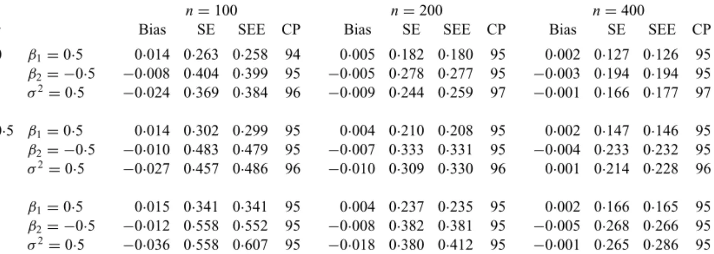
To evaluate the performance of the proposed methods, we conducted two series of simulation studies. The first series pertained to clustered data, the cluster sizes being 1, 2 and 3 with probabil-ities 0·2, 0·7 and 0·1, respectively. We considered model (1) withK =1 and(t)=log(1+0·5t). We generated two independent cluster-level covariates, the first being Ber(0·5) and the second Un(0, 1). We set the corresponding regression parametersβ1andβ2to 0·5 and−0·5, respectively. We adopted the class of logarithmic transformations indexed by parameter r and obtained the random effectbfromN(0,σ2)whereσ2 =0·5. We generated five potential examination times for each subject, with the first being Un(0, 1)and the gap between any two successive examina-tion times being 0·1+Un(0, 1). We assumed that the study ended at time 5, beyond which no examinations occurred. We simulated 10 000 replicates.
Table1summarizes the results on the estimation ofβ =(β1,β2)T andσ2for various values ofnandr, and Fig.1displays the corresponding results for the estimation of(t). The biases for all parameter estimators are small and decrease asnincreases. The variance estimator forβˆ is accurate, and the variance ofσˆ2tends to be overestimated. The confidence intervals for bothβ andσ2have proper coverage probabilities. Additional studies revealed that the variance estimator forσˆ2and the confidence intervals forσ2become more accurate asσ2increases.
Table 1.Parameterestimationresultsforsimulationstudieswithclustereddata
n=100 n=200 n=400
r Bias SE SEE CP Bias SE SEE CP Bias SE SEE CP
0 β1=0·5 0·014 0·263 0·258 94 0·005 0·182 0·180 95 0·002 0·127 0·126 95 β2= −0·5 −0·008 0·404 0·399 95 −0·005 0·278 0·277 95 −0·003 0·194 0·194 95 σ2=0·5 −0·024 0·369 0·384 96 −0·009 0·244 0·259 97 −0·001 0·166 0·177 97
0·5 β1=0·5 0·014 0·302 0·299 95 0·004 0·210 0·208 95 0·002 0·147 0·146 95 β2= −0·5 −0·010 0·483 0·479 95 −0·007 0·333 0·331 95 −0·004 0·233 0·232 95 σ2=0·5 −0·027 0·457 0·486 96 −0·010 0·309 0·330 96 0·001 0·214 0·228 96
1 β1=0·5 0·015 0·341 0·341 95 0·004 0·237 0·235 95 0·002 0·166 0·165 95 β2= −0·5 −0·012 0·558 0·552 95 −0·008 0·382 0·381 95 −0·005 0·268 0·266 95 σ2=0·5 −0·036 0·558 0·607 95 −0·018 0·380 0·412 95 −0·001 0·265 0·286 95
SE, empirical standard error; SEE, mean standard error estimator; CP, empirical coverage percentage of 95% con-fidence interval. Forσ2, Bias and SEE are based on the median instead of the mean, and the confidence interval is
based on the log transformation. Each entry is based on 10 000 replicates.
Cum
ulativ
e hazard
r = 0·0, n = 100
0·0 0·5 1·0
r = 0·0, n = 200 r = 0·0, n = 400
Cum
ulativ
e hazard
r = 0·5, n = 100
0·0 0·5 1·0
r = 0·5, n = 200 r = 0·5, n = 400
Cum
ulativ
e hazard
r = 1·0, n = 100
0·0 0·5 1·0
Cum
ulativ
e hazard
0·0 0·5 1·0
Cum
ulativ
e hazard
0·0 0·5 1·0
Cum
ulativ
e hazard
0·0 0·5 1·0
Cum
ulativ
e hazard
0·0 0·5 1·0
Cum
ulativ
e hazard
0·0 0·5 1·0
Cum
ulativ
e hazard
0·0 0·5 1·0 r = 1·0, n = 200
0 1 2 3 4
Time
0 1 2 3 4
Time
0 1 2 3 4
Time
0 1 2 3 4
Time
0 1 2 3 4
Time
0 1 2 3 4
Time
0 1 2 3 4
Time
0 1 2 3 4
Time
0 1 2 3 4
Time
r = 1·0, n = 400
families indexed byr1andr2. For each subject, we generated covariates and random effects from the same distributions as in the first series of studies. We set the regression parameters for the first event,(β11,β12), to(0·5,−0·5)and those of the second event,(β21,β22), to(0·4, 0·2). We generated examination times for each subject in the same manner as in the first series of studies. The results for the second series of studies are presented in the Supplementary Material. The basic conclusions are the same as those from the first series.
The variance estimation was based on the first-order numerical differentiation with a pertur-bation constant of 5n−1/2. The results are quite stable for perturbation constants betweenn−1/2
and 10n−1/2. We also evaluated variance estimation based on the second-order numerical differ-entiation and found that the resulting variance estimates may be negative whennis small and the perturbation constant is far away from 5n−1/2. The two variance estimation methods produced similar estimates in most cases. We recommend using 5n−1/2 for both the first-order and the second-order numerical differences.
6. AN EXAMPLE
The Atherosclerosis Risk in Communities Study recruited a cohort of 14 751 Caucasian and African-American individuals from four U.S. communities: Forsyth County, North Carolina; Jackson, Mississippi; suburbs of Minneapolis, Minnesota; and Washington County, Mary-land (The ARIC Investigators, 1989). The participants underwent a baseline examination in 1987–1989, three follow-up examinations at approximately three-year intervals, and a further examination in 2011–2013. One important objective of the study was to investigate risk factors for diabetes and hypertension. The definition of diabetes was a fasting glucose level of 126 mg/dL or above, a nonfasting glucose level of 200 mg/dL or above, self-reported physician diagnosis of diabetes, or use of diabetic medication. The definition of hypertension was systolic blood pressure of 140 mmHg or higher, diastolic blood pressure of 90 mmHg or higher, or use of antihypertensive medication. Both events were determined at the examination times and thus interval-censored.
We related the incidence of diabetes and hypertension to race, gender, communities and five baseline risk factors: age, body mass index, glucose level, systolic blood pressure and diastolic blood pressure. We excluded 5890 individuals with prevalent diabetes or hypertension and 124 individuals with unknown status at baseline. After removing another two individuals with missing values of baseline risk factors, we were left with a total of 8735 individuals. We fitted model (1) withK =2,J =1 andb∼N(0,σ2).
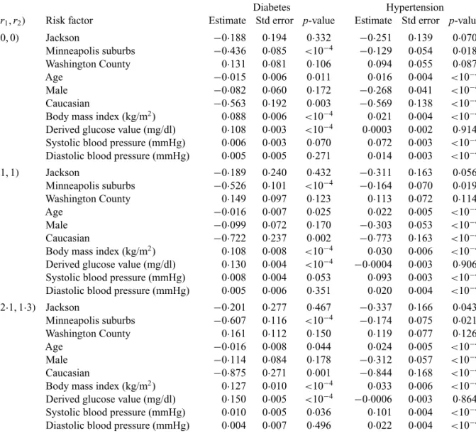
The loglikelihood is maximized at r1 = 2·1 and r2 = 1·3, which is the combination that would be selected by the Akaike information criterion. The loglikelihood values are−12 492·67, −12 412·67 and−12 403·46 at(r1,r2)=(0, 0),(1, 1)and(2·1, 1·3), respectively.
Table 2 shows regression analysis results for the aforementioned three combinations of r1 and r2. The p-values are similar. The results indicate that African-Americans are more likely to develop diabetes and hypertension than Caucasians; baseline body mass index is positively associated with the risk of both diabetes and hypertension; and baseline glucose level is positively associated with the risk of diabetes but not hypertension. Not surprisingly, baseline systolic and diastolic blood pressures are positively associated with the risk of hypertension. Becausen is large, some of thep-values are extremely small.
Table2.RegressionanalysisresultsfortheAtherosclerosisRiskinCommunitiesStudy
Diabetes Hypertension
(r1,r2) Risk factor Estimate Std error p-value Estimate Std error p-value (0, 0) Jackson −0·188 0·194 0·332 −0·251 0·139 0·070
Minneapolis suburbs −0·436 0·085 <10−4 −0·129 0·054 0·018
Washington County 0·131 0·081 0·106 0·094 0·055 0·087 Age −0·015 0·006 0·011 0·016 0·004 <10−4
Male −0·082 0·060 0·172 −0·268 0·041 <10−4
Caucasian −0·563 0·192 0·003 −0·569 0·138 <10−4
Body mass index (kg/m2) 0·088 0·006 <10−4 0·021 0·004 <10−4
Derived glucose value (mg/dl) 0·108 0·003 <10−4 0·0003 0·002 0·914
Systolic blood pressure (mmHg) 0·006 0·003 0·070 0·072 0·003 <10−4
Diastolic blood pressure (mmHg) 0·005 0·005 0·271 0·014 0·003 <10−4 (1, 1) Jackson −0·189 0·240 0·432 −0·311 0·163 0·056
Minneapolis suburbs −0·526 0·101 <10−4 −0·164 0·070 0·019
Washington County 0·149 0·097 0·123 0·113 0·072 0·114 Age −0·016 0·007 0·025 0·022 0·005 <10−4
Male −0·099 0·072 0·170 −0·303 0·053 <10−4
Caucasian −0·722 0·237 0·002 −0·773 0·163 <10−4
Body mass index (kg/m2) 0·108 0·008 <10−4 0·030 0·006 <10−4
Derived glucose value (mg/dl) 0·130 0·004 <10−4 −0·0004 0·003 0·906
Systolic blood pressure (mmHg) 0·008 0·004 0·053 0·093 0·003 <10−4
Diastolic blood pressure (mmHg) 0·005 0·006 0·351 0·020 0·004 <10−4 (2·1, 1·3) Jackson −0·201 0·277 0·467 −0·337 0·166 0·043
Minneapolis suburbs −0·607 0·116 <10−4 −0·174 0·075 0·021
Washington County 0·161 0·112 0·150 0·119 0·077 0·126 Age −0·016 0·008 0·044 0·024 0·005 <10−4
Male −0·114 0·084 0·178 −0·312 0·057 <10−4
Caucasian −0·875 0·271 0·001 −0·844 0·168 <10−4
Body mass index (kg/m2) 0·127 0·010 <10−4 0·033 0·006 <10−4
Derived glucose value (mg/dl) 0·150 0·005 <10−4 −0·0006 0·003 0·864
Systolic blood pressure (mmHg) 0·010 0·005 0·036 0·101 0·004 <10−4
Diastolic blood pressure (mmHg) 0·004 0·007 0·496 0·022 0·004 <10−4
proportional hazards model. The variance component σ2 was estimated at 0·591, 0·646 and 0·758 under the proportional hazards, proportional odds and selected models, respectively, and the corresponding standard error estimates were 0·057, 0·087 and 0·111. Thus, there is strong evidence for dependence of diabetes and hypertension.
Figure2shows the prediction of development of diabetes and hypertension for a Caucasian female and an African-American female with all other risk factors equal. The risk of both diseases is considerably higher for the African-American individual than the Caucasian individual. The three models yield appreciably different estimates of disease-free probabilities.
7. REMARKS
0 5 10 15 20 25 0 5 10 15 20 25
0·0 0·2 0·4 0·6 0·8 1·0
Follow-up time (years)
Disease-free probabilities
0.0 0·2 0·4 0·6 0·8 1·0
(b) (a)
Follow-up time (years)
Disease-free probabilities
Fig. 2. Estimation of disease-free probabilities for an African-American female and a Caucasian female residing in Forsyth County, North Carolina, of age 53 years, with a body mass index of 30 kg/m2, glucose level of 97 mg/dl, systolic
blood pressure of 125 mmHg and diastolic blood pressure of 70 mmHg: (a) diabetes; (b) hypertension. In each panel the upper solid, dashed and dotted curves represent the Caucasian individual under the proportional hazards, proportional odds and selected models, respectively; the lower solid, dashed and dotted curves pertain to the African-American
individual under the proportional hazards, proportional odds and selected models, respectively.
presented in this paper, the convergence criterion was that the maximal relative change in the parameter estimates at two successive iterations should be less than 0·0005. With this criterion, it took less than half a second to analyse one simulated dataset with n = 200. It took about 10 hours to analyse the Atherosclerosis Risk in Communities Study data, which involves 8765 subjects with 10 covariates and 2240 or 2303 distinct interval endpoints for diabetes or hyper-tension, respectively; the computing time was shortened to about one hour when the distinct values were reduced to 133 for diabetes and 138 for hypertension by rounding the examination times to the nearest month. The software implementing the proposed methods is available at http://dlin.web.unc.edu/software.
We have assumed that the support of the examination times for the kth type of event is an interval [0,τk]. We can relax this assumption to let the support consist of intervals or a finite number of discrete time-points. The asymptotic results continue to hold, although the consistency for ˆk in Theorem 1 should be stated to hold in the support of the examina-tion times. In the proofs, the integraexamina-tion over [0,τk]should be changed to integration over the support.
The framework presented in this paper can be extended to other types of multivariate data. In particular, model (1) can be extended to panel count data (Zhang, 2002) by treating as the intensity function of a counting process rather than the hazard function of a failure time. In addition, model (1) can be combined with a generalized linear mixed model that shares the random effects to jointly model longitudinal and survival data (Henderson et al.,2000;Zeng & Lin,2007). There are new theoretical and computational challenges in estimating such multivariate models with interval-censored data.
ACKNOWLEDGEMENT
Risk in Communities Study was carried out as a collaborative study supported by the National Heart, Lung, and Blood Institute. The authors thank the staff and participants of the ARIC study for their important contributions.
SUPPLEMENTARY MATERIAL
Supplementary material available atBiometrikaonline includes three lemmas as well as three figures and six tables presenting additional simulation results.
APPENDIX
Proofs of the asymptotic results
In this appendix we prove Theorems1–3. The proofs make use of three lemmas, which are stated and proved in the Supplementary Material. It is convenient to use empirical process notation:Pndenotes the
empirical measure fornindependent clusters,Pis the true probability measure, andGn=n1/2(Pn−P)is
the empirical process. LetL(θ,A)be the likelihood for a single cluster, such that the loglikelihood is
l(θ,A)=log
"J
j=1 K
k=1
Djk(Ujk,b;β,k)
#
φ(b;)db
where Djk(Ujk,b;β,k) =
Mjk
l=0jkl{Qjk(Ujkl,b;β,k) − Qjk(Ujk,l+1,b;β,k)}, Ujk = (Ujk1,
. . .,Ujk,Mjk)andjkl=I(UjklTjk <Ujk,l+1).
Proof of Theorem1. We first show that lim supnˆk(τk−) <∞with probability 1 for any >0 and
k∈ {1,. . .,K}. Write
m(θ,A)=log
L(θ,A)+L(θ0,A0)
2 ,
whereA0=(01,. . .,0K). Since(θˆ,Aˆ)maximizes the likelihood,
Pnl(θˆ,Aˆ)Pnl(θ0,A0)=Pnm(θ0,A0).
We show in Lemma 1 thatM= {m(θ,A):θ ∈,A∈L}is a Glivenko–Cantelli class, whereLis the set ofK-dimensional nondecreasing functions(1,. . .,K)withk(0)=0. Hence,(Pn−P)m(θ0,A0)
converges to zero almost surely. With probability one,
lim inf
n Pnl(θˆ,
ˆ
A)lim inf
LetM˜ =sup1kKsupt∈[0,τk]{supXjk,β|β T
Xjk(t)|+supZjk|Zjk(t)|}, which is finite under Conditions1–3. For
any >0,
lim inf
n Pnl(
ˆ
θ,Aˆ)
lim sup
n P
n
" log
$ J
j=1 K
k=1
exp
−Gk
UjkMjk
0
exp{ ˆβT
Xjk(s)+bTZjk(s)}dˆk(s)
jkMjk
×φ{b;(γ )ˆ }db %# lim sup n Pn log
" J
j=1 K
k=1
&
exp'−Gk
exp(− ˜M− ˜Mb)ˆk(UjkMjk)
()jkMjk
×φ{b;(γ )ˆ }db #! lim sup n Pn log "
b1 J
j=1 K
k=1
&
exp'−Gk
exp(−2M˜)ˆk(UjkMjk)
()jkMjk
φ{b;(γ )ˆ }db #!
+lim sup
n P
n
log
b>1
φ{b;(γ )ˆ }db
−lim sup
n Pn
J
j=1 K
k=1
jkMjkGk
exp(−2M˜)ˆk(UjkMjk)
!
−lim sup
n P
n
J
j=1 K
k=1
jkMjkI(UjkMjk τk−)Gk
exp(−2M˜)ˆk(τk−)
! . Thus, lim sup n P n J
j=1 K
k=1
jkMjkI(UjkMjk τk−)Gk
exp(−2M˜)ˆk(τk−)
!
=O(1)
for any >0. Since
Pn
" J
j=1
jkMjkI(UjkMjk τk−)
#
→E " J
j=1
jkMjkI(UjkMjk τk−)
# ,
which is positive under Condition5, lim supnGk{exp(−2M˜)ˆk(τk−)}<∞. If lim supnˆk(τk−)= ∞,
thenGk{exp(−2M˜)ˆk(τk−)} = ∞under Condition6. This is a contradiction. Therefore lim supnˆk(τk− ) <∞with probability 1 for any >0 and anyk∈ {1,. . .,K}.
For anyk=1,. . .,K, consider an increasing sequence{τks}(s=1, 2,. . . )such that lims→∞τks=τk.
For any given subsequence ofˆk, Helly’s selection theorem, together with the fact thatˆk(τks) < ∞,
allows us at stagesto choose from the subsequence selected at stages−1 a further subsequence which converges weakly on[0,τks]. We form a final subsequence, still denoted by{ ˆk}, whosesth element is
thesth element of the sequence selected at stages. It is clear thatˆkconverges weakly to some function,
say∗k, in any compact subset of[0,τk). Since the Lebesgue measure for the pointτk is zero,ˆk →∗k
converge to∗k(t)}is zero. Sinceβˆandγˆ are bounded, by choosing a further subsequence, which we still
denote by(ˆ1,. . .,ˆK,βˆ,γ )ˆ , we can assume thatˆk converges to∗k almost everywhere and that(βˆ,γ )ˆ
converges to some constant(β∗,γ∗).
Write θ∗ = (β∗,γ∗)andA∗ = (∗1,. . .,∗K). We wish to show that (θ∗,A∗) = (θ0,A0). By the
concavity of the log function,
Pnm(θˆ,Aˆ)
1 2
PnlogL(θˆ,Aˆ)+PnlogL(θ0,A0)
Pnm(θ0,A0).
Thus(Pn−P)m(θˆ,Aˆ)+Pm(θˆ,Aˆ) (Pn−P)m(θ0,A0)+Pm(θ0,A0). Sincem(θˆ,Aˆ) ∈ M, (Pn−
P)m(θˆ,Aˆ)→0 almost surely. Also, since|*Jj=1*Kk=1Djk(Ujk,b;β,k)|<1 for anyβ ∈BandA∈L
with probability 1, we see that with respect to the probability measure forUjk(j=1,. . .,J;k=1,. . .,K),
J
j=1 K
k=1
Djk(Ujk,b;βˆ,ˆk)− J
j=1 K
k=1
Djk(Ujk,b;β∗,∗k)→0.
By the dominated convergence theorem,
Pm(θˆ,Aˆ)−Pm(θ∗,A∗)
Pm(θˆ,Aˆ)−Pm(βˆ,γ∗,)ˆ + Pm(βˆ,γ∗,)ˆ −Pm(θ∗,A∗)
=O(1) ˆγ−γ∗ +Plog
*J
j=1
*K
k=1Djk(Ujk,b;βˆ,ˆk)
φ{b;(γ∗)}db+L(θ0,A0)
*J
j=1
*K
k=1Djk(Ujk,b;β∗,∗k)
φ{b;(γ∗)}db+L(θ0,A0)
.
Hence|Pm(θˆ,Aˆ)−Pm(θ∗,A∗)| →0 almost surely, such that
PlogL(θ
∗,A∗)+L(θ
0,A0)
2 Pl(θ0,A0).
By the properties of the Kullback–Leibler information,L(θ0,A0)=L(θ∗,A∗)with probability 1. So
"J
j=1 K
k=1
Djk(Ujk,b;β∗,∗k)
#
φ{b;(γ∗)}db=
"J
j=1 K
k=1
Djk(Ujk,b;β0,0k)
#
φ{b;(γ0)}db
with probability 1. For anyj ∈ {1,. . .,J},k ∈ {1,. . .,K}andljk ∈ {0,. . .,Mjk}, we setjkl =1 in the
above equation forl=ljk,. . .,Mjkand take the sum of the resulting equations to obtain
Qjk(Ujkljk,b;β∗,∗k)
⎧ ⎨ ⎩
J
j=1,j|=j K
k=1,k|=k
Djk(Ujk,b;β∗,∗k)
⎫ ⎬
⎭φ{b;(γ∗)}db
=
Qjk(Ujkljk,b;β0,0k)
⎧ ⎨ ⎩
J
j=1,j|=j K
k=1,k|=k
Djk(Ujk,b;β0,0k)
⎫ ⎬
This equality holds for arbitraryljk. Therefore, for anytjk ∈ [0,τk],
Qjk(tjk,b;β∗,∗k)
⎧ ⎨ ⎩
J
j=1,j|=j K
k=1,k|=k
Djk(Ujk,b;β∗,∗k)
⎫ ⎬
⎭φ{b;(γ∗)}db
=
Qjk(tjk,b;β0,0k)
⎧ ⎨ ⎩
J
j=1,j|=j K
k=1,k|=k
Djk(Ujk,b;β0,0k)
⎫ ⎬
⎭φ{b;(γ0)}db.
For some fixedj ∈ {1,. . .,J}andk ∈ {1,. . .,K}, we repeat this process for(j,k)∈ Cjk = {1,. . .,j} ×
{1,. . .,k}to obtain
⎡ ⎣ ⎧ ⎨ ⎩ j
j=1 k
k=1
Qjk(tjk,b;β∗,∗k)
⎫ ⎬ ⎭ ⎧ ⎨ ⎩
(j,k)/∈Cjk
Djk(Ujk,b;β∗,∗k)
⎫ ⎬ ⎭ ⎤
⎦φ{b;(γ∗)}db
= ⎡ ⎣ ⎧ ⎨ ⎩ j
j=1 k
k=1
Qjk(tjk,b;β0,0k)
⎫ ⎬ ⎭ ⎧ ⎨ ⎩
(j,k)/∈Cjk
Djk(Ujk,b;β0,0k)
⎫ ⎬ ⎭ ⎤
⎦φ{b;(γ0)}db.
Settingjkl =1 in the above equation for(j,k) /∈Cjkandl =0,. . .,Mjk and then taking the sum of
the resulting equations gives
⎧⎨
⎩
j
j=1 k
k=1
Qjk(tjk,b;β∗,∗k)
⎫ ⎬
⎭φ{b;(γ∗)}db=
⎧⎨
⎩
j
j=1 k
k=1
Qjk(tjk,b;β0,0k)
⎫ ⎬
⎭φ{b;(γ0)}db.
By Condition7,β∗=β0,γ∗=γ0and∗k(t)=0k(t)fork ∈ {1,. . .,K}andt∈ [0,τk]. Since0k(t)is
continuous, ˆθ−θ0 +
K
k=1supt∈[0,τk]| ˆk(t)−0k(t)| →0 almost surely.
Proof of Theorem2. LetHjkl(t;θ,A)denote
Bjk(t,Ujkl,Ujk,l+1,b;β,k)
*J
j=1,j|=j
*K
k=1,k|=kDjk(Ujk,b;β,k)
φ{b;(γ )}db
*J
j=1
*K
k=1Djk(Ujk,b;β,k)
φ{b;(γ )}db ,
where
Bjk(t,u,v,b;β,k)=exp{βTXjk(t)+bTZjk(t)}
×
Qjk(v,b;β,k)Gk
v
0
exp{βT
Xjk(s)+bTZjk(s)}dk(s)
I(vt)
−Qjk(u,b;β,k)Gk
u
0
exp{βT
Xjk(s)+bTZjk(s)}dk(s)
I(ut)
.
For a single cluster, the score function forθis
lθ(θ,A)=
lβ(θ,A) lγ(θ,A)
where
lβ(θ,A)=
J
j=1 K
k=0 Mjk
l=0
jkl
τk
0
Hjkl(t;θ,A)Xjk(t)dk(t),
lγ(θ,A)=
*J
j=1
*K
k=1Djk(Ujk,b;β,k)
φ
γ{b;(γ )}db
*J
j=1
*K
k=1Djk(Ujk,b;β,k)
φ{b;(γ )}db.
To obtain the score operator forA, we consider a one-dimensional submodelA(h)whereh=(h1,. . .,hK)T
is a vector of functions inL2[0,τk]. Specifically, the submodel specifies that dk,,hk =(1+hk)dk. The
score function forAalong this submodel is
lA(θ,A)(h)=
J
j=1 K
k=1 Mjk
l=0
jkl
τk
0
Hjkl(t;θ,A)hk(t)dk(t).
Clearly,
Gn{lθ(θˆ,Aˆ)} = −n1/2'P{lθ(θˆ,Aˆ)} −P{lθ(θ0,A0)}
( ,
Gn{lA(θˆ,Aˆ)}(h)= −n1/2
'
P{lA(θˆ,Aˆ)(h)} −P{lA(θ0,A0)(h)}
( .
We apply Taylor series expansion at(θ0,A0)to the right-hand sides of the above two equations. In light of
Lemma 3, the second-order terms are bounded by
n1/2E
O(1)
J
j=1 K
k=1 Mjk
l=0
ˆ
k(Ujkl)−0k(Ujkl)
2
+O(1) ˆβ−β02+O(1) ˆγ−γ02
=n1/2Op(n−2/3)+Op
+
ˆβ−β02+ ˆγ−γ02
,
=Op
+
n1/2 ˆβ−β02+n1/2 ˆγ−γ02+n−1/6
, .
Therefore
Gn{lθ(θˆ,Aˆ)} = −n1/2
'
P{lθθ(θˆ−θ0)+lθA(Aˆ−A0)}
(
+Op
+
n1/2 ˆβ−β02+n1/2 ˆγ−γ02+n−1/6
, ,
Gn{lA(θˆ,Aˆ)(h)} = −n1/2
'
P{lAθ(h)(θˆ−θ0)+lAA(h,Aˆ−A0)}
(
+Op
+
n1/2 ˆβ−β02+n1/2 ˆγ−γ02+n−1/6
, ,
wherelθθ is the second derivative of l(θ,A)with respect to θ,lθA(h)is the derivative of lθ along the submodel dA,h,lAθ(h)is the derivative oflA(h)with respect toθ, andlAA(h,Aˆ−A0)is the derivative of lA(h)along the submodel dA0+d(Aˆ−A0). All the derivatives are evaluated at(θ0,A0).
Leth∗denote the least favourable direction such that
l∗AlA(h∗)=lA∗lθ, (A1)
wherel∗Ais the adjoint operator oflA. Note thath∗is a{p+d(d+1)/2}-dimensional vector of functions
follows that
E{lAA(h∗,Aˆ−A0)} = −E{lA(h∗)lA(Aˆ−A0)} = −
lA∗lA(h∗)d(Aˆ−A0)
= −
lA∗lθd(Aˆ−A0)=E{lθA(Aˆ−A0)},
so that
Gn{lθ(θˆ,Aˆ)−lA(θˆ,Aˆ)(h∗)} =n1/2E
'
{lθ−lA(h∗)}⊗2((θˆ−θ0)
+Op
+
n1/2 ˆβ−β02+n1/2 ˆγ−γ02+n−1/6
, .
In addition, if we can show thatlθ(θˆ,Aˆ)−lA(θˆ,Aˆ)(h∗)belongs to a Donsker class and that the matrix E[{lθ−lA(h∗)}⊗2]is invertible, thenn1/2(θˆ−θ
0)=Op(1)and
n1/2(θˆ−θ0)=(E[{lθ −lA(h∗)}⊗2])−1Gn{lθ −lA(h∗)} +op(1).
The influence function forθˆis the efficient influence function, such thatn1/2(θˆ−θ0)converges weakly to
a zero-mean normal random vector whose covariance matrix attains the semiparametric efficiency bound. It remains to show the existence ofh∗, the Donsker property oflθ(θˆ,Aˆ)−lA(θˆ,Aˆ)(h∗), and the non-singularity of the matrixE[{lθ−lA(h∗)}⊗2]. To show that there exists a solutionh∗to (A1), we equipH with an inner product defined by
h(1),h(2) =
K
k=1
τk
0
h(1)k (t)h(2)k (t)d0k(t).
For anyh(1),h(2)∈H,
PlA(h(1))lA(h(2))=
K
k=1
τk
0
k(h(1))(t)h( 2)
k (t)d0k(t),
where
k(h)(t)= K
k=1
τ
k
0 J
j=1 E
⎡ ⎣ ⎧ ⎨ ⎩
Mjk
l=0
jklHjkl(s;θ0,A0)
⎫ ⎬ ⎭
×
⎧ ⎨ ⎩
J
j=1 Mjk
l=0
jklHjkl(t;θ0,A0)
⎫ ⎬ ⎭ ⎤
⎦hk(s)d0k(s).
We define a seminormh = (h),h1/2 on the spaceH. Ifh = 0 for someh ∈ H, then 0 =
(h),h =P{lA(h)2}. Therefore, with probability 1, lA(h)=0, i.e.,
J
j=1 K
k=1
⎡ ⎣ ⎧ ⎨ ⎩
J
j=1,j|=j K
k=1,k|=k
Djk(Ujk,b;β0,0k)
⎫ ⎬ ⎭
×
Mjk
l=0
jkl
τk
0
Bjk(t,Ujkl,Ujk,l+1,b;β0,0k)hk(t)d0k(t)
⎤
By the arguments in the proof of Lemma 3,hk(t)=0 for anyk=1,. . .,K andt ∈ [0,τk]. So · is a
norm inH. Clearly,h chfor some constantc. By the bounded inverse theorem in Banach space,
h chfor some constantc. By the Lax–Milgram theorem (Zeidler,1995), there exists a solution
to (A1). Differentiation of this integral equation with respect totyields
g1k(t)h∗k(t)+ K
k=1
τk
t
g2k(s,t)h∗k(s)ds+
t
0
g3k(s,t)h∗k(s)ds =g4k(t),
where g1k(t) > 0 and thegjk (j = 1, 2, 3, 4)are continuously differentiable functions. Thus, h∗k(·)is
continuously differentiable in [0,τk] for k ∈ {1,. . .,K}. By the arguments in the proof of Lemma 2,
lθ(θˆ,Aˆ)−lA(θˆ,Aˆ)(h∗)belongs to a Donsker class and converges inL2(P)-norm tolθ −lA(h∗).
Finally, we verify thatE[{lθ−lA(h∗)}⊗2]is invertible. If the matrix is singular, then there exist vectors v =(v1,v2)withv1 ∈ Rpandv2 ∈ Rd(d+1)/2 such thatvTE[{lθ −lA(h∗)}⊗2]v =0. It follows that, with
probability 1, the score function along the submodel{θ0+v,A(vTh∗)}is zero. That is,
J
j=1 K
k=1
⎧ ⎨ ⎩
J
j=1,j|=j K
k=1,k|=k
Djk(Ujk,b;β0,0k)
⎫ ⎬ ⎭
Mjk
l=0
jkl
τk
0
Bjk(t,Ujkl,Ujk,l+1,b;β0,0k)
× {vT
1Xjk(t)−vTh∗(t)}d0k(t)φ(b;0)db−
"J
j=1 K
k=1
Djk(Ujk,b;β0,0k)
# vT
2φγ(b;0)db=0
with probability 1. For anyj ∈ {1,. . .,J},k ∈ {1,. . .,K}andljk ∈ {0,. . .,Mjk}(j = 1,. . .,j;k =
1,. . .,k), we evaluate the above equation at all possible values ofjklwith(j,k)∈Cjk = {1,. . .,j} ×
{1,. . .,k}andl=ljk,. . .,Mjkand take the sum of the resulting equations. We then consider all possible
values ofjkl with(j,k) /∈ Cjk andl =0,. . .,Mjk and take the sum of the resulting equations. This
yields
⎧⎨
⎩
j
j=1 k
k=1
Qjk(Ujkljk,b;β0,0k)
⎫ ⎬ ⎭ × j
j=1 k
k=1 Gk
Ujkljk
0
exp{βT
0Xjk(t)+bTZjk(t)}d0k(t)
×
Ujkljk
0
exp{βT
0Xjk(t)+bTZjk(t)}{vT1Xjk(t)−vTh∗k(t)}d0k(t)φ(b;0)db
−
⎧⎨
⎩
j
j=1 k
k=1
Qjk(Ujkljk,b;β0,0k)
⎫ ⎬
⎭v2Tφγ(b;0)db=0.
This equality holds for anyUjkljk. Hence, for anytjk ∈ [0,τk](j
=1,. . .,j; k=1,. . .,k),
⎧⎨
⎩
j
j=1 k
k=1
Qjk(tjk,b;β0,0k)
⎫ ⎬ ⎭ ⎛
⎝j
j=1 k
k=1 Gk
tjk
0
exp{βT
0Xjk(t)+bTZjk(t)}d0k(t)
×
tjk
0
exp{βT
0Xjk(t)+bTZjk(t)}{vT1Xjk(t)−vTh∗k(t)}d0k(t)−
vT
2φγ(b;0)
φ(b;0)
⎞ ⎠