DEVELOPING MACHINE LEARNING METHODOLOGY FOR PRECISION HEALTH
Xiaotong Jiang
A dissertation submitted to the faculty of the University of North Carolina at Chapel Hill in partial fulfillment of the requirements for the degree of Doctor of Philosophy in the Department
of Biostatistics in the Gillings School of Global Public Health.
Chapel Hill 2020
ABSTRACT
Xiaotong Jiang: Developing Machine Learning Methodology for Precision Health (Under the direction of Michael R. Kosorok)
Precision health has been an increasingly popular solution to improve health care quality and guide the decision making process. This includes precision medicine (at the individual level) and precision public health (at the population level such as communities and institutions). By learning from the available medical data with advanced analytical tools, precision health recommends the treatments that are individualized to each patient or entity to maximize clinical outcomes for each individual.
ACKNOWLEDGEMENTS
I dedicate this entire work to my academic and dissertation advisor Michael Kosorok. Dr. Kosorok, I always remember what you told me about how I should take on new tasks that would make me a little bit nervous because that’s the level of challenge that would keep me learning and growing. You are my research mentor and my life mentor who have given me so much support and confidence than anyone else. I am forever grateful to be your student. I acknowledge the following contributors to this research: Chapter 1 collaborators (Richard Loeser, Amanda Nelson, Rebecca Cleveland, Daniel Beavers, Todd Schwartz, Liubov Arbeeva, Carolina Alvarez, Leigh Callahan, and Stephen Messier), Chapter 2 collaborators (Xin Zhou and Kinh Truong), Chapter 3 collaborators (William Stoudemire, Marianne Muhlebach, Lisa Saiman, and Juyan Zhou), NACC research scientists (Jessica Culhane and Merilee Teylan), my dissertation committee members (Donglin Zeng and Jianwen Cai), and all previous and current members of the Kosorok Lab (especially Sebastian Hidalgo, Jingxiang “Sean” Chen, Jon Hibbard, Daniel Luckett, Michael Lawson, Crystal Nguyen, Owen Leete, Xinyi Li, Arkopal Choudhury, Hunyong Cho, and Teeranan “Ben” Pokaprakarn, Nikki Freeman, and John Sperger). You all helped me in many ways and I thank you for your wisdom, financial and moral support. In addition, I acknowledge other close relationships I made at UNC, NCSU, and the Triangle Curling Club (including but not limited to Richard Zink, Busola Sanusi, Laura Zhou, Sean McCabe, Pedro Baldoni, Shaina Mitchell, Jipcy Amador, Eric Van Buren, Scott Van Buren, Anqi Zhu, Jon Rosen, Jiawei Xu, Yue Wang, Ting Wang, Xingjian Yu, Alex Karsten, Antonio LoPiano, Betsy Seagroves, and Melissa Hopgood). These are people who laughed with me, sighed with me, gave me a thumbs up, and gave me a pat on the back during all the ups and downs of graduate school. Our relationships meant a lot to me and made Chapel Hill my second home. Last but not least, to my parents, the continuous help I received from you was tremendous and I am grateful for your selfless support through my toughest and most glorious times in the past six years. I hope I have made you proud.
TABLE OF CONTENTS
LIST OF TABLES . . . ix
LIST OF FIGURES . . . xii
LIST OF ABBREVIATIONS . . . xiv
CHAPTER 1: INTRODUCTION . . . 1
CHAPTER 2: A PRECISION MEDICINE APPROACH TO DEVELOP AND IN-TERNALLY VALIDATE OPTIMAL TREATMENTS FOR OVERWEIGHT AND OBESE SENIOR ADULTS WITH KNEE OSTEOARTHRITIS . . . 3
2.1 Introduction . . . 3
2.2 Patients and Methods . . . 5
2.2.1 Patient Data . . . 5
2.2.2 Preprocessing. . . 5
2.2.3 Training Process and Performance . . . 6
2.2.4 Testing Process and Model Selection . . . 9
2.2.5 Multiple Outcomes . . . 10
2.3 Results. . . 10
2.3.1 The optimal zero-order model (ZOM) . . . 15
2.3.2 The optimal precision medicine model (PMM) . . . 15
2.3.3 The optimal ZOM vs. the optimal PMM . . . 15
2.3.4 Multiple Outcomes . . . 17
2.4 Discussion . . . 18
2.4.1 Limitations . . . 19
2.5.1 Data Cleaning . . . 20
2.5.2 Dimension Reduction . . . 21
2.5.3 Missing Data and Imputation . . . 22
2.5.4 Choice of Models . . . 22
2.5.5 Value Function . . . 25
2.5.6 The Jackknife . . . 25
2.5.7 Model Selection . . . 27
2.5.8 Stratified Cross Validation . . . 27
2.5.9 Multiple Outcomes . . . 29
2.5.10 Generalizability. . . 29
2.6 Simulation Analyses . . . 30
2.6.1 Simulation Settings . . . 30
2.6.2 Simulation Results . . . 33
2.6.3 Consistency of Jackknife Estimators . . . 37
2.6.4 Asymptotic Normality of Jackknife Estimators . . . 38
CHAPTER 3: DEEP DOUBLY ROBUST OUTCOME-WEIGHTED LEARNING . . . 41
3.1 Introduction . . . 41
3.2 Methods . . . 44
3.2.1 Existing Work . . . 44
3.2.2 Deep Doubly Robust Outcome Weighted Learning (DDROWL) . . . 46
3.2.3 Feedforward Neural Networks (FFNN) . . . 47
3.2.4 Deep Kernel Learning (DKL) . . . 48
3.2.5 Theoretical Properties . . . 50
3.2.5.1 Connection to Logistic Regression . . . 50
3.2.5.2 Consistency of Weighted Bootstrap. . . 51
3.3.1 Low-Dimensional Examples . . . 55
3.3.2 High-Dimensional Examples . . . 57
3.4 Application to Medical Data and Imaging. . . 59
3.5 Discussion . . . 67
CHAPTER 4: RISK-ADJUSTED INCIDENCE MODELING ON HIERARCHI-CAL SURVIVAL DATA WITH RECURRENT EVENTS . . . 70
4.1 Introduction . . . 70
4.2 Methods . . . 71
4.2.1 The Frailty Model . . . 71
4.2.2 The Setup and Overview . . . 73
4.2.3 Estimation of Parameters and Their Variability . . . 75
4.2.4 Theoretical Justification . . . 79
4.3 Simulations . . . 81
4.3.1 Simulation Settings . . . 81
4.3.2 Simulation Results . . . 85
4.4 Clinical Implementation . . . 89
4.4.1 Preprocessing. . . 90
4.4.2 Multiple Imputation . . . 91
4.4.3 Survival Model and Variable Selection . . . 92
4.4.4 Results . . . 93
4.5 Discussion . . . 98
CHAPTER 5: FUTURE RESEARCH . . . 100
APPENDIX A: TECHNICAL DETAILS FOR CHAPTER 1. . . 103
APPENDIX B: TECHNICAL DETAILS FOR CHAPTER 2 . . . 107
APPENDIX C: TECHNICAL DETAILS FOR CHAPTER 3 . . . 113
LIST OF TABLES
2.1 Description of input datasets used in the analyses . . . 7 2.2 Listing of precision medicine based machine learning models and
zero-order models used in the analyses . . . 8 2.3 Descriptive characteristics of baseline input datasets . . . 12 2.4 Comparison between the optimal Zero Order Model (ZOM) and the optimal
Precision Medicine Model (PMM) for each outcome . . . 13 2.5 Comparison between the optimal Zero Order Model (ZOM) and the Random
Forrest model for weighted sum of selected outcomes (M6) . . . 14 2.6 Coverage of the empirically true estimatorV0 with 95% CI ofVˆ2based on
100 simulations . . . 35 2.7 Estimated power of jackknifeTsim based on 100 simulations . . . 37 2.8 P-values of Shapiro-Wilk test of normality on jackknifeTsim
0 based on 100 simulations 39
3.9 Listing of constants in DDROWL simulations . . . 54 3.10 Listing of hyperparameters in DDROWL simulations . . . 54 3.11 Mean (sd) of estimated value functions for 5 covariates and 4 simulation
scenarios with sample size800 . . . 56 3.12 Mean (sd) of estimated value functions for 25 covariates and 4 simulation
scenarios with sample size800 . . . 57 3.13 Mean (sd) of estimated value functions for 100 covariates and 4 simulation
scenarios with sample size800 . . . 58 3.14 Mean (sd) of estimated value functions for 800 covariates and 4 simulation
scenarios with sample size800 . . . 58 3.15 Listing of constants and hyperparameters in DDROWL clinical application . . . 65 3.16 Estimated value function of change in cognitive status between initial visit
and the next visit at least a year later and computation time . . . 66 4.17 Simulation constants and parameters . . . 84 4.18 Mean (SD) of estimated covariate coefficients across 100 simulations for
4.19 Mean (SD) of estimated covariate coefficients across 100 simulations for
three time periods based on a mixed effects Cox model. . . 86 4.20 Results of risk-adjusted model of 2012-2014 simulated data validated on
2012-2014 and 2015 simulated data separately, where α is significance level, m is number of blocks in block jackknife estimation of variance, meanCoverage is mean proportion of level-1 groups whose true number of survival cases in the validation set is contained in the risk-adjusted 1−αconfidence interval estimated from the training data averaged across 100 simulations, and AbsCovDiff is absolute difference between the mean
coverage and1−α. . . 87 4.21 Results of risk-adjusted model of 2014 simulated data validated on 2014
and 2015 simulated data separately, where α is significance level, m is number of blocks in block jackknife estimation of variance, meanCoverage is mean proportion of level-1 groups whose true number of survival cases in the validation set is contained in the risk-adjusted 1− α confidence interval estimated from the training data averaged across 100 simulations,
and AbsCovDiff is absolute difference between the mean coverage and1−α. . . 88 4.22 Results of risk-adjusted incidence model of 2014 CFFPR data validated
on 2014 data, where α is significance level, m is number of blocks in block jackknife estimation of variance, Coverage is proportion of programs whose true number of 2014 incidence cases is contained in the risk-adjusted 1−αconfidence interval trained on 2014 data, and AbsCovDiff is absolute
difference between the coverage and1−α.. . . 95 4.23 Results of risk-adjusted incidence model of 2014 CFFPR data validated
on 2015 data, where α is significance level, m is number of blocks in block jackknife estimation of variance, Coverage is proportion of programs whose true number of 2015 incidence cases is contained in the risk-adjusted 1−αconfidence interval trained on 2014 data, and AbsCovDiff is absolute
difference between the coverage and1−α.. . . 96 4.24 Results of risk-adjusted MRSA incidence model of 2012-2014 CFFPR data
validated on 2012-2014 and 2015 data separately, whereαis significance level,mnumber of blocks in block jackknife estimation of variance, Cover-age is proportion of programs whose true number of incidence cases in the test set is contained in the risk-adjusted1−αconfidence interval trained on 2012-2014 data, and AbsCovDiff is absolute difference between the
C.26 Results of risk-adjusted PA incidence model of 2012-2014 CFFPR data validated on 2012-2014 and 2015 data separately, whereαis significance level,mnumber of blocks in block jackknife estimation of variance, Cover-age is proportion of programs whose true number of incidence cases in the test set is contained in the risk-adjusted1−αconfidence interval trained on 2012-2014 data, and AbsCovDiff is absolute difference between the
LIST OF FIGURES
2.1 Flowchart of the proposed precision medicine approach. An asterisk means the step was not performed in this analysis due to unavailable data but is
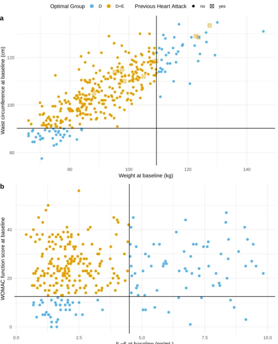
highly recommended for a more complete analysis. . . 11 2.2 Visualization of the estimated optimal decision regimes for outcomes (a)
weight loss since baseline and (b) IL-6 at 18 months. Scatter plots of data for each individual are color-coded to indicate the optimal treatment group assignment of all individuals in the input data (input data 1 for outcome weight loss since baseline in panel (a) and input data 2 for outcome IL-6 at 18 months in panel (b)). Blue indicates individuals who would be assigned to diet only (D) and orange to those assigned to diet plus exercise (D+E). For weight loss since baseline (a), previous heart attack (yes or no) also determined group assignment and is shown as a checked box for those individuals who met that criteria. The horizontal and vertical reference lines indicate the cut-off levels for the variables shown on the horizontal
and vertical axis, respectively, that determined group assignment. . . 16 2.3 True decision boundaries of simulation scenarios (where white, light gray,
and dark gray areas represent true optimal treatment 0, 1, and 2 respectively) . . . 31 2.4 Estimated decision boundaries for a simulated dataset of size n = 500 trained
by KRR models (scenario 1 - circles, scenario 2 - steps, scenario 3 – lines,
scenario 4 – quadratic curves) . . . 34 2.5 Q-Q plots of the distribution of estimatorsVˆ1toVˆ4versus the distribution of
ˆ
V4based on the KRR model across 100 simulations forn= 50andn= 400
over 4 scenarios (empirical is red, jackknife is green, empirical+test is
purple, jackknife+test is blue) . . . 36 2.6 Q-Q plots of the distribution of jackknifeTsim
0 versus the standard normal
distribution across 100 simulations forn= 50andn = 400over4scenarios . . . 40 3.7 Diagram of the DDROWL architecture for the NACC data application . . . 64 4.8 Diagram of the risk-adjusted survival analysis (from left to right). Steps
marked with asterisks are optional but recommended if applicable. . . 74 4.9 Histograms of estimated versus observed (true) number of survival events
for different training and validation periods cumulative across 100 simu-lations (top left: 2012-2014 training and validation, topright 2012-2014 training and 2015 validation, bottom left: 2014 training and validation,
4.10 Histogram of estimated versus observed (true) number of 2014 MRSA and
PA incidence cases where the risk-adjusted model is trained from 2014 data . . . 95 4.11 Histogram of estimated versus observed (true) number of 2015 MRSA and
PA incidence cases where the risk-adjusted model is trained from 2014 data . . . 97 C.12 Histogram of estimated versus observed (true) number of 2012-2014 (top)
and 2015 (bottom) MRSA and PA incidence cases where the risk-adjusted
LIST OF ABBREVIATIONS AOL Augmented Outcome-weighted Learning
CDF Cumulative Distribution Function
CF Cystic Fibrosis
CFFPR Cystic Fibrosis Foundation Patient Registry CI Confidence Interval
CV Cross Validation
DDROWL Deep Doubly Robust Outcome Weighted Learning DNN Deep Neural Network
DKL Deep Kernel Learning FFNN Feedforward Neural Network IPW Inverse Probability Weighting ITR Individualized Treatment Rule
JK Jackknife
KOA Knee Osteroarthritis
LASSO Least Absolute Shrinkage and Selection Operator
MI Multiple Imputation
MLE Maximum Likelihood Estimation
NACC National Alzheimer’s Coordinating Center OWL Outcome Weighted Learning
PDF Probability Density Function
RF Random Forest
RLT Reinforcement Learning Trees RWL Residual Weighted Learning SD Standard Deviation
CHAPTER 1: INTRODUCTION
With the rapid developments in science and technology, the sheer amount of data generated in healthcare and health-related research has been both empowering and overwhelming. Machine learning tools are able to absorb more and learn better about health policy and behaviors because they are no longer constrained with homogeneity and small sample sizes. Meanwhile, traditionally well-established methods have been challenged because it is difficult to accommodate for the increasing complexity of data, such as source, structure, size, and type. Assigning the same treatment to everybody is often not effective, and there has been a higher and higher demand for new, more powerful analytical methods to target on the well-being of each individual (rather than a population as a whole) and personalize treatments better without strong domain knowledge. This, however, does not mean that we are negating the traditional treatments; instead, we are looking for the treatments (traditional or innovative) that best fit each patient. It is this “big data” era we are living in that offers such opportunities for this precision medicine concept to thrive and sustain. We aim to develop data-driven and generalizable machine learning approaches with weak or minimal assumptions under the framework of precision medicine. More specifically, we will examine the following three research topics.
value and we show evidence of asymptotic normality through simulations. The usage of jackknife estimators is fully studied in a clinical trial called IDEA for knee osteoarthritis.
The existing machine learning approaches have proven their ability in optimal individualized treatment estimation for small sample sizes of observational studies and clinical trials. There is yet room for collaboration between precision medicine and deep learning, the two increasingly popular areas in public health application. The non-parametric hierarchical architecture in deep learning increases the flexibility of existing learning regimes and expands the influence of precision medicine to large, high-dimensional data. We show how to get the best of both worlds between deep learning and augmented outcome weighted learning, a recent method that thrives on doubly robustness and residuals.
Finally, we arrive at the crossroad of precision medicine and survival analysis, where we are interested in monitoring survival time while taking into account multi-level hierarchical structure and recurrent events in right-censored data. we aim to extend a mixed-effect Andersen-Gill model (also known as a frailty model) with risk adjustment and provide variability estimates of the survival time. This method will be particularly useful for infection prevention and control, where health programs or hospitals want to gain knowledge on their infection rates in advance and be able to take proactive actions.
CHAPTER 2: A PRECISION MEDICINE APPROACH TO DEVELOP AND INTER-NALLY VALIDATE OPTIMAL TREATMENTS FOR OVERWEIGHT AND OBESE
SE-NIOR ADULTS WITH KNEE OSTEOARTHRITIS
2.1 Introduction
Knee osteoarthritis (KOA) is one of the most common forms of arthritis worldwide account-ing for a significant proportion of pain and disability in the adult population (Cross et al., 2014). Known risk factors for KOA include older age (especially 55 years and older), increased body weight, previous joint injury, and genetics (Vina and Kwoh, 2018). Clinical trials in overweight and obese adults with symptomatic KOA have shown weight loss and exercise interventions can improve pain and function, although not all individuals achieve a similar amount of benefit (Messier et al., 2013; Nelson et al., 2014; Messier et al., 2018). Overweight and obese patients with KOA will want to know if they need to diet and exercise or whether exercise or diet alone would be sufficient. Likewise, clinicians still have limited knowledge and will need additional insight into which specific therapies are most likely to benefit particular patients in a given situation. To address these questions, we utilized machine learning tools to develop and inter-nally validate the optimal precision medicine treatment regime from OA clinical trial data and simulations that would maximize expected clinical outcomes.
function called a decision rule which maps individual characteristics to a recommended in-tervention. The decision rules are estimated by machine learning models, which have been recommended to aid clinical decision-making (Jamshidi et al., 2018). Although many decision rules could potentially map patient information to a treatment, an optimal treatment rule (or optimal treatment regime) can be identified that maximizes the expected clinical outcomes of interest, thus serving to provide the optimal treatment recommendation to a patient population of interest (Kosorok and Laber, 2018).
We use the precision medicine approach to develop and internally validate the optimal treatment regimen for making exercise and weight loss recommendations for individuals with symptomatic KOA, utilizing data collected during the Intensive Diet and Exercise for Arthritis (IDEA) trial. The IDEA trial compared 3 interventions over 18 months: 1) E - exercise alone (considered standard of care as a control group), 2) D - diet-induced weight loss with the goal of a 10% reduction in body weight, and 3) D+E - diet plus exercise, in overweight and obese adults with symptomatic radiographic KOA (Messier et al., 2013). IDEA results showed that, compared to exercise alone, participants randomized to D and D+E groups had greater weight loss and greater reductions in interleukin-6 (IL-6) at 18th month. The other primary outcome, knee compressive force, was significantly reduced in the D group but not the D+E group. Self-reported pain and function scores improved more in the D+E group. Not unexpectedly, there was a variable response to each intervention among the study participants and those who lost more weight demonstrated more improvements in function, pain, knee compressive force and IL-6 levels (Messier et al., 2013, 2018), independent of group assignment. We hypothesized that one or more of these variables could be used to determine an optimal treatment regime that would inform which individuals would benefit the most (in terms of specific outcomes) from a given intervention when compared to assigning all individuals to just one of the three interventions.
precision medicine-based machine learning approaches to clinical trial data in KOA; iii) These approaches identified subgroups of patients for whom a precision medicine decision rule would lead to improved outcomes over assignment of all individuals to the combined exercise and weight loss intervention.
2.2 Patients and Methods 2.2.1 Patient Data
IDEA was an assessor-blinded, single-center randomized trial conducted during 2006 - 2011 at Wake Forest University and Wake Forest School of Medicine. Details of the study design and the results for the main outcomes have been previously published (Messier et al., 2009, 2013). In brief, IDEA included 454 individuals with mild or moderate radiographic OA in one or both knees. They were ambulatory, community-dwelling persons aged 55 or older (mean66±6 (SD) years) with a body mass index (BMI) between 27 and 41 (mean33.6±3.7(SD) kg/m2),
a sedentary lifestyle, and pain on most days due to KOA. Measures (76 covariates) relevant to participant demographics, standard sociodemographic factors, physical performance measures, KOA, and its effects on pain and function were collected at baseline with selected outcome measures also obtained at 6 months (not used in this study) and 18 months.
2.2.2 Preprocessing
important as determined by the variable importance measure from random forests (RF) (Breiman, 2001). Selected covariates were then imputed via a non-parametric random forest method called missForest (Stekhoven and Bühlmann, 2011), which does not require assumptions about the data distribution, utilizes out-of-bag imputation error estimates to avoid cross validation (CV), and can be applied to high-dimensional mixed-type data of unequal scales. Lastly, categorical variables were conformed and dichotomized, and all outcomes were transformed such that higher values represented improvements in the outcomes. All baseline covariates were standardized to the standard normal distribution to avoid artifacts from differences in scaling, due to the potential for varying scales to create misleading values of coefficients in models such as penalized regression. Missing data were investigated in the original IDEA study with multiple imputation analysis, which “revealed minimal differences from [the] original intention-to-treat analysis” (Messier et al., 2013). Further details on data cleaning, dimension reduction, and imputation are provided in the Supplemental Materials.
A second analysis used all seven outcomes including the two mechanistic outcomes (knee compressive force and plasma IL-6) at 18 months. This analysis was considered so as not to overlook any potentially valuable information from the two mechanistic outcomes, although they are not patient reported or as easily obtainable in clinical practice as the other outcomes. We cleaned and imputed the second input dataset (Input Data 2, Table 2.1) and applied the same preprocessing procedure as described above. Values for IL-6 at 18 months were log-transformed in the analyses due to right-skewness and exponentiated back to original values during testing and optimal estimation.
2.2.3 Training Process and Performance
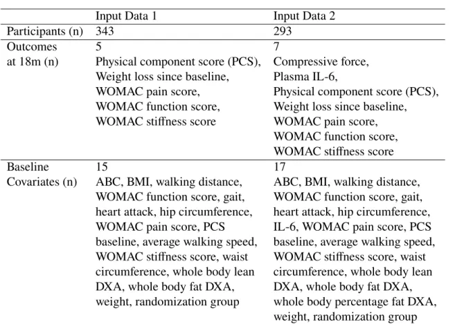
Table 2.1: Description of input datasets used in the analyses
Input Data 1 Input Data 2
Participants (n) 343 293
Outcomes 5 7
at 18m (n) Physical component score (PCS), Compressive force, Weight loss since baseline, Plasma IL-6,
WOMAC pain score, Physical component score (PCS), WOMAC function score, Weight loss since baseline, WOMAC stiffness score WOMAC pain score,
WOMAC function score, WOMAC stiffness score
Baseline 15 17
Covariates (n) ABC, BMI, walking distance, ABC, BMI, walking distance, WOMAC function score, gait, WOMAC function score, gait, heart attack, hip circumference, heart attack, hip circumference, WOMAC pain score, PCS IL-6, WOMAC pain score, PCS baseline, average walking speed, baseline, average walking speed, WOMAC stiffness score, waist WOMAC stiffness score, waist circumference, whole body lean circumference, whole body lean DXA, whole body fat DXA, DXA, whole body fat DXA, weight, randomization group whole body percentage fat DXA,
weight, randomization group
Abbreviations: ABC - Activities-specific balance confidence scale, BMI – Body mass index, DXA – Dual-energy X-ray absorptiometry, IL- Interleukin, PCS – Physical component score, WOMAC - Western Ontario and McMaster Universities OA index
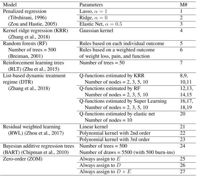
(M21-23), and Bayesian model (M24). Our selection of models covered both conventional and emerging concepts in the statistical literature; the rational for each model choice is included in the Supplemental Materials. In addition to the precision medicine models, we investigated three zero-order models (ZOMs) which assigned just one of the treatments (E, D, D+E) to all participants (M25-27). ZOMs are named after zero-order processes which are fixed decision rules that do not change by individual.
Table 2.2: Listing of precision medicine based machine learning models and zero-order models used in the analyses
Model Parameters M#
Penalized regression Lasso,α= 1 1
(Tibshirani, 1996) Ridge,α= 0 2
(Zou and Hastie, 2005) Elastic Net,α = 0.5 3
Kernel ridge regression (KRR) Gaussian kernel 4
(Zhang et al., 2018)
Random forests (RF) Rules based on each individual outcome 5 Number of trees = 500 Rules based on a weighted outcome 6 (Breiman, 2001) of weight loss, pain, and function
Reinforcement learning trees Number of trees = 50 7
(RLT) (Zhu et al., 2015)
List-based dynamic treatment Q-functions estimated by KRR 8,9,
regime (DTR) Number of nodes = 2, 3, 5, 10 10,11
(Zhang et al., 2018) Q-functions estimated by RF 12,13,
Number of nodes = 2, 3, 5, 10 14,15 Q-functions estimated by Super Learning 16,17,
Number of nodes = 2, 3, 5, 10 18,19 Q-functions estimated by elastic net 20
Number of nodes = 10
Residual weighted learning Linear kernel 21
(RWL) (Zhou et al., 2017) Polynomial kernel with 2nd order 22 Polynomial kernel with 3rd order 23 Bayesian additive regression trees Number of trees = 500 24 (BART) (Chipman et al., 2010) Number of draws = 5500 (with 500 burn-ins)
Zero-order (ZOM) Always assign toE 25
Always assign toD 26
Always assign toD+E 27
the performance and generalization of ITRs on the one remaining fold. This is repeated until every fold has been tested.
We used the jackknife method to estimate the bias and standard error of the estimated value function used for model selection. The jackknife is a a leave-one out cross validation (LOOCV) orn-fold CV method where each individual serves as a fold so the training sample leaves one observation out at a time (Efron and Tibshirani, 1994). We chose the jackknife estimator because it requires weak assumptions (i.e., unrestricted shape of the probability distribution as long as the observations are independently and identically distributed) and is approximately unbiased for the true prediction error (Friedman et al., 2001). In addition, stratified 10-fold CVs were also performed to check the stability of jackknife value function estimates and compare test results. Such validation methods (jackknife and CV) as well as simulation experiments accommodate for internal validation to prevent overfitting. More details on the jackknife and CV estimators as well as simulations on their theoretical properties may be found in subsections: The Jackknife and Stratified Cross Validation in Supplemental Materials.
2.2.4 Testing Process and Model Selection
jackknife validation), which served as the final data-driven, precision medicine-based treatment recommendation.
2.2.5 Multiple Outcomes
To account for potential correlations among outcomes, we derived optimal treatment rules based on a weighted sum across multiple outcomes. A minimax algorithm was proposed to optimize data-driven weights for the three outcomes of greatest interest: weight loss since baseline, WOMAC pain sub score, and WOMAC function sub score at 18 months. To reduce computational time, we used a coarse-to-fine grid search with RF models to determine the weight combination that maximized the lowest jackknife value function estimates among the three outcomes, hence the name “minimax” (details in subsection Multiple Outcomes in Supplemental Materials). The selected minimax weights were then used to create a composite outcome, i.e., the weighted sum of weight loss, pain, and function score, to train a RF model (M6) and estimate the optimal treatment rule. This contrasts with the other models discussed above where the PM treatment rule was trained on a single outcome but all models were tested on a single outcome.
All analyses were performed with R version 3.4.4 (R Core Team, 2019). In formation on specific packages can be found in subsection Choice of Models in Supplementary Materials. As these analyses were exploratory in nature, the significance level was relaxed to be0.1throughout this paper. A complete outline of the entire precision medicine approach is visualized in Figure 2.1.
2.3 Results
Process Input Data (identify outcomes/covariates/treatments, cleaning, feature selection, imputation, etc.)
IdentifycandidateZOMsandPMMs that suit the data
Training and testing all models with internal validation (e.g., jackknife)
Select the optimal ZOM and optimal PMM basedonestimatedvaluefunctions
ComparetheoptimalZOMandoptimalPMM withaZ-test
Output the estimated decision rule of the optimal PMM foroutcomeswithsignifcantresults
Validate the treatment recommendation with external validation*
Figure 2.1: Flowchart of the proposed precision medicine approach. An asterisk means the step was not performed in this analysis due to unavailable data but is highly recommended for a
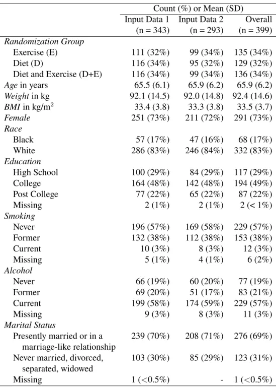
Table 2.3: Descriptive characteristics of baseline input datasets Count (%) or Mean (SD)
Input Data 1 Input Data 2 Overall (n = 343) (n = 293) (n = 399) Randomization Group
Exercise (E) 111 (32%) 99 (34%) 135 (34%)
Diet (D) 116 (34%) 95 (32%) 129 (32%)
Diet and Exercise (D+E) 116 (34%) 99 (34%) 136 (34%)
Agein years 65.5 (6.1) 65.9 (6.2) 65.9 (6.2)
Weightin kg 92.1 (14.5) 92.0 (14.8) 92.4 (14.6)
BMIin kg/m2 33.4 (3.8) 33.3 (3.8) 33.5 (3.7)
Female 251 (73%) 211 (72%) 291 (73%)
Race
Black 57 (17%) 47 (16%) 68 (17%)
White 286 (83%) 246 (84%) 332 (83%)
Education
High School 100 (29%) 84 (29%) 117 (29%)
College 164 (48%) 142 (48%) 194 (49%)
Post College 77 (22%) 65 (22%) 87 (22%)
Missing 2 (1%) 2 (1%) 2 (< 1%)
Smoking
Never 196 (57%) 169 (58%) 229 (57%)
Former 132 (38%) 112 (38%) 153 (38%)
Current 10 (3%) 8 (3%) 12 (3%)
Missing 5 (1%) 4 (1%) 6 (2%)
Alcohol
Never 66 (19%) 60 (20%) 77 (19%)
Former 69 (20%) 51 (17%) 83 (21%)
Current 199 (58%) 174 (59%) 229 (57%)
Missing 9 (3%) 8 (3%) 11 (3%)
Marital Status
Presently married or in a 239 (70%) 208 (71%) 276 (69%) marriage-like relationship
Never married, divorced, 103 (30%) 85 (29%) 123 (31%) separated, widowed
Table 2.4: Com par ison be tw een the op timal Zer o Or der Model (ZOM) and the op timal Pr ecision Medicine Model (PMM) for eac h outcome Dat ase t Outcomes (18 mo.) Op timal Op timal Es timated Relativ e p-ZOM PMM 1 Value Incr ement 2 value 3 (Op timal PMM) In put Ph ysical com ponent scor e D+E M10 45.47 0.10 0.88 Dat a 1 W eight loss since baseline D+E M10 11.21 1.45 0.01 4 (n = 343) W OMA C pain scor e D+E M15 3.25 0.02 0.38 W OMA C function scor e D+E M1, M12 12.63 0.00 1.00 W OMA C stiffness scor e D+E M19 2.12 0.03 0.86 In put Com pr ess for ce D M9 2336.21 21.74 0.73 Dat a 2 Plasma IL -6 D M12 2.29 0.26 0.09 (n = 293) Ph ysical com ponent scor e D+E M7 46.46 0.96 0.24 W eight loss since baseline D+E M7 11.76 1.31 0.06 W OMA C pain scor e D+E M9 3.24 0.08 0.59 W OMA C function scor e D+E M1, M12-15 12.58 0.00 1.00 W OMA C stiffness scor e D+E M8 2.08 0.04 0.31 1 This table focuses on modeling on individual outcomes. PM model selection w as among 23 models in Table 2.2, ex cluding M6 whose results ar e pr esented in Table 2.5. M1-4 ar e penalized reg ression models. M5 and M7 ar e random for es ts and reinf or cement lear ning trees. M8-11, M12-15, and M16-19 ar e respectiv el y ker nel ridg e reg ression, random for es ts, and super lear ning lis t-based D TRs wit h 2, 3, 5, 10 nodes. M20 is elas tic ne tlis t-based D TR wit h 10 nodes. M21-23 ar e residual w eighted lear ning of diff er ent ker nels, and M24 is Ba yesian reg ression model. 2Relativ e incr ement is the jac kknif e es timated value function of the op timal PMM minus the jac kknif e es timated value function of the op timal ZOM; the incr ement in futur e expected outcome based on the op timal PMM relativ e to the op timal
ZOM. 3The
2.3.1 The optimal zero-order model (ZOM)
Considering the three ZOMs, we found that the optimal ZOM model assigned every indi-vidual to D+E for all 5 clinical outcomes: weight loss since baseline, WOMAC pain, function and stiffness scores, and PCS at 18 months (Table 2.4). Treatment D was the optimal ZOM for the two mechanistic outcomes: knee compressive force and plasma IL-6 level at 18 months. 2.3.2 The optimal precision medicine model (PMM)
The RF model with minimax weights (M6) was the optimal PMM for each of the three WOMAC sub scores regardless of input data (Table 2.5). For the rest of the outcomes (Table 2.4), list-based models (M9-13) and RLT (M7) were optimal among the 24 PMMs.
2.3.3 The optimal ZOM vs. the optimal PMM
The relative increments between the estimated value functions of the optimal PMM and those of the optimal ZOM were positive (Table 2.4), indicating that the optimal PMM outperformed the optimal ZOM for all outcomes. According to the Z-test, such improvement of the optimal PMMs compared to the optimal ZOMs was significant both for weight loss since baseline and for IL-6 levels (Table 2.4). We investigated these two outcomes further.
For weight loss between baseline and 18 months, the application of our PM approach showed that future patients are estimated to lose11.2kg of weight on average between baseline and 18 months, according to the optimal PMM (list-based DTR with at most 5 nodes). This is an average of1.4kg more weight loss than if all patients had received D+E, the optimal ZOM (significant improvement, p = 0.01). Trained on input data 1 as a whole, the estimated optimal decision regime for weight loss would recommend intervention D+E to patients who meet either of the following two conditions:
1.1) If, at baseline, weight does not exceed109.35kgandwaist circumference is above90.25 cm,
Optimal Group ● D ● D+E Previous Heart Attack ● no yes ● ● ● ● ● ● ● ● ● ● ● ● ● ● ● ● ● ● ● ● ● ● ● ● ● ● ● ● ● ● ● ● ● ● ● ● ● ● ● ● ● ● ● ● ● ● ● ● ● ● ● ● ● ● ● ● ● ● ● ● ● ● ● ● ● ● ● ● ● ● ● ● ● ●● ● ● ● ● ● ● ● ● ● ● ● ● ● ● ● ● ● ● ● ● ● ● ● ● ● ● ● ● ● ● ● ● ● ● ● ● ● ● ● ● ● ● ● ● ● ● ● ● ● ● ● ● ● ● ● ● ● ● ● ● ● ● ● ● ● ● ● ● ● ● ● ● ● ● ● ● ● ● ● ● ● ● ● ● ● ● ● ● ● ● ● ● ● ● ● ● ● ● ● ● ● ● ● ● ● ● ● ● ● ● ● ● ● ● ● ● ● ● ● ● ● ● ● ● ● ● ● ● ● ● ● ● ● ● ● ● ● ● ● ● ● ● ● ● ● ● ● ● ● ● ● ● ● ● ● ● ● ● ● ● ● ● ● ● ● ● ● ● ● ● ● ● ● ● ● ● ● ● ● ● ● ● ● ● ● ● ● ● ● ● ● ● ● ● ● ● ● ● ● ● ● ● ● ● ● ● ● ● ● ● ● ● ● ● ● ● ● ● ● ● ● ● ● ● ● ● ● ● ● ● ● ● ● ● ● ● ● ● ● ● ● ● ● ● ● ● ● ● ● ● ● ● ● ● ● ● ● ● ● 80 100 120
80 100 120 140
Weight at baseline (kg)
W
aist circumf
erence at baseline (cm)
a ● ● ● ● ● ● ● ● ● ● ● ● ● ● ● ● ● ● ● ● ● ● ● ● ● ● ● ● ● ● ● ● ● ● ● ● ● ● ● ● ● ● ● ● ● ● ● ● ● ● ● ● ● ● ● ● ● ● ● ● ● ● ● ● ● ● ● ● ● ● ● ● ● ● ● ● ● ● ● ● ● ● ● ● ● ● ● ● ● ● ● ● ● ● ● ● ● ● ● ● ● ● ● ● ● ● ● ● ● ● ● ● ● ● ● ● ● ● ● ● ● ● ● ● ● ● ● ● ● ● ● ● ● ● ● ● ● ● ● ● ● ● ● ● ● ● ● ● ● ● ● ● ● ● ● ● ● ● ● ● ● ● ● ● ● ● ● ● ● ● ● ● ● ● ● ● ● ● ● ● ● ● ● ● ● ● ● ● ● ● ● ● ● ● ● ● ● ● ● ● ●● ● ● ● ● ● ● ● ● ● ● ● ● ● ● ● ● ● ● ● ● ● ● ● ● ● ● ● ● ● ● ● ● ● ● ● ● ● ● ● ● ● ● ● ● ● ● ● ● ● ● ● ● ● ● ● ● ● ● ● ● ● ● ● ● ● ● ● ● ● ● ● ● ● ● ● ● ● ● ● ● ● ● ● ● ● ● ● ● ● ● ● 0 20 40
0.0 2.5 5.0 7.5 10.0
IL−6 at baseline (pg/mL)
W
OMA
C function score at baseline
b
Figure 2.2: Visualization of the estimated optimal decision regimes for outcomes (a) weight loss since baseline and (b) IL-6 at 18 months. Scatter plots of data for each individual are color-coded to indicate the optimal treatment group assignment of all individuals in the input
data (input data 1 for outcome weight loss since baseline in panel (a) and input data 2 for outcome IL-6 at 18 months in panel (b)). Blue indicates individuals who would be assigned to
diet only (D) and orange to those assigned to diet plus exercise (D+E). For weight loss since baseline (a), previous heart attack (yes or no) also determined group assignment and is shown as a checked box for those individuals who met that criteria. The horizontal and vertical reference
If neither of these conditions are met, the recommendation is for treatment D. The visualization of this optimal treatment rule can be found in Figure 2.2a.
For IL-6, the application of our PM approach showed that future patients are estimated to decrease IL-6 to2.29pg/mL on average at 18 months, according to the optimal PMM (list-based DTR with at most 2 nodes). This is an average of0.26pg/mL more reduction than if all patients had received D, the optimal ZOM (significant improvement, p = 0.09). Trained on input data 2, the estimated optimal treatment rule for IL-6 assigned D+E to patients who meet the following condition:
2.1) If, at baseline, IL-6 does not exceed4.5pg/mLandWOMAC function score is more than 12.5.
If this condition is not met, patients would be assigned to treatment D (Figure 2.2b). As evidence of stability, we found similar patterns and similar conclusions for weight loss and IL-6 using the stratified 10-fold CV method (see Stratified Cross Validation in Supplementary Materials). 2.3.4 Multiple Outcomes
three WOMAC scores, but not for outcomes uncorrelated to the three weighed outcomes, which are compressive force and IL-6.
2.4 Discussion
In this paper, we investigated optimal treatment recommendations for older and overweight or obese individuals with KOA using precision medicine techniques and machine learning tools applied to data obtained from the IDEA trial. The individual treatment decisions obtained from our precision medicine approach are data-driven (requiring no strong assumptions), reproducible (with careful reporting of the analysis process) (Kosorok and Laber, 2018), and generalizable and extendable to other clinical settings (because of rich heterogeneity in the clinical input data).
The results of the optimal ZOM, where everyone would be assigned to a single intervention, match with those from the published IDEA trial (Messier et al., 2009, 2013). The assignment of patients to the D+E intervention would be expected to result in the optimal improvement in the majority of patients in the clinical outcomes of weight loss since baseline, WOMAC pain, function, and stiffness scores, as well as PCS and so should remain the recommendation of choice. In individuals where the primary goal is to reduce systemic inflammation as measured by plasma IL-6 levels and/or reduce the knee compressive force, D alone would be the treatment of choice.
seen in individuals who have more peripheral adiposity rather than central adiposity. In these cases, D could be more effective in losing weight. The finding that our results were modified by a history of a heart attack may be that the cardiac status of these individuals encourages optimal compliance and improves more with the combined D+E than D alone and this allows for greater activity levels resulting in greater weight loss.
The finding that the IL-6 outcome improves more with D than D+E in certain individuals is not easily explained. We noted that individuals with high baseline IL-6 levels (i.e. above 4.5 pg/mL) or those with low baseline function scores (12.5 or less in a range of 0 to 68) reduced their IL-6 more from diet only. Individuals whose IL-6 was not high but have poorer function are recommended to receive both diet and exercise. The decrease in IL-6 suggests less systemic inflammation but there is no solid evidence to suggest that exercise would modulate the reduction in IL-6 that occurs with dietary weight loss. Because all three groups received an intervention, the significant differences in outcomes noted among the groups at 18 months would be unlikely to be due to regression to the mean. Our findings that specific subgroups of individuals received more benefits from specific interventions argues against the premise that response was simply due to patient perception rather than to the intervention itself.
As for the multiple outcomes, comparison between Table 2.4 and Table 2.5 suggested that our minimax rule together with the coarse-to-fine grid search for parameter optimization can be a useful way to incorporate multiple outcomes, and combining correlated outcomes has the potential for bringing more benefits to patients than single outcomes. However, uncorrelated outcomes do not benefit from the composite outcome.
2.4.1 Limitations
were more interested in the final improvements of each outcome between the start and the end of the trial and less on the intermediate progress. It is also unlikely for adding one more time point shortly after the trial would be influential as we expect it takes time for the interventions to take effect. Thirdly, there were some covariates with a large proportion of missing data excluded from the analysis. The majority of these were measures that would not be routinely collected in the clinical setting such as full-length lower extremity radiographs for alignment, computed tomography for abdominal and thigh fat, knee MRI, and isokinetic strength testing. Finally, our results are from a single clinical trial of patients with mild-to-moderate symptomatic KOA (Kellgren-Lawrence scores of 2-3) (Messier et al., 2013) and may not be generalizable to populations with more severe KOA.
2.5 Supplementary Materials 2.5.1 Data Cleaning
6th and 12th month, kept baseline and 18th month data only, and reshaped the raw data from a long format to a wide format.
2.5.2 Dimension Reduction
2.5.3 Missing Data and Imputation
In addition to the multiple imputation analysis conducted in the original IDEA study, we looked into the missingness pattern in the preprocessed Input Data 2 (with 7 outcomes) from two perspectives. We first performed logistic regression modeling for raw X covariates on the missingness of each outcome (0/1), and none of the X covariates was found to be significant. We also calculated Spearman correlation coefficients between the original data and the corresponding indicator data of 0/1’s (where 0 means the value is not missing, and 1 means it is missing). Mixing the covariates and outcomes together, we randomly sampled five variables at a time (to maintain the size of the square matrix) for the correlation matrix but repeated this random sampling 15 times. Most pairwise correlations between the original data and missingness indicator data were less than 0.2, except around one to six moderate correlations occasionally observed per sample, which was partially due to moderate correlations between the two original variables. After we confirmed that there were no obvious missing data problems, imputation was conducted on covariates missing in less than 15% of the participants because too many missing data points would lead to biases and potentially poorly imputed values. The imputation process was unsupervised (using only X-variables) because more biases would be introduced if outcomes were involved at this stage. The algorithm missForest suit our study because it did not require assumptions about the data distribution, can be applied to high-dimensional mixed-type data of unequal scales, utilized out-of-bag imputation error estimates to avoid CV, and outperformed other popular imputation methods such as multiple imputation by chained equations (MICE) (Stekhoven and Bühlmann, 2011). The R package “missForest” was used to run this imputation (Stekhoven and Bühlmann, 2011).
2.5.4 Choice of Models
of penalty terms (lasso, ridge, and elastic net) that differ in terms of the amount of shrinkage determined by a penalty parameter: lasso (M1) forces coefficients to be exactly zero with an absolute value penalty and ridge (M2) forces the coefficients to be close to zero with a squared term penalty, whereas elastic net (M3) with parameter is an even mix of lasso and ridge. Kernel ridge regression (KRR) (M4) is a ridge regression method that directly computes kernel functions to make predictions and the Gaussian kernel extends the regression model to a more flexible, non-linear space (Paterek, 2007). We chose RF for individual outcomes (M5) and weighted multiple outcomes (M6) because RF is a common prediction method that reduces overfitting and variance significantly by aggregating a group of independent individual classifiers. RF also takes into account variable interactions sequentially with its tree structure without user-specification. RLT (M7) is similar to RF as they are both tree-based methods, but it has two attractive properties: RLTs can eliminate noise variables with a built-in muting procedure and implements reinforcement learning to select variables at each node that improve outcomes in the long run (Zhu et al., 2015).
2019). Simulated annealing is a numerical optimization method that speeds up optimization by finding the approximate global optima (as opposed to the exact global optima) without getting stuck in local optima (Givens and Hoeting, 2005). Our implementation can be found on our GitHub repository (https://github.com/phoebejiang/pmoa). The default number of list nodes, which is the maximum number of “if-then” statements, is 10. The higher the number of nodes, the more complicated it will be for interpretation of the estimated list of statements, so we also considered simpler lists with at most 2, 3, and 5 nodes for list with KRR, SL, and RF (M8 - M19). The majority of the candidate models are list-based DTRs because of their interpretability and flexibility in accepting multiple treatments and different types of embedded models for outcome prediction. Note that a list with 1 node is equivalent to a ZOM because it always assigns patients to the same group.
The following R packages were used to run the models mentioned above: “glmnet” (Friedman et al., 2010) for penalized regression models (M1-M3, M20), “listdtr” for KRR and list-based models (M4, M8-20) (Zhang et al., 2018), “randomForest” (Liaw et al., 2002) for RF models (M5-M6), “RLT” (Zhu et al., 2015) for the RLT (M7) model, and “DynTxRegime” (Holloway et al., 2018) for RWL models (M21-23), and “BART” (Sparapani et al., 2016) for the Bayesian model (M24).
2.5.5 Value Function
The true value function is the expected reward of a potential outcome under ITR and is defined as
V0(d) = E[Yd] =E
Y 1{A=d(X)} P(A|X)
(2.1)
where X ∈ X ⊆ Rp represents patient covariates, A = {−1,1} ⊆ A is treatment group,
Y ∈ Y ⊆ Ris the clinical outcome of interest, anddis the decision rule that maps patient
information to a treatment (Qian and Murphy, 2011). The true value function is often estimated by
b
V( ˆd) =
Pn
i=1Yi1{Ai = ˆd(Xi)}/Pˆ(Ai|Xi)
Pn
i=11{Ai = ˆd(Xi)}/Pˆ(Ai|Xi)
(2.2)
which can be deemed as a weighted combination of individual outcomes. 2.5.6 The Jackknife
among the best for a fixed model or a very stable modeling procedures (such as BIC) in both bias and variance, or quite close to the best in mean squared error (MSE) for a more unstable procedure (such as AIC or even high-dimensional LASSO)”.
The jackknife method was chosen because it requires weak assumptions, which are typical assumptions such as independent and identically distributed observations (thus can be more representative of future data). Given reasonable sample sizes like that in the main paper, the jackknife is relatively easy to implement because it loops through each patient once and only once without the need of repetitions. As for bias and variance trade-off, we took into account the correlation among the training sets when calculating variance estimates and test statistics of jackknife estimators, as shown below and in the next section. Furthermore, we show that our jackknife estimators retain algorithmic stability by comparing them with estimators obtained from stratified 10-fold CV.
Mathematically, the jackknife value estimator is defined as
b
Vjkdˆn
=
Pn
i=1Ui
Pn
i=1Wi
(2.3)
where Ui = Yi
1{Ai=db
(−i)
n (Xi)}
ˆ
P(Ai|Xi) and Wi =
1{Ai=db
(−i)
n (Xi)}
ˆ
P(Ai|Xi) ,
ˆ
d(n−i) is the decision rule estimated
from a training set of sizenwith thei-th observation left out, andPˆ(Ai|Xi)is the estimated
propensity score of the testing setith observation. Conceptually,Vbjk
ˆ dn
is similar toVb( ˆd)
with the decision rule estimated by the jackknifedˆ(−i)
n . For our IDEA trial data, the propensity
score is known and is simply the proportion of being in each of the three treatments since treatment and covariates are independent for randomized trials. For non-randomized studies, propensity scores need to be estimated by methods such as logistic regression.
LetRjki = W¯1nUi−
¯
Un
¯
W2
nWi be a bias-corrected, influence function-inspired form of value
function with U¯n = Pn
i=1Ui and W¯n =
Pn
i=1Wi (see Appendix A for derivation). This is
bias-corrected becausePn i=1R
jk
estimator as
c
VarhVˆjkdˆ n
i
= 1
n(n−1)
n X
i=1
Rjki 2 (2.4)
We adjusted the summation byn(n−1)because ofn−1degrees of freedom in the summation and correlation among then training sets. The standard error of the value estimator is thus
c
SE=
q
c
Var( ˆVjk).
2.5.7 Model Selection
We performed a Z-test to compare the optimal PMM with the optimal ZOM. The test results are used to inform us of whether there is a strong precision medicine effect and whether or not ZOMs are always the optimal choice. LetVbjk( ˆdPMM)be the jackknife estimator of the value
function of the selected optimal PMM andVbjk( ˆdZOM)be the jackknife estimator of the value
function of the optimal zero-order model. The null hypothesis was that there is no difference between the values of the selected optimal PM decision ruleHo : V0( ˆdPMM) =V0( ˆdZOM)and
the zero-order decision rule and the alternative hypothesis was two-sidedHa : V0( ˆdPMM) 6=
V0( ˆdZOM). The test statistic for the jackknife was a standardized difference between the two value
estimates:
Tjk( ˆdPMM,dˆZOM) = Vb
jk( ˆd
PMM)−Vbjk( ˆdZOM) r
Pn
i=1(R
jk
P M M−R
jk
ZOM)2
n(n−1)
(2.5)
The p-value for this test was defined asp= 2P(|T| ≤z) = 2R|∞T|f(z)dzwherez ∼ N(0,1). Note that the test statistic is nonnegative because the optimal PMM would either outperform the optimal ZOM or assign the same treatment to everyone just like the optimal ZOM. With a significance level chosen to be 0.1, we conclude that there is evidence that the treatment rules derived from the optimal PMM provides statistically significant improvement in the outcome if p <0.1.
2.5.8 Stratified Cross Validation
number of repetitions,K = 10denote the number of CV folds, andj = 1, . . . , KM denote all 500 folds regardless of the repetition. The estimated value function was defined as
b
Vcv( ˆdn) =
PM K
j=1
Pnj
i=1Uji
PM K
j=1
Pnj
i=1Wji
(2.6)
where i = 1, . . . , nj is the ith observations in thej-th overall fold, Wji =
1{Aji= ˆd
(−j)
n (Xji)}
ˆ
P(Aji|Xji) ,
Uji =YjiWji,dˆ(
−j)
n is the decision rule estimated from a training set of sizenwith thejth fold
left out, andPˆ(Aji|Xji)is the estimated propensity score. We defined the estimated variance of the jackknife value estimator as
c
Var[Vbcv( ˆdn)] =
1 K(M K−1)
M K X
j=1
nj X
i=1
Rcvji2 (2.7)
whereRcvji = W¯1jUji−
¯
Uj
¯
W2 j
Wjiis an influence function-inspired form of the value function with
¯ Uj =
Pnj
i=1Uji andW¯j =
Pnj
i=1Wji, similar to that defined in the jackknife method above and
PM K
j=1
Pnj
i=1Rcvji = 0. The variance estimate was adjusted by the degrees of freedomM K−1
forM K overall folds as well as by the correlations amongK folds for each repetition. The standard error of the value estimator is thenSEc =
q
c
Var( ˆVcv). Because the jackknife is a special
case of CV, the value function estimates of the jackknife are also special cases of those of CV withM = 1, K = n. As we can see, the jackknife is much simpler in terms of notation and computation.
We applied the Z-test to stratified CV value estimates defined above with the test statistic adjusted byK(M K−1):
Tcv( ˆdPMM,dˆZOM) = Vb
cv( ˆd
PMM)−Vbcv( ˆdZOM) r
PM K
j=1(RcvP M M,j−RcvZOM,j)2
K(M K−1)
(2.8)
2 nodes. Applied to future patients with the 10-fold CV method, the optimal rules derived from this list-based model is expected to increase average weight loss to 10.8 kg at 18 months, contrasted with 9.8 kg had all patient received D+E. The relative increment of 1.0 kg between the PMM and ZOM was significant (p = 0.06). For input data 2, the optimal PMM for IL-6 (log-transformed in the model) was list-based DTR with at most 2 nodes embedded with RF, which is one of the two optimal PM models the jackknife method detected in the main Results section. Applied to future patients with the 10-fold CV method, the optimal rules derived from this list model is expected to decrease average IL-6 level to 2.34 pg/mL, compared with 2.56 pg/mL had all patients received D+E. The relative increment of 0.22 pg/mL was significant (p = 0.09). The CV estimated optimal rule for weight loss was the same as condition 1.1) in the Results section. The estimated optimal rule based on list DTR with a maximum of 2 nodes was the same as condition 2.1) in the Results section. Stratified 10-fold CVs tend to produce similar results as the jackknife method.
2.5.9 Multiple Outcomes
The coarse-to-fine grid search was defined as follows. First, a coarse grid search of weights between 0 and 1 with increment 0.1 was applied to find the weight combinations (of length 3) that generate the top five lowest jackknife estimators of the value function,Vbjk( ˆd). Here,dˆwas
trained by a RF model and theVb’s were transformed to percentiles to be compared on the same
scale across the three outcomes. Next, a finer grid search of increment 0.02 was conducted to a range within ±0.06 of the five selected sets of weights. This is to find the one weight combination that maximizes the lowestVbjk( ˆd). This two-step grid search reduced computation
time significantly, as opposed to for example one large fine grid search of weights between 0 and 1 with increment 0.02.
2.5.10 Generalizability
internal validation to all models; iii) we proposed a precision medicine-based approach for many of its advantages, one of which is that PM is carried under a causal framework which produces generalizable rules. For instance, basic causal assumptions (e.g., consistency, positivity, no unmeasured confounders) and the definition of value function estimators enable the conclusions to be applied to future population. Nonetheless, we recommend a follow-up to the IDEA trial or a new randomized clinical trial to be performed in the future to confirm our findings.
2.6 Simulation Analyses 2.6.1 Simulation Settings
In addition to the clinical data analyses on the IDEA data, we carried out extensive simula-tions to assess the performance of the jackknife estimators of value funcsimula-tions in various settings. We set up the simulations to be as close to the IDEA data as possible. For each observation, the simulation data can be written as a triplet(X, A, Y)that consists of three clinical covariates
X ={X1, X2, X3}i.i.d. from uniform distributionU(−2,2), a treatment variableAof values
{0,1,2}generated from multinomial distribution Multinom 1
3,
1
3,
1 3
independently ofX, and
a response variableY normally distributed with meanQ0 =X1+X2+δ0(X, A)and standard
deviation 1. We considered four scenarios with the following different choices ofQ0:
(1) δ0(X, A) = 1{A >0}(1−X12−X 2
2)(X
2
1 +X
2
2 −3)
1{A=1}
(2) δ0(X, A) = 1{A >0}(1{X2 ≤ dX1−2·1{A= 2}e}
−1{X2 >dX1−2·1{A= 2}e})
(3) δ0(X, A) = 1{A >0}(X1+X2−1)(−X1−X2−1)1{A=1}
(4) δ0(X, A) = 1{A >0}(X2−X12)(X12 −X22 −2)1
{A=1}
Scenarios (1)-(4) were determined byX1 andX2 only, withX3as a nuisance variable. The true
−2 −1 0 1 2
−2 −1 0 1 2
x1 x2
Scenario 1
−2 −1 0 1 2
−2 −1 0 1 2
x1 x2
Scenario 2
−2 −1 0 1 2
−2 −1 0 1 2
x1 x2
Scenario 3
−2 −1 0 1 2
−2 −1 0 1 2
x1 x2
Scenario 4
Figure 2.3: True decision boundaries of simulation scenarios (where white, light gray, and dark gray areas represent true optimal treatment 0, 1, and 2 respectively)
explore if candidate models can work well with difficult boundary structures. Samples sizes were chosen to be 50, 100, 200, 400, which cover our clinical data sample sizes, and 100 simulations were performed. In Jiang et al. (2020a), a higher sample size ofn = 800was explored. The estimated decision rule was denoted as dˆ
n wheren is the training size, and an independent
sample of the same size as the simulation data(X, A, Y)was denoted as( ˜X,A,˜ Y˜). We derived four estimators on simulation data:
1) Empirical estimator, where the same n observations were used for training and testing the decision rule.
b
V1( ˆdn) =
Pn
i=1Yi1{Ai = ˆdn(Xi)}/Pˆ(Ai|Xi)
Pn
i=11{Ai = ˆdn(Xi)}/Pˆ(Ai|Xi)
b
V2( ˆdn) =
Pn
i=1Yi1{Ai = ˆd
(−i)
n (Xi)}/Pˆ(Ai|Xi)
Pn
i=11{Ai = ˆd
(−i)
n (Xi)}/Pˆ(Ai|Xi)
3) Jackknife + test estimator, wheren−1observations were used for training and an inde-pendent copy of one observation was used for testing.
b
V3( ˆdn) =
Pn
i=1Y˜i1{A˜i = ˆd
(−i)
n ( ˜Xi)}/Pˆ( ˜Ai|X˜i)
Pn
i=11{A˜i = ˆd
(−i)
n ( ˜Xi)}/Pˆ( ˜Ai|X˜i)
4) Empirical + test estimator, where allnobservations were used for training and an inde-pendent copy of the training data with the same sizenwas used for testing.
b
V4( ˆdn) =
Pn
i=1Y˜i1{A˜i = ˆdn( ˜Xi)}/Pˆ( ˜Ai|X˜i)
Pn
i=11{A˜i = ˆdn( ˜Xi)}/Pˆ( ˜Ai|X˜i)
5) Empirically true estimator, where all n observations were used for training and an inde-pendent copy of the training data with sizenpop = 1,000,000was used for testing.
V0( ˆdn) =
Pnpop
i=1 Y˜i1{A˜i = ˆdn( ˜Xi)}/Pˆ( ˜Ai|X˜i)
Pnpop
i=1 1{A˜i = ˆdn( ˜Xi)}/Pˆ( ˜Ai|X˜i)
The jackknife estimatorVb2was applied in the KOA study described in the main text. Here
in the simulations, we focused on the other three estimators for comparison. Estimator Vb1 was
not honest (i.e. ‘honesty’ means that data are used for training or testing but not both) and was expected to overfit the training set. EstimatorVb3 was considered as a bridge betweenVb2andVb4
because it was tested on independent copies likeVb4but trained based on the jackknife method
likeVb2. We hoped to find thatVb2has similar performances and statistical inferences asVb4, which
is the honest estimator with the largest training set. In comparison, estimatorV0 was trained
Similar to the IDEA trial analysis, we fit the three ZOMs and 23 PMMs (excluding M6) to the simulation data, with two main changes to the precision medicine models: i) multiple outcome RF model (M6 in Table 2.2) was not possible for data with one outcome hence we applied only 23 PMMs for simulations, and ii) for RLT and RF models, the default number of variables randomly sampled at each split as candidates was one for four covariates (threeX’s
and oneA) and we forced it to be two so the model does not split on the only one candidate variable. We also examined the distribution of four estimators of value functions together with the empirically true estimates and compared the optimal PMM and optimal ZOM with a Z-test. The test statistic for each simulation is
Tsim( ˆdPMM,dˆZOM) = qVb( ˆPdPMMn )−Vb( ˆdZOM)
i=1(RPMM,i−RZOM, i)2 n(n−1)
(2.9)
wheredˆPMManddˆZOM are estimated decision rules for the optimal PMM and the optimal ZOM respectively,Vb stands for estimated value function respectively, andRPMM,iandRZOM,irepresent
the bias-corrected, influence function-inspired value function of theith individual under the rule for the optimal PMM and ZOM respectively. The null hypothesis was that the expected future reward of the optimal PMM is the same as that of the optimal ZOM.
2.6.2 Simulation Results
First, we looked at the accuracy of the precision medicine models for reproducing the true decision boundaries of the four scenarios (Figure 2.4).KRR was selected because it represented a precision medicine model with good performance in different scenarios. The estimated decision boundaries were based on fitting the model once for a simulation sample size of n = 500. It is clear that KRR was able to estimate the decision boundary of scenarios 1, 3, and 4, with scenario 3 being the best. It had a difficulty finding the second set of steps for scenario 2 due to the small decision area of treatmentA = 2but was able to detect the longer set of steps.
Second, we compared the distribution of our jackknife estimatorsVb2with the distribution of