Informative Cheap Talk Equilibria
as Fixed Points
∗
By Sidartha Gordon
†August 2007 (First draft: October 2004)
Abstract: We introduce a new fixed point method to analyze cheap talk games,
in the tradition of Crawford and Sobel (1982). We illustrate it in a class of
one-dimensional games, where the sender’s bias may depend on the state of the world,
and which contains Crawford and Sobel’s model as a special case. The method yields
new results on the structure of the equilibrium set. For games in which the sender
has an outward bias, i.e. the sender is more extreme than the receiver whenever
the state of the world is extreme, we prove that for any positive integer k, there is
an equilibrium with exactly k pools, and at least one equilibrium with an infinite
number of pools. We discuss the extent to which the fixed point method can be used
to analyze other cheap talk signalling problems.
Journal of Economic Literature Classification Numbers: D72, D78, D82.
Keywords: Cheap Talk, Strategic Information Transmission, Fixed Points.
∗This research was initiated while the author was a postdoctoral fellow at CORE. The paper has
circulated under various titles. I am thankful to Marco Battaglini, Oliver Board, Jacques Cr´emer, Vincent Crawford, Federico Echenique, Fran¸coise Forges, Rick Harbaugh, Johannes H¨orner, Navin Kartik, Kohei Kawamura, Vijay Krishna, Ming Li, Alexei Savvateev, Satoru Takahashi, and Tim van Zandt for helpful comments, conversations, or suggestions. I am especially grateful to Peter Es¨o for his insights. I also thank seminar participants at CORE-UCL, Facult´es Universitaires Notre-Dame de la Paix Namur, INSEAD, Sabancı University, CETC 2006, Universit´e de Montr´eal, Cornell University, Maastricht University, and CEA 2007, for stimulating questions.
†Department of Economics and CIREQ, Universit´e de Montr´eal, C.P. 6128 succursale
1.
Introduction
A stream of research examines how a privately informed agent, the “sender,” can influence a decision maker, the “receiver,” by supplying relevant unverifiable
information. To influence the decision, all the sender can do is talk. Talking is free of
costs, in the sense that messages do not enter the payoff of the players. This problem
of cheap talk signalling is interesting when the sender and the receiver do not have
the same preferences, i.e. when the sender is “biased.”
The model of Crawford and Sobel (1982) is important in this literature. It is one
of the first models to address the issue, and has served as a building block for most of
the work in the area. We now have at hand an entire family of cheap talk signalling
models that either enrich, build on, or apply to more specific settings, the model of Crawford and Sobel. In this paper, we introduce a new method to analyze models
in this family. The key idea of the method is to look at cheap talk equilibria as the
fixed points of a certain mapping. We thus label it the “fixed point method.”
The method can be used to analyze a large class of cheap talk signalling games.
In particular, it can help to analyze models that have raised technical difficulties,
such as models where actions and types have more than one dimension. The method
also leads to a new natural way to address the problem of selecting among the many
equilibria that typically arise in cheap talk signalling games.
In this paper, we show how the fixed-point method works for a model in one dimension, which contains Crawford and Sobel’s as a special case. Ours is more
general, in that we allow the direction of the sender’s bias to be either left or right,
depending on the state of the world. In contrast, these authors require the sender’s
bias to be consistently in the same direction, across all states of the world. Thus, our
model can be applied to a larger set of situations.
In this unidimensional context, using our method has three advantages. First, it
works exactly the same way, for games that satisfy Crawford and Sobel’s consistent
bias direction restriction, and for those that do not. Second, it yields a richer
de-scription of the structure of the equilibrium set, even for games that do satisfy all the assumptions of Crawford and Sobel. Third, the method requires few regularity
not continuous in its information. All of these improvements are dividends of the
fixed-point method.
In general, cheap talk signalling games can be described by a set of receiver’s
possible actions, a set of types that represent the sender’s private information, a set of preferences for the sender, indexed by his type, and a decision rule under
uncertainty for the receiver. An equilibrium outcome can be described by a partition
of the sender type space in pools, and a list of actions indexed by the pools in the
partition, satisfying two conditions. An interpretation is that sender types in a same
pool send the same information to the receiver, therefore they induce the same action,
but types in different pools send different information, therefore they induce different
actions. The first condition is that the action associated with a certain pool must
be the decision prescribed by the receiver’s rule when all he knows is that the type
is in this pool. In other words, the receiver transforms the information he receives into actions in a way that is consistent with his decision rule. The second condition
is that all types in any pool must like the action they induce at least as much as any
other action in the list. This condition simply says that the sender types pool in an
incentive-compatible fashion.
The fixed point method. We can map each pool partition into another pool
partition in the following manner. For each pool in the initial partition, consider the
action prescribed by the receiver’s decision rule when all he knows is that the type
is in this pool. This defines a list of actions. Next, sort sender types according to
which action in the list they like the best. This yields a new pool partition of the
type space. The equilibria of the game are exactly the fixed points of the mapping we just defined. Therefore, studying the equilibrium set amounts to study the set of
fixed points of this mapping.1
A larger class of one dimensional models. The model we consider is more
general that Crawford and Sobel’s, in that we allow the direction of the sender’s
1In unpublished work, Dimitrakas and Sarafidis (2006) use a version of the “fixed point method”
bias to be either left or right, depending on the state of the world. These authors
require the sender’s bias to be strictly in the same direction, across all states of the
world. For example, all sender types could have a strict upward bias compared to
the receiver. Or they could all have a strict downward bias. While this restriction is appropriate in many situations, it excludes a large class of problems. For example,
the sender could have an outward bias. In this case, his preferred action is lower than
the receiver’s when his type is low, and higher than the receiver’s when his type is
high. He could also have an inward bias. In this case, his preferred action is higher
than the receiver’s when his type is low, and lower than the receiver’s when his type
is high. Our model contains upward, downward, outward and inward biases as special
cases. More generally, we allow the direction of the bias to depend on the sender’s
type. We now provide examples of situations, where the sender has an outward or
inward bias.
Outward and inward bias: examples. In our first example, the receiver is the government, and the sender is an expert, hired by the government to advise it on a
one dimensional policy reform from a current status quo a∗ to a new policy a. The
expert’s type represents the policy the expert believes the government should take.
The government trusts the expert to indicate the direction of the change, i.e. whether
ashould be greater or lesser thana∗. The government takes into account factors that
the expert will tend to ignore, such as the greater risks of facing popular resistance
incurred when carrying out large changes. Thus, the government is more conservative
than the expert, in the sense that it is reluctant to implement large policy changes.
To fix ideas, let the type t be distributed in [−1,1], and the preferred policy of the government under complete information be R(t) = a∗+ t
2. Instead, the expert would
like the government to implement S(t) = a∗ +t. In this example, the sender has an
outward bias, sinceS(−1)< R(−1)< R(1) < S(1).
In our second example, the receiver is a legislature with two members, and the
sender is an expert, hired to advise it on a one dimensional policy a. The expert
reports to the legislature, which then collectively choose the policy a. Specifically,
the chosen policy is the outcome of a bargaining game among the two members of the
be the policy the expert would like the government to implement. Let the preferred
policy of one of member 1 under complete information be R1(t) =−34 +32t, and let
the preferred policy of member 2 under complete information be R2(t) = 14 + 32t.
Let the outcome of the legislative bargaining under complete information be R(t) = R1(t)+R2(t)
2 =−
1 4 +
3t
2. Here, the expert has an upward bias, with respect to member
1, and a downward bias, with respect to member 2. Indeed, we have for all t∈[0,1],
R1(t) < S(t) < R2(t). But when comparing the expert, and the legislature’s rule
R(t), the sender has an inward bias, since R(−1)< S(−1)< S(1)< R(1).
Other examples can be found in the literature. Stein (1989) uses a unidimensional
model, where the sender is a central bank, and the receiver is a financial market. The
equilibrium of this market determines an exchange rate. The central bank has a target
exchange rate for today, but the market expect a reversal of the policy tomorrow. As
a result, it is less reactive than the central bank would like it to be. Thus, the central bank has an outward bias, compared to the market. Melumad and Shibano (1991)
also study cheap talk signalling, among other mechanisms, without Crawford and
Sobel’s restriction. Their main focus is on comparing equilibria with one and two
pools, from the point of view of the expected utility of the sender and the receiver. In
both cases, the authors restrict attention to the special case where the preferences of
the sender are quadratic, and the decision rule of the receiver is linear. Our analysis
applies to a much larger set of situations, as it does not rely on these assumptions.
A classic result for unidimensional cheap talk signalling, which holds also in our
model, is that equilibrium pools must be intervals. Crawford and Sobel prove that, when the sender’s bias is strictly upward (or strictly downward), the set of integers
such that there are equilibria of size k, i.e. with exactly k intervals, is of the form
{1, . . . , K} and there are no equilibria of infinite size. In contrast, we prove that when the bias is outward, there are equilibria of any finite size and at least one of
infinite size. If we interpret the maximal equilibrium size as a measure of the sender’s
influence on the receiver, our results suggest that a sender with an outward bias
enjoys greater influence on the receiver than a sender with an strictly upward bias.
Regardless of the form of the bias, the following holds. Either the set of equilibrium
then there exists an equilibrium of sizek−1. We also show that the latter is “nested”
into the former, in the sense that the boundary points of the sizek equilibrium define
bounds within which a size k−1 equilibrium necessarily exists.
We also obtain other new results on the structure of the set of equilibria of a given size. When the sender has an outward bias, the set of equilibria of a given size k≥2
is nonempty and has a lattice structure. In particular, it has a minimal element and a
maximal element. Under the assumption that the highest sender type has an upward
bias (this includes upward the upward and outward cases), the set of equilibria of a
given size k ≥ 2 may or may not be empty. If it is nonempty, this set is an
upper-semilattice. In particular, it has a maximal element. We then provide further results
on this maximal equilibrium of size k. First, we provide a simple algorithm that
converges monotonically to this equilibrium. We then provide comparative statics
results on this equilibrium. Crawford and Sobel (1982) proved some results of this type. Ours are stronger, in that we do not assume the unicity of the equilibrium of
size k to obtain them.
As we pointed out, the fixed-point method yields both a more precise description
of the equilibrium set, and for a broader class of models, than Crawford and Sobel’s
work. However, our main contribution here is the introduction of a fixed point method
in the context of cheap talk signalling. The method can be used to address other
questions in the cheap talk signalling literature. Fixed point methods are pervasive
in many areas of economic theory. We show that they are a powerful tool to analyze
cheap talk signalling models as well.
The rest of the paper is organized as follows. Section 2 lays out the model.
Section 3 studies the set of possible equilibrium sizes in general. Section 4 introduces
a taxonomy of sender’s biases, and specializes the results of section 3 to certain special
cases. Section 5 provides further results on the structure of the equilibrium set. The
case where the receiver maximizes a von Neuman Morgenstern utility function is
studied in section 6. This section includes a comparative statics analysis. In section
7, we study the important uniform-quadratic case. Section 8 discusses the technical
aspect of this paper and its articulation with other works. In section 9, we discuss
the extent to which the fixed-point method can be used to address other cheap talk
2.
The model
There are two players, the sender and the receiver. Only the sender has payoff-relevant private information, his type. The sender observes his type, and sends a
message to the receiver. The receiver then reads this message, and takes an action.
Talking is “cheap”, in the sense that messages do not directly affect payoffs.
Let T := [0,1] be the sender’s set of types, with typical element t. Let A ⊆ R
be a nonempty set of receiver’s possible actions, with typical elementa. A preference
over A is a binary relation that is reflexive, transitive and complete. The sender has
a preference relation t over A, which depend on his type t. For all a, b ∈ A, the
proposition at b means that the sender of type t weakly prefers actiona to action
b. The corresponding strict preference and indifference relations are denoted by t and 't. Let denote the family of preferences {t}t∈[0,1].
A pool is a nonempty subset of T and represents a piece of information that
the sender might provide to the receiver. Let T be the collection of all pools. The
receiver takes decisions on the basis of the information he receives from the sender.
His behavior is modeled by a reaction function R : T → A. A sender strategy is
described by a partition Π of T in pools. A typical pool I in the partition Π is a set
of sender types that send identical signals or messages. The encoding of information,
i.e. what messages are sent by each of the pools, is irrelevant.
For any strategy Π, theoutcome for Π is a functionT →Athat maps each sender type to the action it induces, under the strategy Π and the reactionR.For any poolI,
let 1I :T → {0,1}be the characteristic function ofI. Then for allt∈T,the outcome
for Π equals the sumP
I∈ΠR(I)1I(t).Two partitions Π and Π0 are equivalent if they induce the same outcome. An equilibrium strategy for (R,) is a partition Π such
that for all I, I0 ∈ Π, for all t ∈ I, we have R(I) t R(I0). Clearly, a strategy that
is equivalent to an equilibrium strategy for (R,) is itself an equilibrium strategy
(R,). An equilibrium outcome for (R,), is an outcome that is induced by some
equilibrium strategy for (R,).2
2Our setup differs from Crawford and Sobel’s (1982) in various ways. Our aim is to underline
We now introduce assumptions on the sender’s preferences. A preference t is
single-peaked if it has a unique preferred action S(t) ∈ A (its peak) and, among
any two distinct actions on the same side of the peak, the one closest the peak is
preferred. More precisely, there is an action S(t) ∈ A such that for all a, b ∈ A
satisfying eithera < b ≤S(t) orS(t)≤b < a,we havebta. We say that the family
is single-peaked if, for all t ∈ T, the preference t is single-peaked. Next, we assume that the sender’s preference unambiguously shifts in favor of higher actions,
as his type increases. The family is single-crossing if, for all s, t ∈ T such that
s < t, and for all a, b ∈ A such that a < b, we have b s a ⇒ b t a. If the family
is single-peaked and single-crossing, then the function S(·) is nondecreasing onT.
Last, we impose regularity on the way the sender’s preferences change, as the type
varies. A strict preference relation should not be reversed by an infinitesimal change
of the type. We say that the familyistype-continuousif, for all a, b∈A, the set
{t∈T :atb} is closed.
We now turn attention to the receiver and introduce two assumptions on his
reac-tion funcreac-tion. First, we require that if the receiver disregards some informareac-tion when
taking his action, then suppressing this information should not affect his decision.
The reactionR isconsistent if, for all family of disjoint poolsT∗ ⊂ T and all a∈A
satisfying (for all I ∈ T, R(I) = a), we have R(∪I∈T∗I) = a. Second, we impose
regularity on the way the receiver reacts to interval pools. The reaction R isrobust
if the receiver reaction to an interval pool that is not a singleton does not depend on
whether the endpoints of the interval are included in the pool, i.e. for alls, t ∈T such that s < t, we have R([s, t]) =R(]s, t[) =R(]s, t]) = R([s, t[). Abusing notations, for
alls, t ∈T such that s≤t, let R(s, t) := R([s, t]).
In the remainder of the section, we present some of the basic implications of some
of these assumptions.
Lemma 1: Let R be consistent. Let γ be the outcome for some strategy Π. Then γ is also the outcome for the partition Π0 in level curves of γ. Thus Π0 is equivalent
to Π.
Proof. LetI0 ∈Π0, and let a∈ A such that I0 ={t ∈T : γ(t) =a}. Let Π∗ be
the (possibly infinite) sub-collection of Π consisting of sets I that have a nonempty intersection withI0. For allI ∈Π∗, we haveR(I) =a, which impliesI ⊆I0. Therefore
I0 equals the union of the members of Π∗. Since R is consistent, then R(I0) =a, the
desired conclusion.
As a consequence, if R is consistent, then any partition whose pools are the level
curves of some equilibrium outcome for (R,) is itself an equilibrium partition for
(R,). An interval partition is a partition whose pools are all intervals in T (some
of them possibly singletons). Lemma 2 provides sufficient conditions on (R,) under
which any equilibrium partition for (R,) is equivalent to an interval partition.
Lemma 2: LetR be consistent and let be single-crossing. Then any equilibrium partition Π for (R,) is equivalent to an interval partition.
Proof. Let Π be an equilibrium partition for (R,), and let Π0 be the partition
whose pools are the level curves of the outcome for Π. By Lemma 1, Π and Π0 are equivalent. By Theorem 2.8.1 in Topkis (1998), since is single-crossing, then all
pools in the partition Π0 are intervals.
We now introduce partial orders on vectors and sets of on vectors and monotonicity
notions for correspondences. Let m, n be arbitrary positive integers. For any two
nonempty subsets X, Y ⊆ Rm, let X ≤ Y if, for all x ∈ X, and all y ∈ Y, we have
x ≤ y. Similarly, let X < Y if, for all x ∈ X, and all y ∈ Y, we have x < y.
Let X ⊆ Rm and Z ⊆
Rn. Let G : X Z be a correspondence such that G(x)
is nonempty for all x ∈ X. We say that G is nondecreasing if, for all x ≤ y ∈ X,
we have G(x) ≤ G(y). We say that G is increasing3 if for all x < y ∈ X, we have
G(x)< G(y).
3An equivalent definition is that G is nondecreasing (increasing) if all selections from G are
We now introduce anindifference correspondence (for the sender), which will play
an important role in our results. Letτ be the correspondence such that, for alla, b∈A
satisfying a < b, a0 b and b1 a, we have τ(a, b) :={t ∈[0,1] :a'tb},and for all
a∈A satisfying S(0) ≤a≤S(1)), we have τ(a, a) :={t∈[0,1] :S(t) = a}. Let
Dτ :={(a, b)∈A2 : (a < banda0 b andb1 a) or (S(0)≤a=b≤S(1))}.
Lemma 3: Let be single-peaked, single-crossing and type-continuous.4 Then τ is nonempty valued and increasing on Dτ.
Proof. Since is single-crossing and type-continuous, then a 0 b and b 1 a
imply that the set {t ∈ [0,1] : a 't b} is a singleton. Similarly, since is
single-peaked, single-crossing, andtype-continuous, the inequalities S(0) ≤ a≤ S(1) imply
that the set {t ∈[0,1] :S(t) =a} is a nonempty closed interval. Therefore τ(a, b) is
a nonempty closed interval for all a ≤ b, and is a singleton when a < b. Thus τ is
well-defined onDτ.
We now prove that τ is increasing on Dτ. Let (a, b) ∈ Dτ and (c, d) ∈ Dτ, such
that (a, b)≤(c, d) and (a, b) 6= (c, d). Lets ∈τ(a, b) and t ∈τ(c, d). We will prove
that s < t. We distinguish three cases. Case 1: c < d. Since s is single-peaked, then cs d. Since c't d, and is single-crossing, then s < t. Case 2: a < b. Since
t is single-peaked, then b t a. Since b 's a, and is single-crossing, then s < t.
Case 3: a = b < c = d. Since S(s) = a and S(t) = c and S(·) is nondecreasing,
therefore s < t, the desired conclusion.
3.
General results
A problem (R,) isadmissibleif the sender preferencesaresingle-peaked,
type-continuous and single-crossing; the receiver reaction R is consistent and robust; and
the function (s, t)7→R(s, t) isincreasing. In the remainder of the paper, we restrict
attention to admissible problems. For examples and applications, see Sections 6 and
4Neither Lemma 2 nor Lemma 3 would hold, if we were to replace our definition of
7. In this section, we characterize the set of equilibrium partitions for any admissible
problem. We first examine the structure of the set of equilibria with finitely many
intervals. We then turn our attention to equilibria with infinitely many intervals.
3.1. Informative equilibria with finitely many intervals
For all partition Π,let thesize of Π be the number of distinct (possibly singleton)
pools in the partition. An important class of interval equilibrium partitions are the ones that have a finite size. It is well known that any cheap talk game has an
equilibrium of size one, the trivial partition with only one interval [0,1], the babbling
equilibrium. Our goal is to describe the structure of the equilibria of size greater
than one, the informative equilibria. Any partition of size κ≥ 2 can be represented
by a vector x ∈ Tκ+1 such that 0 = x
0 ≤ . . . ≤ xκ = 1. Let Xκ be the set of such vectors. For each l = 1, . . . , κ−1, the type xl is the boundary between the l-th and
the (l+ 1)-th intervals of the partition, ranked in increasing order.5 Also, let Wκ be
the set of vectors x∈Tκ+1 such that 0≤x0 ≤. . .≤xκ ≤1.
We are now ready to introduce the size κ equilibrium correspondence. For each
κ ≥ 2, let θκ(·) be the correspondence that maps each vector x from a subset of
Wκ, to a set of vectors θκ(x) := θ0(x)×. . .×θκ(x) ⊆ Tκ+1, where θ0(x) := {x0},
θκ(x) :={xκ}, and for all l = 1, . . . , κ−1,we have
θl(x) :=τ(R(xl−1, xl), R(xl, xl+1)).
Let D2 := {x ∈ W2 : (R(x0, x1), R(x1, x2)) ∈ Dτ}. The domain on which θκ(·) is nonempty-valued is the set Dκ ⊆ Wκ of vectors x such that (x0, x1, x2) ∈ D2
and (xκ−2, xκ−1, xκ)∈ D2. Indeed, these two relations, together with the inequalities
x0 ≤. . .≤ xκ, and the monotonicity of R(·) ensure that, for all l = 1, . . . , κ−1, we
have (xl−1, xl, xl+1) ∈ D2, i.e. θl(x) is well-defined on Dκ, so that θκ : Dκ Tκ+1.
Notice that, in general, the set Dκ could be empty.
5Each sizeκpartition admits a unique representationx∈X
κ.For example, the interval strategy
{[0,1/3],]1/3,1/2[,[1/2,1]} is represented only by x = (0,1/3,1/2,1). However, not all vectors in Xκ represent a partition. For example the vector (0,0,0,1) ∈ X3 does not represent any
For all x ∈ Dκ, we have {0} ≤ θ1(x) ≤ . . . ≤ θκ−1(x) ≤ {1}. In addition, for all
x ∈Dκ∩Xκ, we also have {0} =θ0(x) ≤ θ1(x) and θκ−1(x)≤ θκ(x) = {1}, so that
for all x∈Dκ∩Xκ, we have θκ(x)⊆Xκ.We will now show that the vectors x∈Xκ
that represent an interval equilibrium partition of size κ are the fixed-points of the correspondence θκ(·) in the set D
κ ∩Xκ.
Lemma 4: Let κ≥2. Let x∈Xκ. Then, the vectorx defines an interval
equilib-rium partition of size κ if and only if x ∈ Dκ and x ∈ θκ(x). When this is the case
and κ >2, we have x1 < . . . < xκ−1.
Proof. Since is type-continuous, by the definition of an equilibrium strategy, and
by Lemma 2, ifxrepresents an equilibrium of size κ,thenx∈Dκ and x∈θκ(x). We
will now prove that the converse also holds.
Letκ >2 and letx∈Dκ∩Xκ be a fixed-point ofθκ(·).To alleviate notations, for all relevant indices l,let Sl:=S(xl), let al :=R(xl−1, xl), and let Il := ]xl−1, xl[. We
will prove that S1 < . . . < Sκ−1. Let H := {h∈ {1, . . . , κ−2}:Sh < Sh+1}. Since
x∈Xκ and issingle-crossing, we have S0 ≤S1 ≤. . .≤Sκ and S0 < Sκ.Therefore
H 6=∅. Let h ∈H. Then in particular xh < xh+1. Suppose that h > 1. Since R(·) is
increasing, we have ah < ah+1. Since x is a fixed-point, we have ah−1 'xh−1 ah and
ah 'xh ah+1. Since xh−1 and xh are single-peaked, then Sh−1 ≤ ah < Sh < ah+1.
In particular, h−1∈H.By induction, we obtain that 1, . . . , h ∈H. By an identical
reasoning, we obtain that h, . . . , κ−2∈H,which proves the claim.
In particular, if κ ≥2, then x represents a partition of size κ. It only remains to prove that this partition is an equilibrium for (R,). For all l= 1, . . . , κ−1,we have
al 'xl al+1. Sinceis single-crossing, this further implies that for allt∈I1∪. . .∪Il,
we have al t al+1, and that for all t ∈ Il+1 ∪. . .∪Iκ, we have al+1 t al. Thus
for all h, l ∈ {0, . . . , κ}, all t ∈ Ih, we have ah t al. Thus the (I1, . . . , Iκ) form an
equilibrium partition for (R,).
A set of positive integers is connected to 1 if it is either N or of the form
{1, . . . , K}. We are now ready to state our first main result.
The proof of Theorem 1 rests on Lemmas 4, 5, 6 and 7. For all positive integer
m, and all vectors x, z∈Rm, we let [x, z] :={y∈
Rm :x≤y≤z}. Sets of this form
are called closed intervals.
Lemma 5: For all κ ≥ 2, the correspondence θκ(·) is increasing on Dκ. For all
x∈Dκ, the set θκ(x) is a closed interval.
Proof. Since R(·) is increasing on {(s, t) ∈ [0,1]2 : s ≤ t}, and (by Lemma 3) τ
is increasing on Dτ, therefore θκ(·) is increasing on Dκ. Since R(·) is a function and
τ(a, b) is a closed interval for all (a, b) ∈ Dτ, thus θκ(x) is a closed interval for all
x∈Dκ.
To state the next result, we need the following definitions. A subset L⊆Rm is a
lattice if, for each nonempty subset H ⊆L, the set{x∈L:{x} ≤H} is nonempty
and has a greatest element inL, the infimum ofH inL, denoted by infL[H]; and the set {x∈L:{x} ≥H} is nonempty and has a least element in L, the supremum of
H inL, denoted by supL[H].In particular, a nonempty lattice Lhas a least element
and a greatest element.6
The setTκ+1 (for eachκ≥0) is a lattice that plays a central role in this paper. Its
least element is (0, . . . ,0), and its greatest element is (1, . . . ,1). For each nonempty
subset H ⊆Tκ+1, let inf[H] and sup[H] (without subscript) be the infimum and the
supremum of H in Tκ+1. For each l = 0, . . . , κ, the l-th coordinate of inf[H] is the
infimum of the image of H by the projection on the l-th coordinate. Similarly, the
l-th coordinate of sup[H] is the supremum of the image of H by the projection on the l-th coordinate.
A subsetL⊆Tκ+1 (for someκ≥2) is asublatticeofTκ+1 if, for each nonempty
H ⊆ L, we have inf[H] ∈ L and sup[H] ∈ L. For example, the sets Wκ and Xκ are
both sublattices ofTκ+1. The least element ofWκ is (0, . . . ,0) and its greatest element
is (1, . . . ,1). The least element of Xκ is 0κ := (0, . . . ,0,1) and its greatest element is
1κ := (0,1, . . . ,1). Furthermore, for anyκ≥0, and all vectorsx, z ∈Tκ+1, the closed
6The objects we define here as a lattice, a sublattice, an upper-semilattice (Section 5) and an
upper-subsemilattice (Section 6) are commonly called a complete lattice, a subcomplete sublattice,
a complete upper-semilattice and asubcomplete upper-subsemilattice, e.g. in Topkis (1998). Since
interval [x, z] is a sublattice of Tκ+1. In particular, for allκ ≥2, and allx∈D
κ, the setθκ(x) is a sublattice. Finally, ifL and L0 are sublattices of Tκ+1, thenL∩L0 is a
sublattice of Tκ+1.
Lemma 6: Let κ ≥ 2. Suppose that there is a nonempty L ⊆ Dκ, that is a
sublattice of Tκ+1 such that for all x ∈ L, we have θκ(x) ⊆ L. Then the set of
fixed-points of θκ(·) in L is a nonempty lattice.
Proof. By Lemma 5, θκ(·) is increasing. For all x∈D
κ, the setθκ(x) is a sublattice of Tκ+1. The result then follows from Zhou’s (1994) extension of Tarski’s fixed-point
theorem to correspondences. Note that θκ(·) satisfies a stronger monotonicity
condi-tion than the one required for Zhou’s result.
For any vector x= (x0, . . . , xm)∈Rm+1, let x−j := (x0, . . . , xj−1, xj+1, . . . , xm).
Lemma 7: Let κ ≥ 3. Suppose that x ∈Dκ∩Xκ is a fixed-point of θκ(·). Then
the set L:=
x−(κ−1), x−1
is a subset of Dκ−1 ∩Xκ−1, it is a nonempty sublattice of
Tκ+1, and for all y ∈ L, we have θκ−1(y) ⊆ L. Finally, the correspondence θκ−1(·)
admits a fixed-point in L.
Proof. Let us first verify that L ⊆ Dκ−1 ∩Xκ−1. Since x ∈ Dκ, then the relations
(x0, x1, x2) ∈ D2 and (xκ−2, xκ−1, xκ) ∈ D2 hold. Since x0 ≤ . . . ≤ xκ and by
monotonicity of R(·), then (x0, x2, x3) ∈ D2 and (xκ−3, xκ−2, xκ) ∈ D2, therefore
L⊆Dκ−1,and clearly L⊆Xκ−1.
Second,Lis a nonempty sublattice ofTκ+1.Third, we show thatθκ−1(x−1)≤x−1.
Since x∈ θκ(x), then x
−0 ∈θκ−1(x−0). We have x−1 ≤ x−0. Since θκ−1(·) is
increas-ing, then θκ−1(x
−1) ≤ θκ−1(x−0). Therefore θκ−1(x−1) ≤ x−0. But since the first
coordinate of θκ−1(x
−1) is{x0}, and x−1 only differs from x−0 by its first coordinate,
which precisely equals 0, therefore θκ−1(x
−1)≤ x−1. Fourth, by an identical
reason-ing, we can prove that x−(κ−1) ≤θκ−1(x−(κ−1)). From these last two inequalities and
since θκ−1(·) is increasing, we conclude that for all y ∈L, we have θκ−1(y)⊆ L, the
desired conclusion. Lemma 6 ensures then thatθκ−1(·) has a fixed-point in L.
3.2. Equilibria with infinitely many intervals
In this section, we turn our attention to infinite size equilibria. Under certain continuity assumptions, we show that exactly one of the following alternatives is
true. Either there are finite size equilibria of any positive integer size and there is at
least one equilibrium of infinite size, or the set of finite equilibrium sizes is a bounded
set connected to 1, and there are no equilibria of infinite size. The following lemma
is useful.
Lemma 8: The function S(·) is continuous in t.
Proof. Let t ∈ [0,1] and ε > 0. Let a := S(t). Since is type-continuous, the
set O := {s∈[0,1] :as a−εandas a+ε} is open in [0,1]. Therefore it is a neighborhood of t in [0,1]. For all s ∈ O, since s is single-peaked, then S(s) ∈
(a−ε, a+ε). ThereforeS(·) is continuous at t.
For our next result, we impose additional regularity conditions on the receiver’s
reaction and the sender’s preferences. On the receiver side, we require that the
re-ceiver’s reaction be continuous in the information he receives. More precisely, we say
that the receiver reactionR(·) iscontinuousif the mapping (s, t)7→R(s, t) is
contin-uous in the usual sense. On the sender side, we require that a strict preference relation
should not be reversed by infinitesimal changes of the alternatives. For each t ∈ T,
we say that the preference t is action-continuous, if the set {(a, b)∈A:at b} is closed. We say that is action-continuous if, for all t ∈ T, the preference t is
action-continuous. We are ready to state our second main result.
Theorem 2: Let R(·) be continuous, and let be action-continuous. Then, the set of integers κ such that there are equilibria of size κ is N if and only if there is at
least one equilibrium of infinite size.
Proof. The continuity of R(·) and the action-continuity of are needed only to
prove the only if implication. We first prove the only if implication. (Claims 1 to
6). Let Πκ be a sequence of equilibria such that for all κ= 1,2, . . . , the equilibrium Πκ is of sizeκ.For allκ≥0,leti
supremum of the pool containing t in the partition Πκ. Clearly, these functions are
both nondecreasing and satisfy for all κand all t∈[0,1],the inequalities iκ(t)≤t≤
sκ(t).
Claim 1: There is a subsequence {n} and (unique) nondecreasing functions i(·) and s(·) such thatin(·) converges to i(·) andsn(·) converges tos(·).Moreover, for all
t∈[0,1], we have i(t)≤t ≤s(t).
Proof: The functions iκ(·) andsκ(·) are all nondecreasing and uniformly bounded
on [0,1]. Helly’s Selection Theorem guarantees that a sequence of nondecreasing
uniformly bounded functions on [0,1], has a subsequence which converges to a
non-decreasing function. Let {m} denote a sequence and let i : [0,1] → [0,1] be a
nondecreasing function such that im(·) converges to i(·). Next, let {n} be a
subse-quence from{m}and lets: [0,1]→[0,1] be a nondecreasing function such that sn(·)
converges to s(·). The last inequalities are obvious.k
Let Π∗ be a (possibly infinite) partition of [0,1] into level curves of i(·) +s(·).
Since i(·) +s(·) is nondecreasing, each pool in Π∗ is an interval, possibly a singleton.
Claim 2: The functions i(·) and s(·) are constant on any pool of Π∗.
Proof: Lett, t0be in the same pool of the partition Π∗. Theni(t)+s(t) =i(t0)+s(t0)
holds. Since bothi(·) ands(·) are nondecreasing, the equality implies thati(t) = i(t0)
and s(t) =s(t0).k
For all t ∈[0,1], let I(t) be the interval that contains t in the partition Π∗.
Claim 3: For all t ∈[0,1], we have inf[I(t)] = i(t) and sup[I(t)] = s(t).
Proof: By Claim 2, for all t ∈ [0,1] and all t0 ∈ I(t), we have i(t) = i(t0). Since
i(t0) ≤ t0, we obtain i(t) ≤ t0, for all t0 ∈ I(t). Therefore i(t) ≤ inf[I(t)] for all
t∈[0,1]. An identical reasoning proves sup[I(t)]≤s(t) for all t∈[0,1]. Thus for all
t ∈ [0,1], we have i(t) ≤ inf[I(t)] ≤ t ≤ sup[I(t)] ≤ s(t). For any type t satisfying
i(t) = s(t), all these inequalities hold as equalities and there is nothing more to prove.
For the other types, we still need to prove that ]i(t), s(t)[⊆ I(t). Let then t be
such that i(t)6=s(t). Lett0 be such that i(t)< t0 < s(t). Let u and v be types such
that i(t) < u < t0 and t0 < v < s(t). Since limn∞in(t) = i(t) and limn∞sn(t) = s(t),
there is a positive integern∗ such that for alln ≥n∗, we havein(t)≤uandsn(t)≥v.
Thus for all n ≥ n∗, we have in(t0) = in(t) and sn(t0) = sn(t). Taking the limit as
t0 ∈]i(t), s(t)[. Therefore ]i(t), s(t)[⊆ I∗(t). This and the inequalities we obtained in
the last paragraph yield the desired conclusion.k
Claim 4: Π∗ is an equilibrium.
Proof: For all t∈[0,1], we have limn∞R(in(t), sn(t)) =R(i(t), s(t)), bycontinuity of R(·). Since Πn is an equilibrium, for all t, t0 ∈ [0,1], we have R(i
n(t), sn(t)) t
R(in(t0), sn(t0)).This relation, the continuity of R(·) and the action-continuity of t
imply that for all t, t0 ∈ [0,1], we haveR(i(t), s(t))t R(i(t0), s(t0)). Therefore Π∗ is
an equilibrium.k
It only remains to show that Π∗ has an infinity of intervals.
Claim 5: There is t∗ ∈[0,1] such that i(t∗) =t∗ =s(t∗). The partition Π∗ has an
infinity of intervals.
Proof: For alln≥2,there existsun, vn∈[0,1] such thatsn(vn)−in(un)≤2/(n−1)
andsn(un) = in(vn).Let{q}be a subsequence such thatsq(uq) converges tot∗ ∈[0,1]. Then the sequencesiq(uq) andsq(vq) both converge tot∗. SinceR(·) iscontinuous, we
have limq∞R(iq(uq), sq(uq)) =R(t∗, t∗). By Lemma 8, the function S(t) is continuous
and thus limq∞S(sq(uq)) = S(t∗). For all q, by single-peakedness of the preference
sq(uq), we have
R(iq(uq), sq(uq))≤S(sq(uq))≤R(iq(vq), sq(vq)).
In the limit where q goes to infinity, we obtain R(t∗, t∗) = S(t∗). Since Πq is an
equilibrium, we have
R(iq(t∗), sq(t∗))t∗ R(iq(uq), sq(vq)).
Bycontinuity of R(·) andaction-continuity oft∗,we can take the limit asq goes to
infinity, which yields R(i(t∗), s(t∗)) t∗ R(t∗, t∗). Since R(t∗, t∗) = S(t∗), we obtain
R(i(t∗), s(t∗)) =R(t∗, t∗). SinceR(·) isincreasing and i(t∗)≤t∗ ≤s(t∗), then either
we have i(t∗) = t∗ = s(t∗) or we have i(t∗) < t∗ < s(t∗). Suppose, by contradiction,
that the second case holds, i.e. the inequalities are strict. Let u be a type such that
i(t∗) < u < t∗ and let v be a type such that t∗ < v < s(t∗). Then there is a positive
integer q◦ such that for all q ≥q◦, we have uq∈]u, v[,iq(t∗)< uand sq(t∗)> v. Thus
q ≥ q◦, we have sq(vq)−iq(uq) > v−u > 0, which contradicts that sq(vq)−iq(uq)
converges to 0. Therefore i(t∗) = t∗ =s(t∗).
For all t < t∗, we have i(t) < t∗ and s(t) ≤ t∗. Since R(·) is increasing, we
have R(i(t), s(t)) < R(t∗, t∗) = S(t∗). Therefore S(t∗) t∗ R(i(t), s(t)) and thus
s(t) < t∗. Therefore, if t∗ > 0, the partition Π∗ has infinitely many intervals in a
left-neighborhood of t∗. Similarly, if t∗ < 1, the partition Π∗ has infinitely many
intervals in a right-neighborhood of t∗.k
We now prove the if implication.
Claim 6: If there is an equilibrium of infinite size, then for allκ≥2,there are two
vectors y, z ∈Dκ∩Xκ, such that for allx∈[y, z] we have θκ(x)⊆[y, z].
Proof: If R(0,0) = S(0), let y := 0κ. If R(0,0) 6= S(0), then there are t1 <
. . . < tκ−1 in T, such that i(t1) = 0 and for all h = 1, . . . , κ−2, we have i(th+1) =
s(th). Let y := (0, s(t1), . . . , s(tκ−1),1). Similarly, if R(1,1) = S(1), let z := 1κ. If
R(1,1)6=S(1), then there aret01 < . . . < t0κ−1 in T, such that s(t0κ−1) = 1 and for all
h= 2, . . . , κ−1, we haves(t0h−1) =i(t0h). Letz := 0, i(t01), . . . , i(t0κ−1),1
. It is then
easy to verify that y and z satisfy the desired condition.k
Claim 6 and Lemma 7 imply that θκ(·) has a fixed point in [y, z]. By Lemma 4,
this vector represents an equilibrium of sizeκ.This ends the proof of the Theorem.
4.
A taxonomy of biases
We introduce here a taxonomy of admissible problems, according to the nature
of the bias of the sender versus the receiver. We then refine the results of Section 3
within some of these categories. Abusing notations, let R(t) := R(t, t). This is the
reaction of the receiver when he knows that the type of the sender ist.One important
case occurs when one of the functions R(t) or S(t) dominates the other by at least
some positive constant.
The sender has a strictly upward bias if there is ε > 0 such that either for all
t ∈ [0,1], we have R(t) +ε < S(t), and it has a strictly downward bias if or for
all t∈[0,1], we have S(t)< R(t)−ε. The sender has a strictly consistent bias if
it has a strict bias, either upward or downward.
the sender has a strictly consistent bias.7 The following result generalizes Theorem 1
in Crawford and Sobel (1982) to problems where R(·) is not necessarily continuous,
and the sender has a strictly consistent bias.
Theorem 3: Let (R,) be such that the sender has a strictly consistent bias. Then the set of integers κ such that there are equilibria of size κ is connected to 1
and bounded, and no equilibrium has an infinite size.
Proof. When the sender has a strictly consistent bias, there is ε > 0 such that if u
and v are actions induced in equilibrium, they satisfy |u−v|> ε (see Crawford and
Sobel 1982, Lemma 1, for a detailed proof). Therefore the set of actions induced in equilibrium is finite. Let κ be a positive integer such that there is an equilibrium
of size κ. Consider one such equilibrium and let a1 and aκ be the most extreme
actions induced in equilibrium. Then (κ−1) ≤ aκ −a1 ≤ R(1)−R(0). Therefore
κ≤(R(1)−R(0))/+ 1.The Theorem is an immediate consequence of this fact and
Theorems 1 and 2.
Another important case occurs when the locus of the sender’s preferred actions
contains the locus of the receiver’s optimal actions. In other worlds, the sender
is weakly more responsive to the state of the world than the receiver in extreme
situations. This condition is incompatible with a strictly consistent bias.
Outward bias. The sender has an outward bias if [R(0), R(1)]⊆[S(0), S(1)].
For all κ ≥2, let Xκ∗ be the set of vectors x∈ Xκ such that x defines an interval equilibrium partition of size κ.
Theorem 4: Let (R,) satisfy outward bias. Then, for all κ≥ 2, the set Xκ∗ is
a nonempty lattice. If, in addition, the function R(s, t) is continuous in (s, t) and
is action-continuous, then there is at least one equilibrium of infinite size.
Proof. Let κ ≥ 2. Under outward bias, we have Dκ =Wκ, so that Dκ ∩Xκ =Xκ. This set is a sublattice of Tκ+1. Moreover, for all x ∈ X
κ, we have θκ(x) ⊆ Xκ.
7In their main result, Theorem 1, Crawford and Sobel (1982) assume that for all t ∈[0,1], we
ThereforeL:=Xκ satisfies the conditions of Lemma 6. The first claim in Theorem 4
then follows from Lemma 6. The second claim follows from Lemma 6 and Theorem
2.
For completeness, we say that the sender has an inward bias when the locus of sender’s preferred actions is strictly included in the locus of receiver’s optimal actions.
In other worlds, the sender is strictly less responsive to the state of the world than
the receiver in extreme situations, i.e. [S(0), S(1)] [R(0), R(1)]. We do not have a
more precise result than Theorem 1 for this case. We study an example in Section 7.
The three conditions of strictly consistent bias, outward bias and inward bias are
mutually exclusive. But there are admissible problems that do not belong to any
of the three cases. Such problems are such that S(0)−R(0) and S(1)−R(1) have
strictly the same sign but the graphs of R(·) and S(·) are not bounded away from
each other (e.g. they cross).
We end this section with a result that demonstrates the robustness of Theorem 3.
A type t∈T is an agreement type if the reaction of the receiver when he knows this
type coincides with the preferred action of the sender of this type, i.e. S(t) =R(t)
holds.
Theorem 5: Suppose that the set of agreement types is at most countable. Then the size of any equilibrium is at most countable.
Proof. Let T∗ be the set of types t ∈ T \ {0,1} that satisfy the following two
conditions. (i) The type t is not an agreement type. (ii) The mapping s 7→ R(s, s) is continuous at t. Since this mapping is increasing, it has at most countably many
discontinuities. Therefore, the set T \T∗ is at most countable. Therefore, the set
T∗ is nonempty. It is also clear that the set T∗ is open. Therefore, there is an at
most countable collection{]tk, tk[}k∈K of non-empty open intervals that partition the
set T∗. Let k be an arbitrary index in K and letn be an arbitrary integer such that
n ≥ 3. Let Ik,n := [tk + tk−tk
n , tk− tk−tk
n ]. Since S(·) and R(·) are continuous, then the function t 7→ S(t)−R(t) has a constant sign on Ik,n and is bounded away from
0. Consider an arbitrary equilibrium strategy for the problem (R,), and consider
types in Ik,n is finite. Since this is true for all n ≥ 3, and ]tk, tk[= S
n≥3Ik,n, then the set of actions induced by types in ]tk, tk[ is at most countable. If follows that the
set of actions induced by types in T∗ is at most countable. Since T \T∗ is at most
countable, the set of actions induced by types inT\T∗ is at most countable. Overall, the set of actions induced in this equilibrium is at most countable.
5.
On equilibria with the same number of intervals
We present here additional results on the structure of the set of equilibria with a given number κ of intervals, for a class of problems that includes both thestrictly
upward bias and the outward bias cases. The sender has an upward bias at 1 if
R(1) ≤ S(1). A symmetric situation also of interest occurs when the sender has a
downward bias at 0, i.e. if S(0) ≤R(0). Symmetric results can be obtained in this
case, so we will restrict attention to situations where the sender has an upward bias
at 1.
To state the next Lemma, we need the following definitions. A subset L⊆Rm is
anupper-semilatticeif, for any nonempty subsetH ⊆L, the set{x∈L:{x} ≥H}
is nonempty and has a least element, the supremum of H inL, denoted by supL[H]. In particular, a nonempty upper-semilattice L has a greatest element. A subset
L⊆Tκ+1(for someκ≥2) is anupper-subsemilatticeofTκ+1if, for each nonempty
H ⊆L, we have sup[H]∈L.
Lemma 9: Let (R,) be such that the sender has an upward bias at 1. Letκ >1 be an integer such that Dκ 6=∅. Then the set Dκ ∩Xκ is an upper-subsemilattice of
Tκ+1. If, in addition, we have Xκ∗ 6= ∅, then the set Xκ∗ is an upper-semilattice. In
particular, it has a greatest element.
Proof. Since the sender has an upward bias at 1, then for all x ∈ Dκ ∩ Xκ, we have [x,1κ] ⊆ Dκ ∩Xκ. Let H ⊆ Dκ ∩Xκ be nonempty, and let x0 ∈ H. Clearly
sup[H] ∈ [x0,1κ]. Therefore sup[H] ∈ Dκ ∩Xκ. Therefore, Dκ ∩ Xκ is an
upper-subsemilattice of Tκ+1.
Suppose next that Xκ∗ 6= ∅. Let Y be an arbitrary nonempty set of fixed-points
of θκ(·), i.e. Y ⊆ X∗
of Tκ+1, then ˆy ∈ D
κ ∩Xκ. Since all elements in Y are fixed-points of θκ(·), then for all y ∈ Y, we have y ≤ sup[θκ(y)] ≤ sup[θκ(ˆy)]. Therefore ˆy ≤ sup[θκ(ˆy)]. Let
U := [ˆy,1κ] ⊆ Dκ ∩Xκ. For all u ∈ U, we have ˆy ≤ sup[θκ(ˆy)] ≤ sup[θκ(u)] ≤ 1κ.
Thus for all u ∈ U, we have θκ(x)∩U 6= ∅. Let Z(x) := θκ(x)∩U. Consider the correspondenceZ :U U. The setU is a closed interval, therefore it is a nonempty
lattice. For all x ∈ U, the set Z(x) is also a closed interval included in U, therefore
it is a nonempty sublattice of U. Since Z is increasing, we can apply Zhou’s (1994)
extension of Tarski’s fixed-point theorem to correspondences. Therefore the set of
fixed-points ofZ inU is a nonempty lattice. Let ybe the least fixed-point of Z inU.
The vector y has the following properties. i) It is a fixed-point ofθκ in D
κ∩Xκ, i.e.
y ∈Xκ∗. ii) Since y∈ U, then y is an upper-bound of Y. iii) Any upper-bound u of
Y inXκ∗ is a fixed-point ofZ inU, and thereforey≤u. Therefore yis the supremum
of Y inXκ∗, the desired conclusion.
Under the conditions of Lemma 9, the set of vectors that represent equilibria
with κ intervals has a greatest element, whenever this set is nonempty. Let the
greatest equilibrium with κ intervals be the equilibrium represented by the
greatest element ofXκ∗. The following result shows that the greatest equilibrium with
κ intervals is nested within the greatest equilibrium with κ+ 1 intervals, whenever
the latter exists.
Lemma 10: Let κ≥3. Suppose that the sender has an upward bias at 1. Suppose that Xκ∗+1 6=∅ (and therefore also Xκ∗ 6=∅). Let x be the greatest element in Xκ∗, and
let y be the greatest element in Xκ∗+1. Then y−(κ−1) ≤x≤y−1.
Proof. First, Lemma 7 ensures that there exists some x ∈ Xκ∗ such that y−(κ−1) ≤
x ≤ y−1. Since x ≤ x, it follows that y−(κ−1) ≤ x. Second, let y∗ ∈ Xκ∗+1, let
y◦ := (0, x0, . . . , xκ)∈Xκ+1, and letL:= [y∗,1κ]∩[y◦,1κ]∩Xκ+1.ThenL⊆Dκ∩Xκ.
This set is such that for all y∈L, we haveθκ+1(y)∈L, and it is a nonempty lattice.
Therefore it contains a fixed point of θκ+1(·). Thus, there exists y ∈Xκ∗+1 such that
x≤y−1. Since y≤y, we then have x≤y−1.
We now present a comparative statics result on the greatest equilibrium with κ
intervals, for two distinct admissible problems where the sender has an upward bias
Corollary 1: Let (R1,1) and(R2,2) be two admissible problems. Let κ≥2.
Suppose that the sender has an upward bias at 1 in both of these problems. Suppose
that for all x∈Dκ∩Xκ, we haveinf[θκ1(x)]≤inf[θ2κ(x)] and sup[θ1κ(x)]≤sup[θκ2(x)].
Suppose further that problem 1 has an equilibrium of size κ. Then problem 2 also has an equilibrium of size κ. Let x1 and x2 be the respective greatest such equilibria
for problem 1 and 2. Then x1 ≤ x2. If, in addition, for all x ∈ D
κ ∩Xκ, we have
θκ
1 (x)< θ2κ(x), then x1 < x2.
Proof. This result follows directly from Lemma 9 in this paper, and Theorem 2.5.2
by Topkis (1998), which extends Milgrom and Roberts’ (1994) Theorem 3 to
corre-spondences.
In practice, the following conditions on the primitives (R1,1) and (R2,2) imply
that θκ
1(·)≤θ2κ(·), which is stronger than the joint inequalities inf[θκ1(x)]≤inf[θκ2(x)]
and sup[θκ
1(x)]≤sup[θ2κ(x)].
• Sender 2 is more leftist than Sender 1; receivers are identical.
For all t∈[0,1], alla < b ∈A,we have [a1
t b]⇒[a2t b].
• Receiver 2 is more rightist than Receiver 1; senders are identical.
For all s≤t∈[0,1], we haveR1(s, t)≤R2(s, t).
Corollary 1 plays an important role in Section 6.2. There, we will show that comparative statics results on welfare due to Crawford and Sobel (1982) hold under
broader conditions than what they assume.
We obtained the existence of a greatest equilibrium withκintervals, as the greatest
element of the set of fixed points of the correspondence θκ(·). It is easy to show that
this equilibrium is also the greatest fixed point of the function µ : x 7→ sup[θκ(x)]
in Dκ ∩Xκ (as an application of Corollary 1, for example). In our next result, we
provide an algorithm that converges to the greatest sizeκequilibrium. The algorithm
can be used to compute this equilibrium numerically. Let {xn} be the sequence of
vectors in Dκ∩Xκ such that x0 = 1κ and, for all n ≥0,we have xn+1 =µ(xn).
Theorem 6: Let R(·) be continuous, and let be action-continuous. Let κ≥2. If the sender has an upward bias at 1, andXκ∗ 6=∅, then{xn}converges to the greatest
Proof. By Lemma 9, the set Xκ∗ has a greatest element x. Since the sender has
an upward bias at 1, we have x1 ≤ x0. Since the function µ(·) is increasing, this
implies that the sequence {xn} is nonincreasing. Since {xn} is bounded below by x,
therefore it converges to a limitx∞ ∈[x,1κ]⊆Dκ∩Xκ.Moreover, for all n, we have
x∞≤xn.Thus, for alln, we haveµ(x∞)≤µ(xn).Since the sequenceµ(xn) converges
to x∞, therefore µ(x∞) ≤ x∞. Let l be an arbitrary index in {1, . . . , κ−1}, and let
µl(·) be the l-th coordinate of the function µ(·). We will prove that x0l ≤ µl(x∞).
Let n be an arbitrary integer, and let xn
0, . . . , xnκ be the coordinates of the vector
xn. Since x∞ ≤ µ(xn), thus R(xn
l−1, xnl) x∞l R(xnl, xnl+1). Since R(·) is continuous,
then the sequence {R(xn
l−1, xnl)} converges to R(x
∞
l−1, x∞l ). Similarly, the sequence
{R(xnl, xnl+1)}converges toR(x∞l , x∞l+1).Since the preferencex∞l isaction-continuous, then R(x∞l−1, xl∞)x∞l R(xl∞, x∞l+1), i.e. xl∞≤µl(x∞). Since this relation holds for all
l = 1, . . . , κ−1,thenx∞≤µ(x∞).Since we also hadµ(x∞)≤x∞,thenµ(x∞) = x∞,
i.e. x∞ ∈Xκ∗.Since x≤x∞,therefore x∞=x, the desired conclusion.
6.
Welfare comparisons for the receiver
In this section, we compare the receiver’s welfare across equilibria, and as the preferences of the sender vary. We suppose that the receiver has preferences over
actions that admit a Subjective Expected Utility representation. More precisely, we
suppose that there is a utility functionUr :A×T →
Rand a positive and continuous
densityf :T →Rsuch that, the receiver’s reactionR(·) satisfies, for allt, tsuch that
0≤t < t≤1,
R(t, t) := arg max a [
Z t
t
Ur(a, t)f(t)dt],
and for all t ∈[0,1],
R(t, t) := arg max a [U
r
(a, t)].
The continuity of f(·) ensures thatR is robust. Moreover, we maintain the
assump-tions that R is consistent and increasing. Finally, we suppose that the preferences
represented by the utility function Ur(·) are single-peaked, single-crossing, and that
Ur(·) is continuously differentiable in (a, t).This last assumption implies in particular
action-continuous.
For all κ ≥ 2, and all y ∈ Xκ, let E(y) be the indirect expected utility of the
receiver, when his information when choosing an action is a partition in interval
pools of [0,1] represented by a vector y, to which he responds according to R. We have
E(y) = κ−1
X
h=0
Z yh+1
yh
Ur(R(yh, yh+1), s)f(s)ds.
In subsection 6.1, we establish that the function E(y) is nondecreasing inywithin
a certain region ofXκ.Using this property, we then derive comparative statics results
on the receiver’s welfare in subsection 6.2.
6.1. Monotonicity of the indirect expected utility
We now show that the function E(y) is nondecreasing inywithin a certain region
of Xκ,that we describe next. To define this region, we need to consider the problem
(R,),where the sender has preferencesrepresented by the utilityUr(·).Thus the
sender and the receiver have the same preferences. In particular, we haveS(t) =R(t)
for all t ∈ [0,1], and the function S is increasing. Clearly, the problem (R,) is
admissible. Since S(t) is increasing, then the sender indifference correspondence τ is
a function. Moreover, since S(0) = R(0,0) and S(1) = R(1,1), then its domain Dτ
is the entire set {(a, b)∈A2 :a≤b}.
For eachκ≥2,consider the following construction. Sinceτis a function, then so is
the sizeκequilibrium correspondenceθκ(·) for this problem. SinceD
τ ={(a, b)∈A2 :
a≤b},then Dκ =Wκ. For all t∈T,we have τ(R(t, t), R(t, t)) =t. By this equality,
and since R(·) and τ are increasing, then for all x ∈ Wκ, we have θκ(x) ∈ Wκ. We
thus have a function θκ : W
κ → Wκ. Let Zκ :={z ∈ Wκ : z ≤ θκ(z)}. The following result plays an important role in the analysis.
Lemma 11: Let κ≥2. Then Zκ is an upper-subsemilattice of Tκ+1.
Proof. Let Z be an arbitrary nonempty subset of Zκ, and let z be an arbitrary
element of Z. Since θκ(·) is nondecreasing, then θκ(z) ≤ θκ(sup[Z]). Since z ∈ Z κ,
then z ≤ θκ(z). Therefore z ≤ θκ(sup[Z]). Since this holds for all z ∈ Z, therefore
sup[Z]≤θκ(sup[Z]). Therefore sup[Z]∈Z
The following condition ensures that the set Zκ is connected in a particular way.
Condition (N) letx, x0 ∈Wκsatisfyingθκ(x) =xandθκ(x0) =x0. Then ifx0 =x00
and x1 < x01, then xh < x0h, for all h= 2, . . . , κ.
Crawford and Sobel (1982) introduce a similar, but substantially stronger
con-dition (M). Condition (N) only restricts the receiver’s preferences, while condition
(M) is a joint restriction on the preferences of the receiver and the sender. Unlike
condition (M), condition (N) does not imply that there is at most one equilibrium of any given size κ.
Lemma 12: Let κ ≥ 2, and let (N) hold. Let x, x0 ∈ Wκ satisfy θκ(x) = x,
θκ(x0)≥x0 and (x
0, xκ) = (x00, x 0
κ). Then x
0 ≤x.
Proof. By Lemma 11, the set Z := {z ∈ Zκ : z0 = x0 and zκ = xκ} is an
upper-subsemilattice of Tκ+1. Let x∗ be the greatest element of Z. Let x∗∗ := θκ(x∗).
Let us prove that x∗∗ ∈ Z. We already know that x∗∗ ∈ Wκ. Since x∗ ∈ Zκ, then
x∗ ≤x∗∗. Since θκ(·) is increasing, we have x∗∗ ≤θκ(x∗∗). Therefore x∗∗ ∈ Zκ. Since
x∗∗0 = x∗0 = x0 and x∗∗0 = x∗0 = x0, it follows that x∗∗ ∈ Z. Since x∗ is the greatest
element ofZ, then x∗∗≤x∗.Thusx∗∗=x∗.By condition (N), we havex=x∗. Since
x0 ∈Z, this implies x0 ≤x.
Lemma 13: Let κ ≥ 2, and let (N) hold. Let y0 ≤ y00 ∈ Zκ. For all t ∈ [0,1],
let g(t) := (1−t)y0 +ty00. Let y : [0,1] → Zκ, such that for all t ∈ [0,1], we have
y(t) := sup(Zκ∩[0κ, g(t)]). Then the path y(t) satisfies y(0) =y0 and y(1) =y00, and
is increasing and continuous.
Proof. By Lemma 11, the set Zκ is an upper-subsemilattice of Tκ+1. Therefore the
setZκ∩[0κ, g(t)] is also an upper-subsemilattice ofTκ+1.Moreovery0 ∈Zκ∩[0κ, g(t)],
therefore this set is nonempty. It follows that for all t ∈ [0,1], we have y(t) ∈
Zκ∩[0κ, g(t)].For allt≤t0 ∈[0,1], we haveZκ∩[0κ, g(t)]⊆Zκ∩[0κ, g(t0)]. Therefore
y(t) is nondecreasing.
It only remains to prove that y(t) is continuous everywhere on [0,1]. Since y(t)
is nondecreasing, then for all t ∈]0,1], the limit y(t−) := lims→t−y(s) exists, and we
have y(t−) ≤ y(t). Similarly, for all t ∈ [0,1[, the limit y(t+) := lim
and we havey(t)≤y(t+). By continuity ofθκ(·), we havey(t−), y(t+)∈Z
κ∩[0κ, g(t)]. Sincey(t) is the greatest element of this set, then in facty(t) =y(t+), for allt∈[0,1[.
To prove that y(t) is continuous everywhere on [0,1], it only remains to establish
that y(t−) =y(t) also holds. Suppose, by contradiction, that this is not true, so that
y(t−) < y(t). Then there are indices k, l such that 0 < k ≤ l < κ and satisfying
yk−1(t−) = yk−1(t), yl+1(t−) = yl+1(t), and for all h ∈ {k, . . . , l}, we have yh(t−) <
yh(t). Leth be an arbitrary index such thatk ≤h≤l. Sinceyh(t)≤gh(t), therefore
we also have yh(t−)< gh(t). For all >0 small enough, we haveyh(t−)< gh(t−).
The only other constraint that restrictsyh(t−) must then bind. Therefore θhκ(y(t−
)) =yh(t−). By continuity ofθhκ(·), it follows thatθhκ(y(t
−)) = y
h(t−) holds, for allh such thatk ≤h≤l. Letx:= (yk−1(t−), . . . , yl+1(t−)) and x0 := (yk−1(t), . . . , yl+1(t)).
We have θl−k+2(x) =x and θl−k+2(x0)≥x0. By Lemma 12, we conclude that x0 ≤x,
a contradiction.
Lemma 14: Let κ≥2, and let (N) hold. Then E(y) is increasing on Zκ∩Xκ.
Proof. Let y0 ≤ y00 ∈ Zκ. By Lemma 12, the following object exists. Let y(t) be a
continuous increasing path such that y(0) = y0 and y(1) =y00 and y(t)∈Zκ. For all
t∈[0,1], letW(t) :=E(y(t)). We will show that W(0)≤W(1). For all t∈[0,1), let
Dy(t) := lim inf h→0+
y(t+h)−y(t)
h , andDW(t) := lim infh→0+
W(t+h)−W(t)
h .
Since E(y) is everywhere continuously differentiable, and y(t) is continuous, we have
DW(t) = κ−1
X
k=1
dE dyk
(y(t))Dyk(t).
By the envelope theorem,
dE dyk
(y(t)) = [Ur(R(yh−1, yh), yh)−Ur(R(yh, yh+1), yh)]f(yh).
Since y(t) ∈ Zκ, then dydEk(y(t)) ≥ 0. Since y(t) is nondecreasing, then Dyk(t) ≥ 0.
Therefore we obtain DW(t) ≥ 0 for all t ∈ [0,1). Since y(t) is continuous on [0,1],
6.2. Welfare comparisons
The next results are consequences of the previous lemma. They apply to situations where the sender has a particular form of strictly upward bias. Given two preferences
and 0, we say that the preference 0 has apairwise strictly upward bias with
respect to , if for all t∈[0,1], all two actions a < b∈A, we have b ta⇒b 0ta.
Theorem 7: Let κ ≥ 2, and let condition (N) hold. Suppose that the sender has a pairwise strictly upward bias with respect to the receiver. Let y0 and y00 be two
equilibria of size κ such that y0 ≤y00. Then the receiver’s expected payoff is greater at
y00 than at y0.
Proof. We have y0, y00∈Zκ∩Xκ. The Theorem then follows from Lemma 14.
Theorem 8: Let κ≥1, and let (N) hold. Suppose further that the sender has a pairwise strictly upward bias with respect to the receiver. Let x represent the greatest
equilibrium of size κ and let y represent the greatest equilibrium of size κ+ 1. The
receiver’s expected payoff is then greater at y than it is at x.
Proof. Let z ∈Xκ+1 such that z := (0, x). We have y, z ∈Zκ+1∩Xκ+1. By Lemma
10, we have z < y. The Theorem then follows from Lemma 14.
Our last result compares the receiver’s indirect utility at the greatest equilibrium of a given size κ, when informed by two different senders. The result shows that if
sender 2 has a strictly pairwise upward bias with respect to sender 1, and sender 1
has a pairwise strictly upward bias with respect to the receiver, then the receiver’s
indirect utility is higher when informed by sender 1, than when informed by sender
2.
Theorem 9: Consider two sender preferences 1 and 2. Let κ ≥ 2, and let condition (N) hold. Suppose that 2 has a pairwise strictly upward bias with respect
to 1, and that 1 has a pairwise strictly upward bias with respect to Ur. Then the
Proof. Let y0 and y00 represent the greatest equilibrium of size κ against 1, and
against 2. By Corollary 1, we have y00 < y0. We also have y0, y00 ∈ Z
κ ∩Xκ. The Theorem then follows from Lemma 14.8
7.
The uniform-quadratic example
We now consider the special case where the prior distribution is uniform and
utilities are quadratic. Let f(·) be the uniform distribution over T = [0,1]. Let
d >0.Let
Ur(a, t) =−(a−t)2 and Us(a, t) = −(a−b−dt)2.
Straightforward calculations yield R(s, t) = s+2t. It is immediate that the conditions
listed at the beginning of this section are satisfied, so that the problem is admissible.
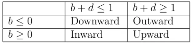
Table 1 shows that nature of the sender’s bias for different values of the parameters
b and d.
b+d≤1 b+d≥1
b≤0 Downward Outward
b≥0 Inward Upward
Table 1: Nature of the sender’s bias for different values of b and d.
Crawford and Sobel (1982) studied in detail the case where b >0 and d= 1 as an
example ofstrictly upward bias and gave an explicit solution. We give here an explicit
solution for all values of the parameters, using their difference equation method.
In equilibrium, a cutoff typexh must be indifferent between inducing the receiver’s reaction to information the interval [xh−1, xh] and the receiver’s reaction to the
infor-8We constructed a continuous path between the equilibrium of the first game and the equilibrium
of the second game. Along the path, the indirect utility of the receiver decreases. An alternative strategy would be to consider a continuous path v from the preference1 to the preference 2,
indexed byv∈[1,2], and such that for allv < v0, the preferencev0 has a strictly pairwise upward
bias with respect tov.We can then consider the greatest equilibrium of sizeκfor each of the games
(R,v), which defines a pathv7→xv in Z
κ∩Xκ.By Corollary 1, the pathxv is decreasing. If the
pathxvis also continuous, then by Lemma 14, the indirect utility of the receiver is decreasing along