Development Of A High Performance Mosaicing And Super-Resolution Algorithm

(1)

University of North Dakota

UND Scholarly Commons

Theses and Dissertations Theses, Dissertations, and Senior Projects

1-1-2015

Development Of A High Performance Mosaicing

And Super-Resolution Algorithm

Debabrata Ghosh

Follow this and additional works at:https://commons.und.edu/theses

Part of theElectrical and Computer Engineering Commons

This Dissertation is brought to you for free and open access by the Theses, Dissertations, and Senior Projects at UND Scholarly Commons. It has been accepted for inclusion in Theses and Dissertations by an authorized administrator of UND Scholarly Commons. For more information, please contact [email protected].

Recommended Citation

Ghosh, Debabrata, "Development Of A High Performance Mosaicing And Super-Resolution Algorithm" (2015).Theses and Dissertations. 1896.

(2)

DEVELOPMENT OF A HIGH PERFORMANCE MOSAICING AND SUPER-RESOLUTION ALGORITHM

by

Debabrata Ghosh

A Dissertation

Submitted to the Graduate Faculty

of the

University of North Dakota

in partial fulfillment of the requirements

for the degree of

Doctor of Philosophy

Grand Forks, North Dakota December

(3)

ii

(4)

iii

This dissertation, submitted by Debabrata Ghosh in partial fulfillment of the requirements for the Degree of Doctor of Philosophy from the University of North Dakota, has been read by the Faculty Advisory Committee under whom the work has been done and is hereby approved.

__________________________________________ Naima Kaabouch, PhD __________________________________________ Saleh Faruque, PhD __________________________________________ William Semke, PhD __________________________________________ Wen-Chen Hu, PhD __________________________________________ Ronald Fevig, PhD

This dissertation is being submitted by the appointed advisory committee as having met all of the requirements of the School of Graduate Studies at the University of North Dakota, and is hereby approved.

_______________________________________________ Wayne Swisher,

Dean of the Graduate School

_______________________________________________ Date

(5)

iv PERMISSION

Title Development Of A High Performance Mosaicing And Super-resolution

Algorithm

Department Electrical Engineering

Degree Doctor of Philosophy

In presenting this dissertation in partial fulfillment of the requirements for a graduate degree from the University of North Dakota, I agree that the library of this University shall make it freely available for inspection. I further agree that permission for extensive copying for scholarly purposes may be granted by the professor who supervised my dissertation work or, in his absence, by the chairperson of the department or the dean of the Graduate School. It is understood that any copying or publication or other use of this dissertation or part thereof for financial gain shall not be allowed without my written permission. It is also understood that due recognition shall be given to me and to the University of North Dakota in any scholarly use which may be made of any material in my dissertation.

Debabrata Ghosh 07/03/2015

(6)

v

LIST OF FIGURES

Figure Page

1.1 Applications of super-resolution mosaicing ... 1

2.1 Different steps of image mosaicing ... 6

2.2 Classification of mosaicing based on registration ... 9

2.3 Candidate feature detection for FAST algorithm... 15

2.4 Scale space formation and extrema finding ... 18

2.5 Approximation of Gaussian second order partial derivatives ... 20

2.6 Use of cross-power spectrum to detect transformation... 23

2.7 Classification of mosaicing based on blending ... 25

2.8 Image blending results ... 27

2.9 Pyramid formation for blending... 28

3.1 A framework of multi-frame super-resolution ... 33

3.2 Observation model relating LR image with HR image ... 35

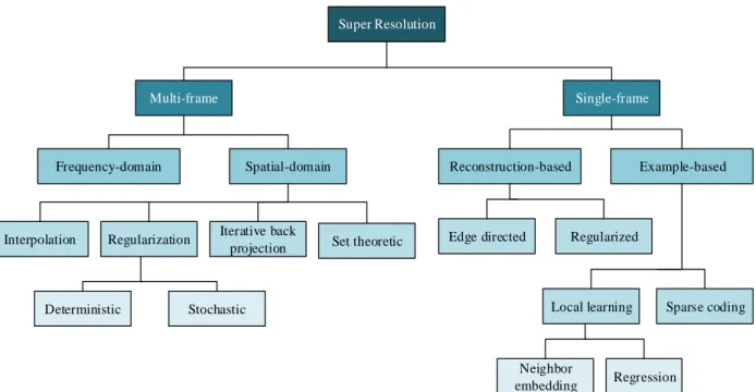
3.3 Taxonomy of super-resolution algorithms ... 37

3.4 Interpolation-based super-resolution reconstruction ... 40

3.5 Iterative back projection ... 48

4.1 Flowchart of the mosaicing algorithm ... 59

4.2 Schematic of the mosaicing algorithm’s evaluation process ... 63

4.3 Matching performance vs distance threshold at different values of BBF NN bins for an example image pair ... 65

(10)

ix

4.4 Matching performance vs number of BBF NN bins at different distance

threshold values for an example image pair ... 66

4.5 Performance vs computation of the RANSAC algorithm at a constant distance threshold value for an example image pair ... 67

4.6 Distance threshold vs computation of the RANSAC algorithm at a constant probability of model corruption for an example image pair ... 68

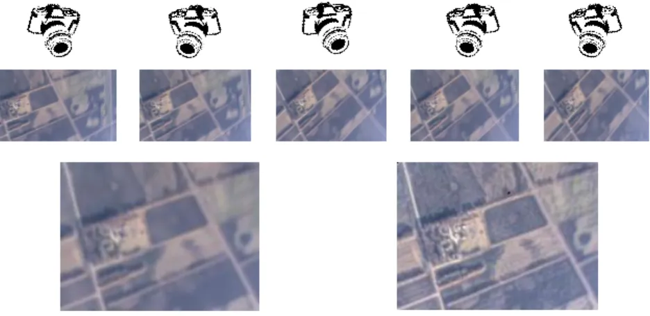
4.7 Input frames for the mosaicing algorithm ... 68

4.8 SIFT features extracted from the input frames ... 69

4.9 SIFT features matching from pair of input frames ... 69

4.10 Projection of frames into common coordinate ... 70

4.11 Step-by-step stitching process... 71

4.12 Mosaicing using an example 2D scene dataset ... 72

4.13 Mosaicing using an example 3D scene dataset ... 73

4.14 Mosaicing using an example UAV dataset ... 73

5.1 Flowchart of super-resolution algorithm ... 84

5.2 Regularization parameter vs number of iterations ... 91

5.3 SR result using simulated balloon data ... 92

5.4 Detailed regions cropped from SR results using simulated balloon data ... 93

5.5 SR result using simulated UAV data ... 95

5.6 Detailed regions cropped from SR results using simulated UAV data ... 96

5.7 SR result using real UAV data ... 97

(11)

x

5.9 Behavior of performance metrics in the presence of blur ... 100

5.10 Behavior of performance metrics in the presence of noise ... 101

5.11 Output CPBD values for five real datasets using different

super-resolution mosaicing algorithms ... 102

5.12 Reciprocal singular value curves for a single dataset

(12)

xi

LIST OF TABLES

Table Page

2.1 Comparative overview of different categories of mosaicing methods

based on image registration ... 24

2.1 Comparative overview of different categories of mosaicing methods based on image blending ... 30

3.1 Comparative overview of different multi-frame super-resolution algorithms ... 49

3.2 Comparative overview of different single-frame super-resolution algorithms ... 58

4.1 Mosaicing algorithm assessment ... 75

5.1 MSE, PSNR, SVD, and SSIM values of different super-resolution mosaicing results using high-altitude balloon frames ... 94

5.2 MSE, PSNR, SVD, and SSIM values of different super-resolution mosaicing results using blurry UAV frames ... 96

5.3 CPBD and RSV values of different super-resolution mosaicing results using real UAV frames ... 99

(13)

xii

ACKNOWLEDGEMENTS

First and foremost I want to thank my advisor Dr. Naima Kaabouch. I appreciate all her

contributions of time, ideas, and funding to make my Ph.D. experience productive and stimulating.

I am also thankful to the other members of my advisory committee:Dr. Saleh Faruque, Dr. William

Semke, Dr. Wen-Chen Hu, and Dr. Ronald Fevig for their helpful feedback and support during

this process.

Lastly, I would like to thank my parents and brother for all their love and encouragement.

I am grateful to my loving, supportive, encouraging, and patient wife Soumita Ghosh whose

(14)

xiii ABSTRACT

In this dissertation, a high-performance mosaicing and super-resolution algorithm is described.

The scale invariant feature transform (SIFT)-based mosaicing algorithm builds an initial mosaic

which is iteratively updated by the robust super resolution algorithm to achieve the final

high-resolution mosaic. Two different types of datasets are used for testing: high altitude balloon data

and unmanned aerial vehicle data. To evaluate our algorithm, five performance metrics are

employed: mean square error, peak signal to noise ratio, singular value decomposition, slope of

reciprocal singular value curve, and cumulative probability of blur detection. Extensive testing

shows that the proposed algorithm is effective in improving the captured aerial data and the

(15)

1

CHAPTER 1 INTRODUCTION

There are various applications of super-resolution mosaicing, including surveillance,

disaster management, and urban mapping. Example results of super-resolution mosaicing relevant

to the aforementioned applications are shown in Figure 1.1. The two-fold benefit of

super-resolution mosaicing is obvious: 1) instead of processing each and individual frames to analyze a

certain scene, this technique gives the advantage of processing a single integral frame, thus it saves

significant processing time and 2) higher spatial resolution output of this technique provides the

advantage of better content visualization, which is critical in all of the aforementioned applications.

Figure. 1.1: Applications of super-resolution mosaicing. (a) Application in surveillance; (b) Application in disaster management; (c) Application in urban mapping.

(a) (b)

(16)

2

Higher the quality of the images, better the spatial resolution. The sensor size and detector

density primarily determine the spatial resolution of the captured images. Larger the size of the

sensor, and/or the higher the density of the detectors, the better the spatial resolution of the acquired

images. The most direct hardware-based approach of increasing the spatial resolution is to reduce

the detector size or, equivalently, to increase the detector density. Alternatively, the sensor size

can also be increased. However, smaller detectors have lower dynamic range, lower fill factor,

lower light sensitivity, higher dark signal, higher diffraction sensitivity, and higher non-uniformity

[1]. In addition, the hardware cost increases with both the increase of detector density and sensor

size. Thus, the aforementioned hardware-based approach often restricts the maximum achievable

resolution of the captured images. Besides the sensor-imposed restriction, there are several other

factors that limit the quality of the captured images, including lens and atmospheric blurs, finite

shutter speed, finite aperture, movement of objects in the scene, sensor noise, and media turbulence

[2]. Similarly, the frames lose spatial resolution during video acquisition due to sensor array

sampling. Some of these limitations can be overcome by employing computationally intensive

image processing algorithms that require high processing time and high-power computers, making

them unsuitable for low to medium budget systems.

In order to overcome the limitations inherent in the commercially available affordable

electronics, an approach that combines the available optics and a resolution-enhancement

algorithm can be used. This technique would overcome the final specification restrictions of the

commercial optics. The aim of this dissertation is to develop an efficient, robust and automated

(17)

3

computational resources. Other than increasing the field of view of commercial imagers, the

mosaicing algorithm will add further benefit of eliminating redundant data from overlapping

frames, which are required as input for the high-resolution algorithm. The essential steps required

for the proposed super-resolution mosaicing are image mosaicing and super-resolution.

Super-resolution reconstruction algorithm (SR) creates a high-resolution (HR) image from

a sequence of correlated low-resolution images of the same scene taken from different viewpoints.

Since super-resolution increases the spatial resolution by taking advantage of more samples than

those found in any single low-resolution image, the presence of motion among the low-resolution

images is compulsory for the success of this method. The reconstruction primarily relies on the

ability to estimate the aforementioned motion between frames to recover details that are finer than

the sampling grid. Simultaneously the effects of blur, noise, and other artifacts are eliminated in

the reconstruction process.

Image mosaicing, on the other hand, is the alignment of multiple correlated images into a

wider composition. Mosaicing is a special case of scene building where the images are related by

planar homography only. This is a reasonable assumption if the images exhibit no parallax effects,

i.e. when the scene is approximately planar or the camera purely rotates about its optical center.

Using mosaicing, it is possible to extend the field of view of a camera by preserving the original

resolution and without introducing undesirable lens deformation.

Combining image mosaicing and super resolution becomes a powerful means to represent

all the information on multiple overlapping images and obtain a high-resolution panoramic view

(18)

4

simultaneously generate mosaic output with an improved spatial resolution. This method is

referred to as super-resolution mosaicing. The stability of a super-resolution mosaicing method

necessitates that the overlapping images are correlated solely by planar homography, which is

fulfilled readily in small satellite applications since the captured images from high altitude do not

suffer from parallax effects.

In this dissertation, we will describe a super-resolution mosaicing algorithm and compare

its performance with those of other well-known state-of-the-art algorithms. The dissertation is

organized as follows: Chapter 2 presents an introduction to image mosaicing framework and

reviews the state-of-the-art of image mosaicing techniques. A classification of the techniques is

also proposed, highlighting the benefits and drawbacks of different methods. Chapter 3 presents

an introduction to super-resolution framework along with the image observation model that has

been used in most resolution algorithms. A detailed survey of the state-of-the-art

super-resolution techniques by classifying them into several categories is also presented. Chapter 4

details the proposed mosaicing technique. All the steps involved, including registration,

reprojection, and stitching are described. Finally, some experimental results, based on large

datasets, are presented. Chapter 5 presents the proposed super-resolution mosaicing approach in

detail. Some experimental results are also discussed and compared to results obtained by other

state-of-the-art approaches. Chapter 6 presents the conclusions of this work, and identifies some

(19)

5

CHAPTER 2 STATE-OF-THE-ART OF IMAGE MOSAICING METHODS

2.1 Introduction

Image mosaicing is the alignment of multiple overlapping images into a large composition

which represents a part of a 3D scene [3]. Mosaicing could be regarded as a special case of scene

reconstruction where the images are related by planar homography only [4]. This is a reasonable

assumption if the images exhibit no parallax effects, i.e. when the scene is approximately planar

or the camera purely rotates about its optical center [5]. Using mosaicing it is possible to extend

the field of view (FOV) of a camera by preserving the original resolution and without introducing

undesirable lens deformation [6]. There have been a variety of new additions to the classic

applications of image mosaicing that primarily aim to augment the FOV. Mosaic construction is

finding its practices in many computer vision and computer graphics applications, such as motion

detection and tracking [7-9], mosaic-based localization [10,11], resolution enhancement [12-14],

augmented reality [15, 16] etc. Furthermore, video compression [17], video indexing [18], and

image stabilization [19] are some of the prominent areas where mosaicing is creating significant

impacts.

As shown in Figure 2.1, mosaicing involves various steps of image processing: registration,

reprojection, stitching, and blending. Registration refers to the establishment of geometric

correspondence between a pair of images depicting the same scene. In order to register a set of

(20)

6

respect to a reference image within that set. The set may consist of two or more images taken of a

single scene at different times, from different viewpoints, and/or by different sensors. The most

general case of the transformation is the 8 degree of freedom planar homography [3]. The next

step, following the registration, is reprojection which refers to the alignment of the images into a

common coordinate system using the computed geometric transformations. The goal of the

stitching step is to overlay the aligned images on a larger canvas by merging pixel values of the

overlapping portions and retaining pixels where no overlap occurs. Errors propagated via

geometric and photometric misalignments often result in undesirable object discontinuities and Figure. 2.1: Different steps of image mosaicing. Here H are the homography matrices between source images.

(21)

7

seam visibility in the vicinity of the boundary between two images. Thus, a blending algorithm

needs to be used during or after the stitching step in order to minimize the discontinuities in the

global appearance of the mosaic.

Image mosaicing is an attractive research area, which has resulted in the development of

many algorithms in the literature [12,20-34]. A comprehensive review of the existing algorithms

will undoubtedly be a valuable guide to researchers and developers for selecting a suitable image

mosaicing method for a specific application. The continuous emergence of new algorithms in

recent years further reinforce the necessity of such a comprehensive review. In the following

sections, we classify the past and current mosaicing techniques based on image registration as well

as image blending. For each of these classifications, we provide a comprehensive review of the

major categories of the image mosaicing methods. In addition, this review highlights the evolving

paths of those methods by providing the modifications that have been made to those basic methods

by different researchers.

Both registration and blending directly influence the performance of image mosaicing.

Being the first and last step of image mosaicing, it is almost impossible to build a successful

mosaicing algorithm without correctly implementing registration and blending algorithms. Though

attempts have been made to overcome the registration errors by utilizing sophisticated blending

algorithms, the significance of accurate registration in image mosaicing remains unquestionable.

In this chapter, we focus on the classification of the existing image mosaicing algorithms based on

their registration methods, as well as based on their blending methods.

(22)

8

Image registration is not only an important step of image mosaicing, but also is the

foundation of it. Registration of multi-source images, which are focused on the same target but

produced from different sensors, different perspective, and different times, computes the optimal

geometric transformation by looking into the correspondences between each pair of images. This

process makes the multi-source images aligned into a common reference frame using the estimated

geometric transformations. To the extent that corresponding points from multi-source images are

aligned together, the registration is successful [41]. The aforementioned correspondences can be

established by matching templates between images, or by matching features extracted either from

images, or by utilizing the phase correlation property in the frequency domain.

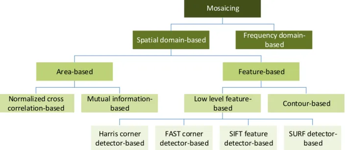
As shown in Figure 2.2, based on image registration methods, image mosaicing algorithms

can be spatial domain-based or frequency domain-based. Spatial domain-based image mosaicing

can further be grouped into area-based image mosaicing and feature-based image mosaicing.

Feature-based image mosaicing can again be subdivided into low-level feature-based image

mosaicing and contour-based image mosaicing. Low-level feature-based mosaicing can be divided

into four classes: Harris corner detector-based mosaicing, FAST corner detector-based mosaicing,

SIFT feature detector-based mosaicing, and SURF detector-based mosaicing. Different classes of

(23)

9 Mosaicing Frequency domain-based Spatial domain-based Area-based Feature-based Normalized cross correlation-based Mutual information-based

Low level

feature-based Contour-based Harris corner detector-based FAST corner detector-based SIFT feature detector-based SURF detector-based

2.2.1 Spatial domain image mosaicing methods

Algorithms in this category use properties of pixels to perform registration, and, thus they

are the most direct methods of image mosaicing. Majority of the existing image mosaicing

algorithms fall into this category. Spatial domain-based image mosaicing can be either area-based

or feature-based. Area-based image mosaicing algorithms rely on computation between “windows” of pixel values in the two images, which need to be mosaicked [42]. The fundamental

approach is to shift the “windows” of the images relative to each other and see how much the

pixels match. Subsequently, transformation parameters are obtained and used to warp and stitch

the images. Unlike area-based image mosaicing, feature-based mosaicing methods use

feature-to-feature matching in order to compute the geometric transformation between a pair of images. Thus,

these methods rely primarily on feature extraction algorithms which can detect salient features Figure 2.2: Classification of mosaicing based on registration.

(24)

10

from the images. Salient features are subsets of the image domain, often in the form of isolated

points, continuous curves or connected regions [49]. Since the features are used as the starting

point, the overall algorithm will often be as good as the feature extraction algorithm is.

Two of the most commonly used area-based image mosaicing algorithms are normalized

cross correlation-based mosaicing and mutual information-based mosaicing. Based on the types of

features extracted, based mosaicing methods can also be classified into low-level

feature-based mosaicing and contour-feature-based mosaicing. Again, feature-based on popular low-level feature

extraction methods, low-level feature-based mosaicing can be subdivided into the following

categories: Harris corner detector-, Features from Accelerated Segment Test (FAST)-, Scale

Invariant Feature Transform (SIFT)-, Speeded Up Robust Feature (SURF)-based mosaicing

methods. These above-mentioned classes of mosaicing algorithms are described below.

2.2.1.1 Normalized Cross Correlation (NCC)-based mosaicing

This method computes similarity between the “windows” in the two images for each shifts.

It is defined as [43]: ( ) ( ) ( ) 2 2 ( ) ( ) U x U V x u V i _i _i NCC u U x U V x u V i _i _i  _   _{ }         _   _{ }       (2.1) where U 1 U x( ) i N i   (2.2) V 1 V x( u) i N i    (2.3)

(25)

11

where U _andV _{are the mean images of the corresponding “windows”,}U _andV _{for the first}

and second images respectively. N is the number of pixels in the “window”,xi ( , )x yi i is the pixel coordinate in the “windows”, u( , )u v _{is the displacement or shift where NCC coefficient is}

calculated. The NCC coefficient values are always within the range [-1, 1]. The shift parameter

corresponding to the peak NCC value represents the geometric transformation between the two

images. Once geometric transformations are obtained between the image pairs, images are warped

in the reference frame, and finally stitching is performed to generate the final mosaic. Methods

within this category have the advantage of being computationally simple, however, at the cost of

being particularly slow. Moreover, they perform accurately only when there are significant

overlapping between the source images.

Several techniques [22,44-46] have been proposed to tackle the above mentioned problems.

In order to make the computation faster, Berberidis et al. [44] proposed an iterative algorithm for

the spatial cross correlation in order to compute the displacements between the source images. Yet

another method based on adjusting the correlation windows according to the scale and orientation

of extracted interest-points from the source images was proposed by Zhao et al. [45] to increase

the computation speed. In order to improve the performance of the algorithm in the presence of

non-rigid deformation, Vercauteren et al [46] suggested the use of Riemannian statistics along with

a scattered data fitting-based mosaicing. Nasibov et al. [22] employed a brightness correction

matrix before the registration step in order to make the algorithm less sensitive to the illumination

(26)

12

2.2.1.2 Mutual Information (MI)-based mosaicing

Unlike NCC, which computes similarity based on image intensity values, mutual

information measures similarity based on the quantity of information shared between two images.

MI between two images I1_andI2_{is expressed in terms of entropy as:}

1 2 1 2 1 2

( , ) ( ) ( ) ( , )

MI I I E I E I E I I _(2.4)

where E I( )1 _andE I( 2)_{are the entropies of}I1_andI2_{, respectively. And}E I I( ,1 2)_{represents the joint}

entropy between the two images. Entropy is a measure of variability of a random variable. Thus

variability of I1_{is expressed as:}

1 1 1 ( ) _I( ) log( _I ( )) g E I  



p g p g (2.5)

wheregare the possible gray level values of I1_{, and accordingly} pI1( )g is the probability

distribution function ofg. Similarly, the joint variability of I1_andI2_{is expressed as:}

1 2 1 2 1 2 _, , , ( , ) _{I I} ( , ) log( _{I I} ( , )) g h E I I  



p g h p g h (2.6)

whereh_{indicates the possible gray level values of}I2_.pI I1,2( , )g h is the joint probability distribution

function of gand h_{. Typically, the joint probability distribution between two images is measured}

as normalized joint histogram of the gray level values. It is observed that better the alignment

between two images, higher the MI between them. Thus, two images are geometrically aligned by

a transformation if the MI between them is maximum for that transformation. After the appropriate

transformations are obtained between the image pairs, they are reprojected and stitched to get the

(27)

13

occlusion changes between source images. However, similar to NCC-based methods, these

techniques have the disadvantages of being computationally slow, and requiring high degree of

overlapping between input images.

A number of techniques [24,47,48] have been proposed to address its shortcomings. To

increase the computation speed, Dame et al. [47] employed a B-spline function for normalized

mutual probability density, in combination with Newton’s method for optimizing the MI cost

function. Another method presented by Luna et al. [24]uses a stochastic gradient optimization

along with MI-based similarity measure in order to make the algorithm faster. Concerning the

drawback of MI-based mosaicing algorithms for low overlapping images, Césare et al. [48]

proposed a template matching approach capable of explicitly acknowledging the plausibility of

similarity between distant neighborhoods, and delaying definite block-to-block association to a

step that globally evaluates their collective likelihood.

2.2.1.3 Harris corner detector-based mosaicing

Harris corner detector detects corner points as robust low-level features from source

images. Initially a local detection window in an image is chosen. Subsequently the variation in

intensity that results by shifting the window by a small amount in different direction is determined

as below [39]: 2 , ( , ) ( , ) [ ( , ) ( , )] x y E u v 



w x y  I x u y  v I x y (2.7)

(28)

14

where w x y( , )is the window function, I x y( , )is the image intensity value at pixel location( , )x y ,

( , )

I x u y v  _{is the shifted intensity with}( , )u v _shift,_{is the convolution operator. The local texture}

around pixel ( , )x y is expressed as autocorrelation matrix C_{as below:}

2 2 , ( , ) x x y x y x y y I I I C w x y I I I          



(2.8)

where Ix_and Iy_{are the first derivative of} I x y( , )_{. Two large eigenvalues for the matrix} C

corresponds to a corner point. The center point of the window is characterized as a corner point. For more robustness, a “cornerness” measure R_{is used to eliminate the edge points as below [25]:}

2

( ) ( )

RDet C Tr C (2.9)

where Tr C( )is the trace of C_and _{is within the range}0.04  0.06_{. Corner points are detected}

as local maxima of R_{above a predefined threshold}T_{. After the Harris corner points are detected}

from both the images, correspondences are established either by NCC or by any other Sum of

Squared Difference (SDD) method. Subsequently, the geometric motion parameters are calculated

and images are warped into a global reference frame in order to stitch them all. Mosaicing

algorithms using Harris corner detector are computationally simple and accurate.

One major problem with the Harris corner detector-based mosaicing methods is that large

changes in rotation often generates ghosting in the mosaic output. [25] dealt with this by utilizing

a luminance center-weighting algorithm which is used following a slope clustering algorithm for

Harris corner point matching. Another problem related to the uncertainty in choosing a local

(29)

15

matching in order to limit the search window to potential homologous points. Harris corner

detector almost always finds closely crowded feature points. However, this can be overcome by

counting the number of feature points in the neighborhood and then accordingly exclude some of

the points, as has been done in [26].

2.2.1.4 FAST corner detector-based mosaicing

FAST algorithm is a corner detection algorithm which is computationally more efficient

and faster than most of the other low-level feature extraction methods; thus mosaicing methods

based on this algorithms are particularly suitable for real-time image processing applications.

Initially a circle of sixteen pixels is considered around each corner candidate. According to the

FAST algorithm, the candidate is a corner if there exists a set of n_{contiguous pixels in the circle}

which are all brighter than the intensity of the candidate pixel plus a threshold, or all darker than

the intensity of the candidate pixel minus the threshold, as shown in Figure 2.3. The numbern_is

usually chosen twelve. In order to increase the computational speed of FAST algorithm, a corner

response function (CRF) is used. CRF gives the numerical value of the “cornerness” of a corner Figure 2.3: Candidate feature detection for FAST algorithm.

(30)

16

point based on image intensities in the local neighborhood [39]. Corners are detected as local

maxima for the CRF function computed over the entire image. Following the detection, corner

point matching is performed for each pair of frames. Sometimes a Bag-of-Words (BoW) algorithm

is used to represent each image as a set of corner descriptors to speed up the matching process as

in [27]. Then, homography matrices are computed and finally the images are projected into a

common coordinate to get the final mosaic.

Choosing an optimal threshold is often a fundamental challenge of the FAST corner

detector-based algorithms. However, it can be addressed by incorporating a robust threshold

selection algorithm as in [53]. For matching the corner points from successive frames, they further

proposed a threshold learning method together with a region-based gray correlation. Another major

issue of the FAST-based algorithms is that they are not particularly robust to increased degree of

variations. For that, extending the sampling area beyond the sixteen pixels around each candidate

point [52] could be considered as a promising approach, since it gives the FAST corner points

more distinctiveness and, in turn, makes them invariant to larger variations.

2.2.1.5 SIFT feature detector-based mosaicing

SIFT algorithm is a low-level feature detection algorithm which detects distinctive features (also called “keypoints”) from images. The SIFT descriptor is invariant to translations, rotations

and scaling transformations in the image domain and robust to moderate perspective transformations and illumination variations. SIFT’s operation is based on five major steps:

scale-space construction, scale-scale-space extrema detection, keypoint localization, orientation assignment,

(31)

17

repeatedly using a Gaussian filter with changing scales and grouping the outputs into octaves as

[54]:

( , , ) ( , , )* ( , )

L x y G x y I x y (2.10)

where * is the convolution operator, G x y( , , ) is a Gaussian filter with variable scale  , and I x y( , )

is the input image. After the scale space construction is complete, difference-of-Gaussian (DoG)

images are computed from adjacent Gaussian-blurred images in each octave as [54]:

( , , ) ( , , ) ( , , )

D x y L x y k L x y (2.11)

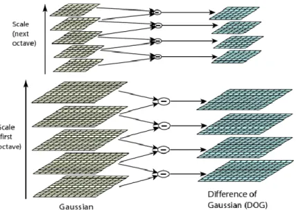
Following that, candidate keypoints are identified as local extrema of DoG images across

the scales. The scale space and DoG scale space construction as well as extrema detection in DoG

scale space is illustrated in Figure 2.4. In the next step, low contrast keypoints and edge response

points along the edges are discarded using accurate keypoint localization. The keypoints are then

assigned one or more orientations based on local image gradient directions as [54]:

1

( , )x y tan (( ( ,L x y 1) L x y( , 1)) / ( (L x 1, )y L x( 1, )))y

 _  _{ } _ _ _ _ _(2.12)

where ( , )x y represents the gradient direction for L x y( , , ) . A set of orientation histograms is

formed over the neighborhoods of each keypoint. Finally, a normalized 128-dimensional vector is

(32)

18

from two images, nearest neighbor of a keypoint in the first image is identified from a database of

keypoints for the second image [54, 55]. Following the initial matching, RANSAC algorithm is

used to remove the outliers and to compute the transformation parameters between a pair of frames.

Finally, images are warped using the transformation parameters and stitched to generate the mosaic

image. SIFT based image mosaicing algorithms are particularly suitable for stitching high

resolution images under variety of changes (rotation, scale, affine etc.), however, at the cost of

high processing time.

Several researchers have made variations to the above mentioned SIFT-based mosaicing

method in order to further improve its performance. For example, in [12] the authors proposed

switching between Kanade-Lucas-Tomasi (KLT) tracker and SIFT matching to find the

correspondences between successive frames depending on their amount of overlapping. In [28], Figure 2.4: Scale space formation and extrema finding. (a) Scale space and DoG scale space construction; (b)

(33)

19

the author exploited a deformation vector propagation algorithm in the gradient domain to reduce

the intensity discrepancy between the mosaiced images. Similarly, a bundle adjustment algorithm

along with a modified-RANSAC algorithm capable of developing a probabilistic model is used in

[56] to eliminate registration error and make the matching process more accurate.

2.2.1.6 SURF feature detector-based mosaicing

SURF algorithm is a scale and rotation invariant local feature detector. Like SIFT, this

algorithm is also based on scale space theory. However, SURF uses Hessian matrix of the integral

image to estimate local maxima across different scale spaces [57]. The Hessian matrix of an image

I with scale  at any point X( , )x y is defined as [58]:

( , ) ( , ) ( , ) ( , ) ( , ) xx xy xy yy L X L X H X L X L X         _ _   (2.13)

where Lxx( , )X  _,Lyy(X, ) _{, and}Lxy(X, ) _{are the convolutions of}I _{in point}X_{with Gaussian second}

order filters 2 2G( ) x    _, 2 2G( ) y    , and 2 ( ) G x y  

  _{respectively. While computing Hessian matrix at}

each pixel, the Gaussian filter operations are approximated by operations using box filters as

shown in Figure 2.5. The response at each pixel is computed as the determinant of the Hessian

matrix. Following that, a thresholding and a 3 x 3 x 3 local maxima detection window are used for

non-maxima suppression. The local maxima are then interpolated in scale space to achieve

keypoints with their location and scale values. In order to assign orientation for each keypoint,

(34)

20

vector is formed by summing up all the responses within 60-degree window. The longest vector is

assigned as orientation to the keypoint. In order to assign descriptor vector to each keypoint, a

square neighborhood region around the keypoint is selected. It is then split into smaller

sub-regions. Sum of the Haar-wavelet responses from all the sub-regions are then used to generate a

64 dimensional descriptor vector [50]. After finding the matching keypoints from a pair of images,

RANSAC algorithm is used to eliminate false matches as well as to calculate the homography

matrices. Once homography matrices are achieved, images are warped and stitched to get the final

mosaic. SURF based mosaicing techniques are faster than SIFT based techniques. However, they

perform poorly under certain variations (particularly color, illumination, some affine

transformation).

The process of determining the SURF descriptors as mentioned above has sometimes been

modified by some authors. For example, in [59] the local maxima is searched beyond a 3 x 3 x 3

neighborhood in the present scale and two immediately adjacent scales in order to make the feature

descriptors more distinctive. In [60], the authors proposed dividing the SURF descriptor window

into eight sub-regions while assigning descriptor vector. This technique increases the matching Figure 2.5: Approximation of Gaussian second order partial derivatives. (a) Approximation in x direction; (b)

Approximation in y direction; (c) Approximation in xy direction.

(35)

21

speed at the cost of increased false matches. However, the authors show that the use of RANSAC

guarantees elimination of most of those incorrect matches.

Often multiple low-level feature extraction methods are used together in image mosaicing

algorithms in order to use their respective benefits. Joshi et al. [61] propose a mosaicing algorithm

which uses both Harris corner detector and SURF detector for extracting distinctive features from

source images. Feature-based mosaicing algorithm proposed by Bind et al. [62] use both SIFT and

SURF based feature detector to detect interest points from images. Kang et al. [63] and Zhu et al.

[64] use Harris corner detector and SIFT detector in their feature-based mosaicing algorithm.

2.2.1.7 Contour-based mosaicing

This type of mosaicing algorithms is based on extraction of high-level features from

images. Unlike the low-level features, these features are more natural to human perception and

therefore they are high-level. High-level feature extraction mostly concerns finding the shapes or

textures in an image. Shape extraction implies finding their position, orientation and their size [49].

Usually regions of different structures are extracted as high level image features. Then these

features are matched to find correspondences, which are later used to compute the transformation

parameters. Different techniques can be used to eliminate the false matches. Finally, warping and

blending are performed to generate the mosaic output. The use of high-level features significantly

increase the computation in these types of mosaicing algorithms. However, they are particularly

suitable to work under larger and complicated motion parameters, and even under multi-layer

(36)

22

Some of the notable contributions in high-level feature-based mosaicing include [65-67].

In [65], the authors used a wide baseline algorithm together with an adaptive region expansion

method to achieve robust registration using high-level features. Prescott et al. [66] proposed

extracting regions of image structures using a threshold technique and then computing area-based

similarity matching for registration. Contour extraction using a segmentation algorithm, followed

by finding their centroids for image registration was used in [67].

2.2.2 Frequency domain image mosaicing methods

Unlike spatial domain-based image mosaicing algorithms, methods classified in this

category require computation in the frequency domain in order to find the optimal transformation

parameters between a pair of images. These algorithms use the property of phase correlation for

registering images. Let I x y1( , )_andI2( , )x y are two images having some overlapping areas. Let’s

further assume that (x0_,y0_{) is the translation between the images. Thus,}

2( , ) 1( 0, 0)

I x y I xx yy (2.14)

The corresponding Fourier transforms F u v1( , )_andF u v2( , )_{are related by:}

0 0

( )

2( , ) 1( , ).

j ux vy

F u v F u v e  (2.15)

The cross-power spectrum of the two images is defined as: [Ref 54]

0 0 * ( ) 1 2 * 1 2 ( , ) ( , ) ( , ) ( , ) j ux vy F u v F u v e F u v F u v    (2.16)

where F1*( , )u v _{is the complex conjugate of}F u v1( , )_{. The shift theorem guarantees that the phase of}

(37)

23

be solved in two different ways. One way is to work directly in frequency domain. However, this

technique is very sensitive to noise. A better approach is to take inverse Fourier transform of the

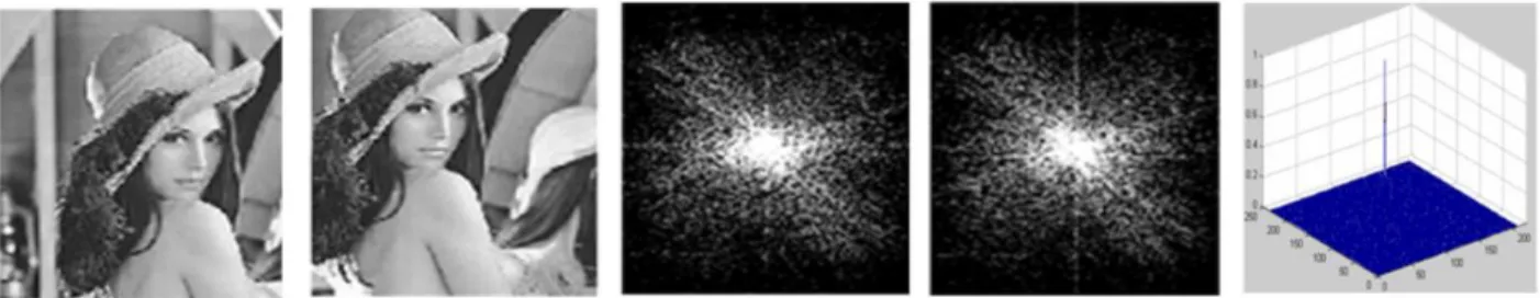
above equation and get an impulse function  (x x y0, y0)_{, which is approximately zero}

everywhere except at the displacement (x y0, 0)_{as shown in Figure 2.6. With the displacement}

(translational) parameters the two images are warped and finally stitched to get a mosaic.

Mosaicing algorithms based on this technique are usually efficient because of the use of shift

property of Fourier transform and the use of Fast Fourier Transform (FFT). However, they suffer

from being overly sensitive to noise. Additionally, accurate registration often requires significant

overlapping between source images.

The above explained method of image mosaicing has sometimes, as in [30,68,69], been

modified to make it suitable for handling transformations other than translation. A two-step

method is proposed in [68]. The first step computes the rotation angle by finding the maximum

peak by rotating the target image with an incremental angle. Using the computed rotation angle

and phase correlation, the second step determines the translational displacement. A log-polar

transformation is utilized in [30] to find the scale and translational parameters. In [69], the authors Figure 2.6: Use of cross-power spectrum to detect transformation. (a), (b) Source images with displacement between them; (c), (d) Corresponding spectrum; (e) Impulse function indicating displacement between the images.

(38)

24

suggested changing the rotation and scale parameters to translational parameters using

Fourier-Mellin transform.

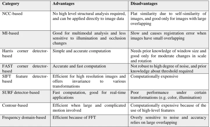
The comparative overview of different categories of mosaicing algorithms based on image

registration is presented in Table 2.1.

Table 2.1: Comparative overview of different categories of mosaicing methods based on image registration

Category Advantages Disadvantages

NCC-based No high level structural analysis required, and can be applied directly to image data

Flat similarity due to self-similarity of images, and good only for images with large overlapping

MI-based Good for multimodal analysis and less sensitive to illumination and occlusion changes

Slow and causes registration error when images have small overlapping

Harris corner detector-based

Simple and accurate computation Needs prior knowledge of window size and good only for moderate changes in scale and rotation

FAST corner detector-based

Accurate and fast computation Not robust to high degree of noise, and prior knowledge about threshold required SIFT feature

detector-based

Efficient for high resolution images and offers invariance to various transformations

Computationally expensive

SURF detector-based Fast computation, good for real-time applications

Poor performance under certain transformations (e.g. color, illumination) Contour-based Efficient when large and complicated

motion involved

Computationally expensive because of the use of high-level features

Frequency domain-based Efficient because of FFT Overly sensitive to noise and accuracy relies on large overlapping

2.3 Classification of image mosaicing methods based on blending

Similar to registration, image blending is also a significant step for successful

implementation of mosaicing. Stitching multiple images together to create a seamless mosaic

(39)

25

registration, which is vital to equalize color and luminance appearance in a composite image. There

are several reasons (differences in camera exposure, scene illumination, or presence of moving

objects between frames or geometric misalignments) which may lead to image inconsistencies in

the final mosaic. The visibility of such inconsistencies can be minimized by choosing appropriate

blending algorithm. This way, the final mosaic would be visibly free of annoying seams, giving it

a more consistent global appearance. Figure 2.7 shows that based on the image blending,

mosaicing algorithms can be transition smoothening-based and optimal seam-based. Transition

smoothening-based mosaicing can be further grouped into feathering-based, pyramid-based, and

gradient-based mosaicing. Different classes of image mosaicing algorithms based on the image

blending methods are discussed below.

Mosaicing

Optimal seam-based Transition

smoothening-based

Feathering-based Pyramid-based Gradient-based

2.3.1 Mosaicing methods using transition smoothing-based blending

Mosaicing algorithms within this category attempt to minimize the visibility of seams by

smoothing the common overlapping regions of the combined images. The information of the

overlapping region between two images is fused in such a way that the boundaries of the images

involved become imperceptible. Even though a totally indistinguishable transition may be Figure 2.7: Classification of mosaicing based on blending.

(40)

26

achieved, the content and coherency of the overlapping region is not guaranteed, as the information

is fused without taking into account the content of the scene [70]. Thus, most often, these

mosaicing methods generate mosaic with blurry transitions in the boundary regions. Popular

methods which use transition smoothing for their blending operation include feathering, pyramid

blending, and gradient-based blending. Mosaicing algorithms based on these techniques are

discussed briefly as follows:

2.3.1.1 Mosaicing algorithms using feathering-based blending

Mosaicing algorithms within this category perform blending operation by taking an

average value in each pixel of the overlapping region. However, the simple average method fails

when exposure differences, misalignments, and presence of moving object are very obvious in the

input images. A better approach to the averaging method is to use weighted averaging along with

a distance map. Pixels near the center of an image are weighted heavily and those near the edges

are weighted lightly. This is done by computing a distance map in terms of Euclidean distance of

each valid pixel (mask) from its nearest invalid pixel as [43].

~ ( ) arg min{ ( ) } k k y w x  yy I xy is invalid (2.17) where ~ ( ) k

I x _{are the warped images and}w x_k( )

are the weights of the images. Finally, the mosaic

image is generated as a weighted combination of the input images. Examples of composite images

formed of six color images using simple average blending and feathering are shown in Figure 2.8.

(41)

27

exposure differences. However, it is difficult in practice to achieve a balance between smoothing

out low-frequency exposure differences and preserving sharp enough transitions to prevent

blurring. Furthermore, these methods suffer from ghosting effect.

Examples of mosaicing methods using feathering-based blending include [56] [71] and

[60]. [56] and [71] used alterations of the above mentioned method for finding the weights of

images in the overlapping region. In [56]. the aforementioned weight is measured by computing

the distance of the overlapping pixels from the borders of the left and the right images. In [71], the

authors used weighted average of the pixel color values in the overlapping region.

2.3.1.2 Mosaicing algorithms using pyramid-based blending

In an attempt to perform the blending operation in a more robust way, these mosaicing

algorithms convert the input images into band-pass pyramids as shown in Figure 2.9. Mask image

associated with each source image is then created. Mask creation can be made automatic by using

grassfire transform as used in [72]. Then the mask image is converted into a low-pass pyramid by

using a Gaussian kernel [43]. The resultant blurred and subsampled masks are treated as weights

to perform per-level feathering. The final mosaic is then achieved by interpolating and summing

the results from per-level feathering as:

Figure 2.8: Image blending results. (a) Blending using simple averaging; (b) Blending using feathering. (a) (b)

(42)

28

1 2

( , ) ( , )* ( , ) (1 ( , ))* ( , )

LO x y GM x y LI x y  GM x y LI x y (2.18)

where LI x y1( , )_and LI2( , )x y _{are the Laplacian pyramids of the warped source images}I1_and I2_.

( , )

GM x y _{is the Gaussian pyramid of the mask image}M x y( , )_andLO x y( , )_{is the Laplacian pyramid}

of the output image O x y( , ). Sometimes, all the strips are combined in a single blending step when

it needs building pyramids for multiple narrow strips as proposed in [31]. Algorithms using the

above method achieve reasonable balance between smoothing out low frequency components and

preserving sharp enough transitions to prevent blurring [74]. Edge duplication is also eliminated

noticeably. However, double contouring and ghosting effects become significant when the

registration error is significant.

2.3.1.3 Mosaicing algorithms using gradient-based blending

Another group of transition smoothening method are those based on gradient domain

blending. These methods are based on the idea that by suitably mixing the gradient of images, it is

possible to mosaic image regions convincingly. In general the gradients across seams are set to

zero for smoothing out the color differences. Since humans are more sensitive to gradients than

image intensities, mosaicing methods using this technique generate visually more pleasant results (a) (b)

(43)

29

compared to the other two techniques discussed before. However, working exclusively in the

gradient domain requires higher computational resources to deal with large data sets. Furthermore,

for best performance, the alignment of images through registration needs to be almost perfect.

Notable work in this group was developed by [32], [75], and [76]. In [75], the authors used

a gradient domain object moving and region filling algorithm to eliminate the visible artifacts

arising from moving objects in the scene. Algorithm based on assigning low resolution offset map to each source image followed my Poisson’s blending was proposed by Szeliski et al. [76]. In [32],

the authors developed two approaches called GIST (gradient domain image stitching). One of the

approaches is based on minimizing a cost function that evaluates the dissimilarity measure between

the derivatives of the mosaic and the derivatives of the source images. The other approach is based

on inferring a mosaic by optimization over image gradients.

2.3.2 Mosaicing methods using optimal seam-based blending

This type of mosaicing algorithms attempt to minimize the visibility of seams by looking

for optimal seams in the joining boundaries between the images. The objective of optimal seam

technique is to allocate the optimal location of a seam line by looking into the overlapping region

between a pair of images. The seam line placement should be such that it minimizes the

photometric differences between the two sides of the line. At the same time the seam line should

be able to determine the contribution of each of the images in the final mosaic. Once the placement

and the contribution information are obtained, each image is copied to the corresponding side of

the seam. When the difference between the two images on the seam line is zero, no seam gradients

(44)

30

blending, optimal seam-based mosaicing algorithms consider the information content of the scene

in the overlapping region, allowing to deal with problems like moving objects or parallax.

However, no information is fused in the overlapping region, thus the transition between the images

can be easily noticeable when there are global intensity or exposure difference between the frames.

Different optimal seam finding methods have been used in mosaicing literature. For

example, in [33] a modified region-of-difference method is used.[77] proposed the use of an

algorithm based on watershed segmentation and graph cut optimization. Another method based on

dynamic programming and grey relational analysis is used in [78].

A general comparison of different categories of mosaicing algorithms based on image

blending is presented in Table 2.2.

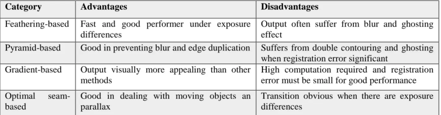
Table 2.2: Comparative overview of different categories of mosaicing methods based on image blending

Category Advantages Disadvantages

Feathering-based Fast and good performer under exposure differences

Output often suffer from blur and ghosting effect

Pyramid-based Good in preventing blur and edge duplication Suffers from double contouring and ghosting when registration error significant

Gradient-based Output visually more appealing than other methods

High computation required and registration error must be small for good performance Optimal

seam-based

Good in dealing with moving objects an parallax

Transition obvious when there are exposure differences

(45)

31

CHAPTER 3 STATE-OF-THE-ART OF IMAGE SUPER-RESOLUTION METHODS

3.1 Introduction

Super-Resolution (SR) is the process of achieving a high-resolution (HR) image from a

single low-resolution (LR) observation or a sequence of LR observations of a scene taken at

different viewpoints. It aims to overcome the limitations of the image capturing devices to produce

a high resolution image. In SR context, HR means higher spatial resolution and hence higher

information content. HR images are not only visually appealing, but also valuable in several

practical applications for extracting additional details. SR has been an active research area over

the last two decades and most recently it is gaining growing interests in the image processing

community for its potential derivatives. Application areas of SR include but not limited to satellite

imaging [79, 80], astronomical image processing [81], medical image processing [82-84], HDR

imaging [85], automatic image mosaicing [13], fingerprint and face image enhancement [14],

target recognition [86], video surveillance [87], and converting video standards [88].

The sensor size and the density of detectors that form the sensor primarily determines the

spatial resolution of the captured images. Larger the size of the sensor, and/ or higher the density

of the detectors, better the spatial resolution of the acquired images. The most direct

hardware-based approach of increasing the spatial resolution is to reduce the detector size or equivalently

increase the detector density. Alternatively, the sensor size can also be increased. However, smaller

detectors have lower dynamic range, lower fill factor, worse low light sensitivity, higher dark

(46)

32

increases with the increase of both detector density as well as sensor size. Thus, the above

mentioned hardware-based approaches often restricts the maximum achievable resolution of the

captured images. Besides the sensor-imposed restriction, there are several other factors that limits

the capture of high resolution images, for example lens and atmospheric blurs, finite shutter speed,

finite aperture, movement of objects in the scene, sensor noise, and media turbulence.

Consequently, a software-based approach (like SR) to obtain images with improved spatial

resolution from one or more LR observations becomes an attractive proposition [13].

Single-frame SR increases the spatial resolution by utilizing one or more learning models.

In contrast, multi-frame SR increases the spatial resolution by taking advantage of more samples

than that found in any single LR observation. Thus, each LR observation must exhibit either

sub-pixel shift, or change in illumination, or variation in blur from the other. The physical size of the

SR output may be same as the size of one of the LR observations or larger depending on the image

interpolation method used [90]. Two closely related techniques of SR are interpolation and

restoration. Image interpolation increases the size of an image, however, it does not improve the

quality of it. Image restoration, on the other hand, improves (by deblurring and denoising) the

quality of an image without changing its physical dimensions. Thus SR must not be confused with

either interpolation or restoration, rather it could be seen as a combination of these two techniques.

(47)

33

Being an attractive research area, SR has resulted in the development of numerous

algorithms. Thus, it would be extremely difficult for someone interested in this research area to

select a suitable method without having a comprehensive survey. In this chapter, we classify the

past and the newly emerging SR techniques into several categories. The basics of all the categories

are discussed. Furthermore, the improvements over the basic methods made by different

researchers are also highlighted. However, before going into the detailed classification, we will

discuss an image observation model which is used by almost all reconstruction-based SR methods.

3.2 Image observation model

The first strategic step to understand SR imaging is to formulate an observation model that

establishes the relationship between desired HR image and a set of LR images. During the

acquisition process, the captured scene undergoes a series of transformations to generate the LR

images. For simplicity in the formulation of the observation model, these transformations are

limited to the following four operations: 1) geometric transformation, 2) blurring, 3)

down-sampling, and 4) addition of white Gaussian noise. Geometric transformation includes global or

local translation, rotation, and scaling that are responsible for scene motion. Since these Figure 3.1: A framework of multi-frame super-resolution.

(48)

34

information are usually unknown, a warp operator can be modeled that can estimate the scene

motion for each image with reference to one particular image. Blur includes any blurring effect for

example optical blur (related to lens and/or sensor), motion blur, atmospheric blur etc. For

reconstruction-based SR methods, the characteristics of the blur are assumed to be known. Hence

blurs are usually modeled as a point spread function (PSF) kernel. Different downsampling

operators can be used to generate LR images of different size. However, for simplicity we would

restrict the observation model to generate LR images of same size. Furthermore, we would

consider the down-sampling factors for the vertical and horizontal directions to be equal.

To formulate the model, let’s assume that 𝑥 is the desired HR image of size 𝑁₁× 𝑁₂, which

is derived from a bandlimited continuous scene. Considering 𝑞 to be the down-sampling factor in

both directions, each of the 𝐾 LR images (𝑦_𝑘, 𝑘 = 1 𝑡𝑜 𝐾) is of size 𝑀₁× 𝑀₂, where 𝑁₁ = 𝑞𝑀₁

and 𝑁2 = 𝑞𝑀2. If the LR images are generated by warping, blurring, down-sampling, and addition

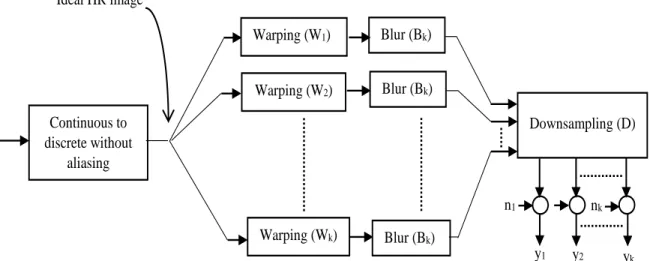
of white Gaussian noise to the HR image 𝑥, we can represent the observation model as:

𝑦𝑘 = 𝐷𝐵𝑘𝑊𝑘𝑥 + 𝑛𝑘 𝑓𝑜𝑟 𝑘 = 1 𝑡𝑜 𝐾 (3.1)

= 𝑀_𝑘𝑥 + 𝑛_𝑘

where both 𝑦_𝑘 and 𝑥 are represented in lexicographically ordered vectors having a size of 𝑀₁𝑀₂×

1 and 𝑁₁𝑁₂ × 1, respectively. 𝐷, 𝐵_𝑘, and 𝑊_𝑘 are the decimation operator, blur operator, and the

warp operator expressed in matrix form. 𝑀𝑘 is the matrix which represents all the above mentioned

degradation factors. Figure 3.2 shows a graphical representation of the observation model of Eq.

(1). Alternation in the order of blur and warp operators in the above mentioned observation model

Development Of A High Performance Mosaicing And Super-Resolution Algorithm

UND Scholarly Commons

Development Of A High Performance Mosaicing

And Super-Resolution Algorithm

TABLE OF CONTENTS

LIST OF FIGURES

LIST OF TABLES

ACKNOWLEDGEMENTS

CHAPTER 1

INTRODUCTION

CHAPTER 2

STATE-OF-THE-ART OF IMAGE MOSAICING METHODS









CHAPTER 3

STATE-OF-THE-ART OF IMAGE SUPER-RESOLUTION METHODS