Learning Transferable Representations for Visual Recognition

(1)

University of Central Florida University of Central Florida

STARS

Electronic Theses and Dissertations, 2020-

2020

Learning Transferable Representations for Visual Recognition

Yang Zhang

University of Central Florida

Part of the Computer Sciences Commons

Find similar works at: https://stars.library.ucf.edu/etd2020 University of Central Florida Libraries http://library.ucf.edu

This Doctoral Dissertation (Open Access) is brought to you for free and open access by STARS. It has been accepted for inclusion in Electronic Theses and Dissertations, 2020- by an authorized administrator of STARS. For more information, please contact [email protected].

STARS Citation STARS Citation

Zhang, Yang, "Learning Transferable Representations for Visual Recognition" (2020). Electronic Theses and Dissertations, 2020-. 162.

(2)

LEARNING TRANSFERABLE REPRESENTATIONS FOR VISUAL RECOGNITION

by

YANG ZHANG

M.S. University of Central Florida, 2016

A dissertation submitted in partial fulfilment of the requirements for the degree of Doctor of Philosophy

in the Department of Computer Science in the College of Engineering and Computer Science

at the University of Central Florida Orlando, Florida

Spring Term 2020

(3)

c

(4)

ABSTRACT

In the last half-decade, a new renaissance of machine learning originates from the applications of convolutional neural networks to visual recognition tasks. It is believed that a combination of big curated data and novel deep learning techniques can lead to unprecedented results. However, the increasingly large training data is still a drop in the ocean compared with scenarios in the wild. In this literature, we focus on learning transferable representation in the neural networks to ensure the models stay robust, even given different data distributions. We present three exemplar topics in three chapters, respectively: zero-shot learning, domain adaptation, and generalizable adversarial attack. By zero-shot learning, we enable models to predict labels not seen in the training phase. By domain adaptation, we improve a model’s performance on the target domain by mitigating its discrepancy from a labeled source model, without any target annotation. Finally, the generalization adversarial attack focuses on learning an adversarial camouflage that ideally would work in every possible scenario. Despite sharing the same transfer learning philosophy, each of the proposed topics poses a unique challenge requiring a unique solution. In each chapter, we introduce the problem as well as present our solution to the problem. We also discuss some other researchers’ approaches and compare our solution to theirs in the experiments.

(5)

LIST OF FIGURES

3.1 Given an image, its relevant tags’ word vectors rank ahead of the irrelevant

tags’ along some direction in the word vector space. We call that direction the

principal directionfor the image. To solve the problem of image tagging,

we thus learn a functionf(·)to approximate the principal direction from an

image. This function takes as the input an imagexm and outputs a vector

f(xm)for defining the principal direction in the word vector space. . . 10

3.2 Visualization of the offsets between relevant tags’ word vectors and irrelevant

ones’. Note that each vector from the origin to a point is an offset between

two word vectors.The relevant tags are shown beside the images [39]. . . 14

3.3 The existence (left) and generalization (right) of the principal direction for

each visual association rule in words induced by an image. . . 17

3.4 The neural network used in our approach for implementing the mapping

func-tionf(x;θ)from the input image, which is represented by the CNN features

x, to its corresponding principal direction in the word vector space. . . 21

3.5 The top five tags for exemplar images [39] returned by Fast0Tag on the

con-ventional, zero-shot, and seen/unseen image tagging tasks, and by TagProp

for conventional tagging. (Correct tags:green; mistaken tags: redanditalic.

(11)

3.6 The top five tags for exemplar images in [39](a) and [79](b) returned by

Fast0Tag on the conventional, zero-shot, seen/unseen and 4,093 zero-shot

image tagging tasks, and by TagProp for conventional tagging. (Correct tags:

green; mistaken tags: redanditalic) . . . 34

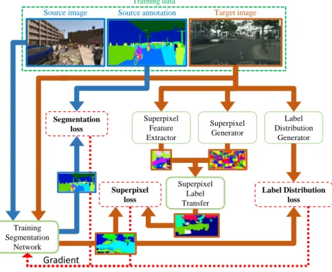
4.1 The overall framework of our curriculum domain adaptation approach to the

semantic segmentation of urban scenes. . . 47

4.2 Predictions by the same FCN-8s model, without domain adaptation, before

and after we calibrate the image’s colors. . . 48

4.3 Qualitative semantic segmentation results on the Cityscapes dataset [158]

(target domain). For each target image in the first column, we retrieve its

nearest neighbor from the SYNTHIA [40] dataset (source domain). The third

column plots the label distributions due to the groundtruth pixel-wise seman-tic annotation, the predictions by the baseline network with no adaptation, and the inferred distribution by logistic regression. The last three columns are the segmentation results by the baseline network, our domain adaptation

(12)

4.4 Qualitative semantic segmentation results on the Cityscapes dataset [158] (target domain). For each target image in the first column, we retrieve its

nearest neighbor from the GTA [156] dataset (source domain). The third

column plots the label distributions due to the groundtruth pixel-wise seman-tic annotation, the predictions by the baseline network with no adaptation, and the inferred distribution by logistic regression. The last three columns are the segmentation results by the baseline network, our domain adaptation

approach, and human annotators, respectively. . . 51

4.5 Confusion matrices for the baseline of no adaptation (left) andOurs (CC+I+SP)

(right) for the experiments of SYNTHIA-to-Cityscapes (SYNTHIA2Cityscapes,

top) and GTA-to-Cityscapes (GTA2Cityscapes, bottom). . . 62

4.6 Some “train” and “bus” images from the Cityscapes and GTA datasets. We

can see that the Cityscapes “trains” are visually more similar to the GTA

“buses” than to the GTA “trains”. . . 63

4.7 We evaluate how many superpixels are accurate in the top x% confidently

predicted superpixels. The experiments are conducted on the validation set

of Cityscapes with color constancy. . . 66

4.8 Pairwise comparison between different domain adaptation methods for the

semantic segmentation task. The entry (i, j) of this table is the number of

classes by which thei-th method outperforms thej-th. The results are

(13)

5.1 A Toyota Camry XLE in the center of the image fools the Mask R-CNN object detector after we apply the learned camouflage to it (on the right), whereas neither plain colors (on the left) nor a random camouflage (in the

middle) is able to escape the Camry from being detected. . . 79

5.2 Example procedure of a transformationt. From left to right: a16×16

cam-ouflage, a high-fidelity vehicle, a location in our simulated environment, and

an image due to this transformation over the camouflage. . . 82

5.3 The camera setup as well as some exemplar locations. The cameras depicted

in the green color are used to learn the camouflage while those in red are

unseen cameras used for testing the camouflage’s generalization. (H: camera

height,L: vehicle-to-camera distance.) . . . 83

5.4 Overview of our optimization pipeline and the clone networkVθ(c, t). . . 86

5.5 The two environments we built to learn and test the vehicle camouflage.

Zoom in for more details. These images are of the higher resolution but the same rendering quality (anti-aliasing level, shadow quality, rendering

dis-tance, texture resolution etc.) the detector perceived. . . 88

5.6 A fraction of different Toyota sedan appearances in MS COCO dataset. Their

appearances are diverse. . . 90

5.7 Orthogonal views of the Toyota Carmy XLE 2015 (second row) and the

(14)

5.8 The mIoU and [email protected] the 800 random camouflages in different resolutions on Camry in the DownTown environment. There are 100 camouflages per

resolution. . . 93

5.9 Visualization of three random camouflages of resolutions4×4,16×16, and

256×256, respectively, as well as the resulting images by the same camera. . 93

5.10 Clone network’s learned camouflage’s classification score and mIoU vs.

Sim-ulation called. We can see how the new samples helped the clone network to find the minimal. . . 100

5.11 The best detections in each image and the gradient heatmap of their

clas-sification scores w.r.t. the input images. The detector places its attention predominantly on the upper car body, i.e., roof, hood, trunk, and windows. . . 102

5.12 Qualitative comparison of the Mask R-CNN detections results of the grey

baseline color, random camouflages and our learned camouflages in different transformations. Zoom in for more details. . . 104

(15)

LIST OF TABLES

3.1 Comparison results of theconventionalimage tagging with 81 tags on

NUS-WIDE. . . 26

3.2 Comparison results of the zero-shot and seen/unseen image tagging tasks

with 81 unseen tags and 925 seen tags. . . 26

3.3 Annotating images with up to 4,093 unseen tags. . . 29

3.4 Comparison results of the conventional image tagging with 291 tags on

IAPRTC-12. . . 32

3.5 Comparison results of the zero-shot and seen/unseen image tagging tasks

with 58 unseen tags and 233 seen tags on IAPRTC-12. . . 32

4.1 χ2 _{distances between the groundtruth label distributions and those predicted}

by different methods for the adaptation from SYNTHIA to Cityscapes. . . 55

4.2 Comparison results for adapting the FCN-8s model from SYNTHIA to Cityscapes. 58

4.3 Comparison results for adapting the FCN-8s model from GTA to Cityscapes. 58

4.4 Results for the adaptation of FCN-8s from GTA to Cityscapes when we use

handcrafted features instead of the CNN features. . . 63

4.5 Results for the adaptation of FCN-8s from GTA to Cityscapes when we

use different numbers of superpixels per image. Here the images are

(16)

4.6 Results for the adaptation of ADEMXAPP [199] from GTA to Cityscapes. The ADEMXAPP net is a more powerful semantic segmentation network

than FCN-8s. . . 67

4.7 IoUs after mixing different percentages of Cityscapes images into the

SYN-THIA training dataset (SYN+CS), and of models trained with different

per-centages of Cityscapes images without any SYNTHIA images (CS only). . . 68

4.8 Comparison with the recent works published after the conference version of

our approach [210]. . . 75

5.1 Mask R-CNN detection performance on the Camry in the urban environment. 94

5.2 Detection performance of camouflages on SUV in urban environment. . . 95

5.3 YOLOv3-SPP detection performance on the Camry in the urban

environ-ment. In addition to the camouflage inferred for YOLO, we also include the

YOLO detection results on the camouflage learned for Mask R-CNN. . . 96

5.4 Detection performance of camouflages on Camry in Landscape environment.

Note that this camouflage is pretrained in urban environment and then

trans-ferred without any finetuning. . . 97

5.5 Camouflage transferability across vehicle reported in testing [email protected] urban

environment. . . 98

5.6 Detection performance of pretrained camouflages on Camry with urban

(17)

CHAPTER 1: INTRODUCTION

Transfer learning focuses on applying learned knowledge on a different and yet related problem. It has been accompanying machine learning for a long time. Some topics of transfer learning include domain adaptation, transductive learning, zero-shot learning, and semi-supervised learning, etc. Transfer learning has been an active research field before the rise of deep learning.

However, it was not until neural network regained attention [99] did researchers realize there are

ample new opportunities. The neural networks bring two new challenges to the table for transfer learning: feature learning and complex tasks. One of the main reasons that neural networks

be-ing popular is their learnbe-ing powerful and transferable intermediate features [205] directly from

high dimension raw input. The capability of learning representations from raw data encourages researchers to take advantage of the feature learning of the neural networks in transfer learning.

Take domain adaptation as an example. Previous shallow domain adaptation [143] aims to adapt

machine learning models with given features. In contrast, recent deep domain adaptation [65]

con-centrates on learning CNN as an invariant feature extractor with raw input. How will we train a neural network as a high-performing and robust feature extractor?

Secondly, increasing neural network capability benefits many structured prediction tasks in an end-to-end style. For example, object detection used to need a dedicated complex model such

as DPM [53] and a considerable amount of tricks to train the model. Nowadays, one

Mask-RCNN [81] is sufficient. Such advancement paves the way for studying previously difficult tasks

in the scope of transfer learning. For instance, domain adaptation for segmentation [86,210]

fol-lowed FCN [114]. However, the more complex the tasks become, the harder it is to disentangle

features in transfer learning. How can we disentangle the features in complex tasks and networks?

(18)

deep learning has fundamentally changed different transfer learning problems and how we can use deep learning as a tool to address the previous two questions.

We first describe zero-shot image tagging in chapter 3. Zero-shot learning trains a model to predict labels that are unseen during the training phase. It is common to transfer knowledge of known training labels to unseen labels via their semantically encoded word vectors. However, unlike commonly studied zero-shot image classification, we want to study a more general image tagging scenario, where each image may possess multiple labels. We begin by looking into a particular image-word relation in this chapter. Our results show that the word vectors of relevant tags for a given image rank ahead of the irrelevant tags, along a principal direction in the word vector space. Inspired by this observation, we propose to solve image tagging by estimating the principal direction for an image. Particularly, we exploit linear mappings and nonlinear deep neural networks to approximate the principal direction from an input image. We arrive at a quite versatile tagging model. It runs fast given a test image, in constant time w.r.t. the training set size. It not only yields superior performance for the conventional tagging task on the NUS-WIDE dataset, but also

outperforms competitive baselines on annotating images with previouslyunseentags.

In chapter 4, we describe domain adaptation for semantic segmentation and our solution to it. Training semantic segmentation CNNs requires a considerable amount of data, which is difficult to collect and laborious to annotate. Recent advances in computer graphics make it possible to train CNNs on photo-realistic synthetic imagery with computer-generated annotations. Despite this, the domain mismatch between real images and the synthetic data hinders the models’ performance. Hence, we propose a curriculum-style learning approach to minimizing the domain gap in urban scene semantic segmentation. The curriculum domain adaptation solves easy tasks first to infer necessary properties about the target domain; in particular, the first task is to learn global label distributions over images and local distributions over landmark superpixels. These are easy to estimate because images of urban scenes have strong idiosyncrasies (e.g., the size and spatial

(19)

relations of buildings, streets, cars, etc.). We then train a segmentation network, while regularizing its predictions in the target domain to follow those inferred properties. In experiments, our method outperforms the baselines on two datasets and three backbone networks. We also report extensive ablation studies about our approach.

Lastly, in chapter 5, we conduct an intriguing experimental study about a generalizable physical adversarial attack on object detectors in the wild. In particular, we learn a camouflage pattern to hide vehicles from being detected by state-of-the-art convolutional neural network based detectors. Our approach alternates between two threads. In the first, we train a neural approximation function to imitate how a simulator applies a camouflage to vehicles and how a vehicle detector performs given images of the camouflaged vehicles. In the second, we minimize the approximated detection score by searching for the optimal camouflage. Experiments show that the learned camouflage can not only hide a vehicle from the image-based detectors under many test cases but also generalizes to different environments, vehicles, and object detectors.

(20)

CHAPTER 2: LITERATURE REVIEW

2.1 Image Tagging

Image tagging aims to assign relevant tags to an image or to return a ranking list of tags. In the liter-ature this problem has been mainly approached from the tag ranking perspective. In the generative

methods, which involve topic models [17,125,204,133] and mixture models [104,93,182,54,29,

46], the candidate tags are naturally ranked according to their probabilities conditioned on the test

image. For the non-parametric nearest neighbor based methods [120,121,108,95,80, 107, 214],

the tags for the test image are often ranked by the votes from some training images. The nearest

neighbor based algorithms, in general, outperform those depending on generative models [95,109],

but suffer from high computation costs in both training and testing. The recent FastTag

algo-rithm [34] is magnitude faster and achieves comparable results with the nearest neighbor based

methods. The embedding method [196] assigns ranking scores to the tags by a cross-modality

mapping between images and tags. This idea is further exploited using deep neural networks [75].

Interestingly, none of these methods learn their models explicitly for the ranking purpose

ex-cept [196, 75], although they all rank the candidate tags for the test images. Thus, there exists

a mismatch between the models learned and the actual usage of the models, violating the principle of Occam’s razor.

2.2 Word Embedding

Instead of representing words using the traditional one-hot vectors, word embedding maps each word to a continuous-valued vector, by learning from primarily the statistics of word co-occurrences.

(21)

on the most recent GloVe [148] and word2vec vectors [124,123,122]. As shown in the well-known

word analogy experiments [124, 148], both types of word vectors are able to capture fine-grained

semantic and syntactic regularities using vector offsets.

2.3 Zero-shot Learning

Zero-shot learning is often used exchange-ably with zero-shot classification, whereas the latter is a

special case of the former. Unlike weakly-supervised learning [128,59] which learn new concepts

by mining noisy new samples, zero-shot classification learns classifiers from seen classes and aims

to classify the objects of unseen classes [136,135,103,6,60,92,135,136,177]. Attributes [102,

52] and word vectors are two of the main semantic sources making zero-shot classification feasible.

Our Fast0Tag along with [61] enriches the family of zero-shot learning by zero-shot multi-label

classification [189]. Fu et al. [61] reduce the problem to zero-shot classification by treating every

combination of the multiple labels as a class. We instead directly model the labels and are able to assign/rank many unseen tags for an image.

2.4 Domain adaptation

Conventional machine learning algorithms rely on the standard assumption that the training and test data are drawn i.i.d. from the same underlying distribution. However, it is often the case that there exists some discrepancy between the training and test stages. Domain adaptation aims to

rectify this mismatch and tune the models toward better generalization at the test stage [186, 185,

73,97,78].

(22)

prob-lems [143, 138], e.g., learning from online images to classify real world objects [163, 74], and,

more recently, aims to improve the adaptability of deep neural networks [115, 66, 65, 190, 22].

Among them, the most relevant works to ours are those exploring simulated data [179, 203, 158,

194, 86, 146, 172]. Sun and Saenko train generic object detectors from synthetic images [179],

while Vazquez et al. use virtual images to improve pedestrian detections in real environments [194].

The other way around, i.e., how to improve the quality of the simulated images using the real ones,

is studied in [172,146].

2.5 Semantic Segmentation

Semantic segmentation is the task of assigning an object label to each pixel of an image. Traditional

methods [171,184,208] rely on local image features manually designed by domain experts. After

the pioneering works [32, 114] that introduced the convolutional neural network (CNN) [106] to

semantic segmentation, most recent top-performing methods are also built on CNNs [199,160,15,

212,134,44].

Currently, there are multiple and increasing numbers of semantic segmentation datasets aiming for different computer vision applications. Some general ones include the PASCAL VOC2012

Chal-lenge [48], which contains nearly 10,000 annotated images for the segmentation competition, and

the MS COCO Challenge [111], which includes over 200,000 annotated images. In our paper, we

focus on urban outdoor scenes. Several urban scene segmentation datasets are publicly available

such as Cityscapes [40], a vehicle-centric dataset created primarily in German cities, KITTI [68],

another vehicle-centric dataset captured in the German city Karlsruhe, Berkeley DeepDrive Video

Dataset [202], a dashcam dataset collected in United States, Mapillary Vistas Dataset [131], so far

known as the largest outdoor urban scene segmentation dataset collected from all over the world,

(23)

and low-resolution toy dashcam dataset. An enormous amount of labor-intensive work is required

to annotate the images that are needed to obtain accurate segmentation models. According to [156],

it took about 60 minutes to manually segment each image in [23] and about 90 minutes for each

in [40]. A plausible approach to reducing the human annotation workload is to utilize weakly

supervised information such as image labels and bounding boxes [144,87,140,151].

We instead explore the almost labor-free labeled virtual images for training high-quality

segmen-tation networks. In [156], annotating a synthetic image took only 7 seconds on average through a

computer game. For the urban scenes, we use the SYNTHIA [158] and GTA [156] datasets which

contain images of virtual cities. Although not used in our experiments, another synthetic

seg-mentation dataset worth mentioning is Virtual KITTI [62], a synthetic duplication of the original

KITTI [68] dataset.

2.6 Domain Adaptation for Semantic Segmentation

Due to the clear visual mismatch between synthetic and real data [169,156,158], we expect to use

domain adaptation to enhance the segmentation performance on real images by networks trained

on synthetic imagery. To the best of our knowledge, our work [210] and the FCNs in the wild [86]

are among the very first attempts to tackle this problem. It subsequently became an independent

track in the Visual Domain Adaptation Challenge (VisDA) 2017 [147]. After that, some

feature-alignment based methods were developed [167,85,165,37,198]. We postpone further discussion

to Section 4.4, which presents a comprehensive survey of the works published after ours and before December 2018. We group them into two major categories and describe their main methods. We also summarize their results in Table 4.8 and analyze their complementary relationships with ours.

(24)

2.7 Adversarial Attack and its Generalization

Currently, the adversarial attack is powerful enough to attack image classification [126], object

detection [11], semantic segmentation [201], audio recognition [28] and even bypass most of the

defense mechanism [12]. The mainstream adversarial machine learning research focuses on the

in silico ones or the generalization within in silico [113]. Such learned perturbations are

practi-cally unusable in the real world as shown in the experiments by [118], who found that almost all

perturbation methods failed to prevent a detector from detecting real stop signs.

The first physical world adversarial attack by [101] found perturbations remain effective on the

printed paper. [51] found a way to train perturbations that remain effective against a classifier

on real stop signs for different viewing angles and such. [13] trained another perturbation that

successfully attacks an image classifier on 3D-printed objects. However [119] found that [51]’s

perturbation does not fool the object detectors YOLO9000 [152] and Faster RCNN [154]. They

argue that fooling an image classifier is different and easier than fooling an object detector

be-cause the detector is able to propose object bounding boxes on its own. In the meanwhile, [117]’s

and [36]’s work could be generalized to attack the stop sign detector in the physical world more

effectively. However, all the above methods aim to perturb detecting the stop signs.

Blackbox attack is another relevant topic. Among the current blackbox attack literature, [141]

trained a target model substitution based on the assumption that the gradient between the image and the perturbation is available. We do not have the gradient since the simulation is nondifferentiable.

[35] proposed a coordinate descent to attack the model. However, we found that our optimization

problem is time-consuming, noisy , empirically non-linear and non-convex. Time constraints made this approach unavailable to us since it requires extensive evaluations during coordinate descent. Besides, coordinate descent generally requires precise evaluation at each data-point.

(25)

2.8 Simulation aided Machine Learning

Since the dawn of deep learning, data collection has always been of fundamental importance as deep learning model performance is generally correlated with the amount of training data used. Given the sometimes unrealistically expensive annotation costs, some machine learning researchers use synthetic data to train their models. This is especially true in computer vision

ap-plications since state-of-the-art computer-generated graphics are truly photo-realistic. [159, 155]

proposed synthetic datasets for semantic segmentation. [63] proposed virtual KITTI as a synthetic

replica of the famous KITTI dataset [69] for tracking, segmentation, etc. And [193] proposed

us-ing synthetic data for human action learnus-ing. [209, 21] adapt RL-trained robot grasping models

from the synthetic environment to the real environment. [187] trained a detection network using

(26)

CHAPTER 3: ZERO SHOT IMAGE TAGGING

3.1 Problem Introduction

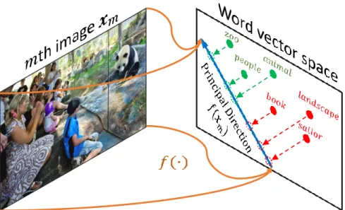
Figure 3.1: Given an image, its relevant tags’ word vectors rank ahead of the irrelevant tags’ along

some direction in the word vector space. We call that direction the principal direction for the

image. To solve the problem of image tagging, we thus learn a function f(·)to approximate the

principal direction from an image. This function takes as the input an image xm and outputs a

vectorf(xm)for defining the principal direction in the word vector space.

Recent advances in the vector-space representations of words [122,123,148] have benefited both

NLP [176, 216, 183] and computer vision tasks such as zeros-shot learning [177,58, 6] and

im-age captioning [105, 96, 98]. The use of word vectors in NLP is grounded on the fact that the

This chapter contains previously published materials from “Fast zero-shot image tagging” by Yang Zhang, Bo-qing Gong, and Mubarak Shah, published in Proceedings of the IEEE Conference on Computer Vision and Pattern Recognition in 2016.

(27)

fine-grainedlinguistic regularities over words are captured by linear word vector offsets—a key

observation from the well-known word analogy experiments [124, 148], such as the syntactic

re-lationdance−dancing ≈f ly−f lyingand semantic relationking−man≈queen−woman.

However, it is unclear whether thevisualregularities over words, which are implicitly used in the

aforementioned computer vision problems, can still be encoded by the simple vector offsets.

In this chapter, we are interested in the problem of image tagging, where an image (e.g., of a zoo in Figure 3.1) calls for a partition of a vocabulary of words into two disjoint sets according

to the image-word relevance (e.g., relevant tags Y = {people, animal, zoo} and irrelevant ones

Y = {sailor, book, landscape}). This partitioning of words,(Y, Y), is essentially different from the fine-grained syntactic (e.g., dance to dancing) or semantic (e.g., king to man) relation tested in the word analogy experiments. Instead, it is about the relationship between two sets of words

due to a visual image. Such a relation in words is semantic and descriptive, and focuses onvisual

association, albeit relatively coarser. In this case, do the word vectors still offer the nice property, that the simple linear vector offsets can depict the visual (image) association relations in words?

For the example of the zoo, while humans are capable of easily answering that the words inY are

more related to the zoo than those inY, can such zoo-association relation in words be expressed

by the 9 pairwise word vector offsets {people−sailor, people− book,· · · , zoo− landscape}

between the relevantY and irrelevantY tags’ vectors?

One of the main contributions of this chapter is to empirically examine the above two questions

(cf. Section 3.2). Every image introduces a visual association rule(Y, Y)over words. Thanks to

the large number of images in benchmark datasets for image tagging, we are able to examine many

distinctvisual association regulations in words and the corresponding vector offsetsin the word

vector space. Our results reveal a somehow surprising connection between the two: the offsets

between the vectors of the relevant tagsY and those of the irrelevantY are along about the same

(28)

vector offsets. In other words, there exists at least one vector (direction) w in the word vector

space, such that its inner products with the vector offsets betweenY andY are greater than 0, i.e.,

∀p∈Y,∀n∈Y,

hw,p−ni>0equivalently, hw,pi>hw,ni, (3.1)

where the latter reads that the vectorw ranksall relevant wordsY (e.g., for the zoo image) ahead

of the irrelevant onesY. For brevity, we overload the notationsY andY to respectively denote the

vectors of the words in them.

The visual association relations in words thus represent themselves by the (linear) rank-abilities of the corresponding word vectors. This result reinforces the conclusion from the word anal-ogy experiments that, for a single word multiple relations are embedded in the high dimensional

space [124,148]. Furthermore, those relations can be expressed by simple linear vector arithmetic.

Inspired by the above observation, we propose to solve the image tagging problem by estimating the principal direction, along which the relevant tags rank ahead of the irrelevant ones in the word vector space. Particularly, we exploit linear mappings and deep neural networks to approximate the principal direction from each input image. This is a grand new point of view to image tagging and results in a quite versatile tagging model. It operates fast given a test image, in constant time with respect to the training set size. It not only gives superior performance for the conventional tagging task, but is also capable of assigning novel tags from an open vocabulary, which are unseen

at the training stage. We do not assume anya priori knowledge about these unseen tags as long

as they are in the same vector space as the seen tags for training. To this end, we name our

approach fast zero-shot image tagging (Fast0Tag) to recognize that it possesses the advantages of

(29)

In sharp contrast to our approach, previous image tagging methods can only annotate test images

with the tags seen at training except [61], to the best of our knowledge. Limited by the static and

usually small number of seen tags in the training data, these models are frequently challenged in practice. For instance, there are about 53M tags on Flickr and the number is rapidly growing.

The work of [61] is perhaps the first attempt to generalize an image tagging model to unseen tags.

Compared to the proposed method, it depends on two extra assumptions. One is that the unseen

tags are knowna prioriin order to tune the model towards their combinations. The other is that the

test images are knowna priori, to regularize the model. Furthermore, the generalization of [61]

is limited to a very small number, U, of unseen tags, as it has to consider all the 2U _possible

combinations.

To summarize, our first main contribution is on the analyses of the visual association relations in words due to images, and how they are captured by word vector offsets. We hypothesize and

empirically verify that, for each visual association rule(Y, Y), in the word vector space there exists

a principal direction, along which the relevant words’ vectors rank ahead of the others’. Built upon

this finding, the second contribution is a novel image tagging model, Fast0Tag, which is fast and

generalizes to open-vocabulary unseen tags. Last but not least, we explore three different image

tagging scenarios: conventional tagging which assigns seen tags to images, zero-shot tagging

which annotates images by (a large number of) unseen tags, andseen/unseentagging which tags

images with both seen and unseen tags. In contrast, the existing work tackles either conventional

tagging, or zero-shot tagging with very few unseen tags. Our Fast0Tag gives superior results over

(30)

green, wildlife, spring, desert, Nevada bike, bicycle, glow, sunlight, light, people, summer, august, France, Paris, silhouette, mist, silhouettes, olympus, blue t-SNE visualization of word vector offsets.

Origin Principal direction Principal direction PCA visualization of word vector offsets.

Origin Principal direction Origin Principal direction Origin

Figure 3.2: Visualization of the offsets between relevant tags’ word vectors and irrelevant ones’.

Note that each vector from the origin to a point is an offset between two word vectors.The relevant

tags are shown beside the images [39].

3.2 The linear rank-ability of word vectors

Our Fast0Tag approach benefits from the finding that the visual association relation in words, i.e.,

the partition of a vocabulary of words according to their relevances to an image, expresses itself in the word vector space as the existence of a principal direction, along which the words/tags relevant to the image rank ahead of the irrelevant ones. This section details the finding.

3.2.1 The regulation over words due to image tagging

We useSto denote the seen tags available for training image tagging models andU the tags unseen

at the training stage. The training data are in the form of {(xm, Ym);m = 1,2,· · ·,M}, where

xm ∈ RD is the feature representation of imagem andYm ⊂ S are the seen tags relevant to that

(31)

word/tag vectors.

Theconventionalimage tagging aims to assign seen tags in S to the test images. The zero-shot

tagging, formalized in [61], tries to annotate test images using a pre-fixed set of unseen tags U.

In addition to those two scenarios, this chapter considersseen/unseenimage tagging, which finds

both relevant seen tags fromS and relevant unseen tags fromU for the test images. Furthermore,

the set of unseen tagsU could be open and dynamically growing.

Denote by Ym := L \Ym the irrelevant seen tags. An image m introduces a visual association

regulation to words—the partition (Ym, Ym) of the seen tags to two disjoint sets. Noting that

many fine-grained syntactic and semantic regulations over words can be expressed by linear word vector offsets, we next examine what properties the vector offsets could offer for this new visual association rule.

3.2.2 Principal direction and cluster structure

Figure 3.2 visualizes the vector offsets(p−n),∀p∈ Ym,∀n ∈Ym using t-SNE [192] and PCA

for two visual association rules over words. One is imposed by an image with5relevant tags and

the other is with15relevant tags. We observe two main structures from the vector offsets:

Principal direction. Mostly, the vector offsets point to about the same direction (relative to the

origin), which we call the principal direction, for a given visual association rule(Ym, Ym)in

words for imagem. This implies that the relevant tagsYm rank ahead of the irrelevant ones

Ym along the principal direction (cf. eq. (3.1)).

Cluster structure. There exist cluster structures in the vector offsets for each visual association

(32)

fall into the same cluster. We differentiate the offsets pointing to different relevant tags by colors in Figure 3.2.

Can the above two observations generalize? Namely, do they still hold in the high-dimensional word vector space for more visual association rules imposed by other images? To answer the questions, we next design an experiment to verify the existence of the principal directions in word vector spaces, or equivalently the linear rank-ability of word vectors. We leave the cluster structure for future research.

3.2.3 Testing the linear rank-ability hypothesis

Our experiments in this section are conducted on the validation set (26,844 images, 925 seen tags

S, and 81 unseen tagsU) of NUS-WIDE [39]. The number of relevant seen/unseen tags associated

with an image ranges from 1 to 20/117 and on average is 1.7/4.9. See Section 3.4 for details.

Our objective is to investigate, for any visual association rule(Ym, Ym)in words by imagem, the

existence of the principal direction along which the relevant tagsYm rank ahead of the irrelevant

tagsYm. The proof completes once we find a vectorw in the word vector space that satisfies the

ranking constraintshw,pi > hw,ni,∀p∈ Ym,∀n ∈ Ym. To this end, we train a linear ranking

SVM [94] for each visual association rule using all the corresponding pairs(p,n), then rank the

word vectors by the SVM, and finally examine how many constraints are violated. In particular, we employ MiAP, the larger the better (cf. Section 3.4), to compare the SVM’s ranking list with those ranking constraints. We repeat the above process for all the validation images, resulting in 21,863 unique visual association rules.

(33)

SVM in the primal [30] with the following formulation: min w λ 2kwk 2 + X yi∈Ym X yj∈Ym max(0,1−wyi+wyj)

whereλis the hyper-parameter controlling the trade-off between the objective and the

regulariza-tion. 1 4 16 64 256 70% 75% 80% 85% 90% 95% 100% λ MiAP 1 4 16 64 256 0% 10% 20% 30% 40% λ MiAP Glove 300D Word2vec 100D Word2vec 300D Word2vec 500D Word2vec 1000D Random

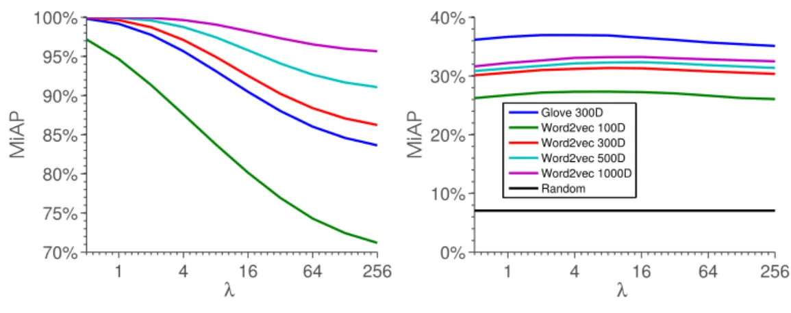
Figure 3.3: The existence (left) and generalization (right) of the principal direction for each visual association rule in words induced by an image.

Results.The MiAP results averaged over all the distinct regulations are reported in Figure 3.3(left),

in which we test the 300D GloVe vectors [148] and word2vec [124] of dimensions 100, 300, 500,

and 1000. The horizontal axis shows different regularizations we use for training the ranking

SVMs. Largerλregularizes the models more. In the 300D GloVe space and the word2vec spaces

of 300, 500, and 1000 dimensions, more than two ranking SVMs, with small λ values, give rise

to nearly perfect ranking results (MiAP ≈ 1), showing that the seen tagsL are linearly rank-able

under almost every visual association rule—all the ranking constraints imposed by the relevantYm

and irrelevantYmtags to imagemare satisfied.

(34)

Lof seen tags. An imagemincurs a visual association rule essentially over all words, though the

same rule implies different partitions of distinct experimental vocabularies (e.g., the seen tags L

and unseen onesU). Accordingly, we would expect the principal direction for the seen tags is also

shared by the unseen tags under the same rule, if the answer is YES to the questions at the end of Section 3.2.2.

Generalization to unseen tags. We test whether the same principal direction exists for the seen tags and unseen ones under every visual association rule induced by an image. This can be (only partially) justified by applying the ranking SVMs previously learned, to the unseen tags’ vectors, because we do not know the “true” principal directions. We consider the with 81 unseen tags

U as the “test data” for the trained ranking SVMs, each due to an image incurred visual

associ-ation. NUS-WIDE provides the annotations of the 81 tags for the images. The results, shown in Figure 3.3(right), are significantly better than the most basic baseline, randomly ranking the tags (the black curve close to the origin), demonstrating that the directions output by SVMs are

generalizable to the new vocabularyU of words.

Observation. Therefore, we conclude that the word vectors are an efficient media to transfer knowledge—the rank-ability along the principal direction—from the seen tags to the unseen ones.

We have empirically verified that the visual association rule(Ym, Ym)in words due to an imagem

can be represented by the linear rank-ability of the corresponding word vectors along a principal

direction. Our experiments involve|L|+|U |=1,006 words in total. Larger-scale and theoretical

(35)

3.3 Approximating the linear ranking functions

This section presents our Fast0Tag approach to image tagging. We first describe how to solve image

tagging by approximating the principal directions thanks to their existence and generalization, empirically verified in the last section. We then describe detailed approximation techniques.

3.3.1 Image tagging by ranking

Grounded on the observation from Section 3.2, that there exists a principal direction wm, in the

word vector space, for every visual association rule(Ym, Ym)in words by an imagem, we propose

a straightforward solution to image tagging. The main idea is to approximate the principal direction

by learning a mapping functionf(·), between the visual space and the word vector space, such that

f(xm)≈wm, (3.2)

wherexm is the visual feature representation of the imagem. Therefore, given a test imagex, we

can immediately suggest a list of tags by ranking the word vectors of the tags along the direction

f(x), namely, by the ranking scores,

hf(x),ti, ∀t ∈ L ∪ U (3.3)

no matter the tags are from the seen setS or unseen setU.

We explore both linear and nonlinear neural networks for implementing the approximation function

(36)

3.3.2 Approximation by linear regression

Here we assume a linear function from the input image representation x to the output principal

directionw, i.e.,

f(x) :=Ax, (3.4)

whereAcan be solved in a closed form by linear regression. Accordingly, we have the following

from the training

wm =Axm+m, m= 1,2,· · · ,M (3.5)

wherewm is the principal direction of all offset vectors of the seen tags, for the visual association

rule (Ym, Ym) due to the image m, and m are the errors. Minimizing the mean squared errors

gives us a closed form solution toA.

One caveat is that we do not know the exact principal directionswmat all—the training data only

offer imagesxmand the relevant tagsYm. Here we take the easy alternative and use the directions

found by ranking SVMs (cf. Section 3.2) in eq. (3.5). There are thustwo stagesinvolved to learn

the linear functionf(x) =Ax. The first stage trains a ranking SVM over the word vectors of seen

tags for each visual association(Ym, Ym). The second stage solves for the mapping matrix Aby

linear regression, in which the targets are the directions returned by the ranking SVMs.

Discussion. We note that the the linear transformation between visual and word vector spaces has

been employed before, e.g., for zero-shot classification [6,58] and image annotation/classification [197].

This work differs from them with a prominent feature, that the mapped imagef(x) = Axhas a

(37)

to be assigned to the image. We next extend the linear transformation to a nonlinear one, through a neural network. D rop ou t 30% D en se R e lu

𝑓(∙)

𝒙

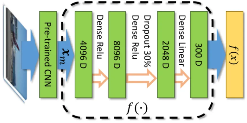
𝑚 4096 D 2048 D D en se Line ar Pr e-tr aine d CNN 300 D 𝑓(𝑥) D en se R e lu 8096 D

Figure 3.4: The neural network used in our approach for implementing the mapping function

f(x;θ) from the input image, which is represented by the CNN featuresx, to its corresponding

principal direction in the word vector space.

3.3.3 Approximation by neural networks

We also exploit a nonlinear mappingf(x;θ)by a multi-layer neural network, whereθdenotes the

network parameters. Figure 3.4 shows the network architecture. It consists of two RELU layers

followed by a linear layer to output the approximated principal direction, w, for an input image

x. We expect the nonlinear mapping functionf(x;θ)to offer better modeling flexibility than the

linear one.

Can we still train the neural network by regressing to the M directions obtained from ranking

SVMs? Both our intuition and experiments tell that this is a bad idea. The numberMof training

instances is small relative to the number of parameters in the network, making it hard to avoid overfitting. Furthermore, the directions by ranking SVMs are not the true principal directions anyway. There is no reason for us to stick to the ranking SVMs for the principal directions.

(38)

We instead unify the two stages in Section 3.3.2. Recall that we desire the output of the neural

networkf(xm;θ)to be the principal direction, along which all the relevant tag vectorsp∈Ymof

an imagemrank ahead of the irrelevant onesn∈Ym. Denote by

ν(p,n;θ) = hf(xm;θ),ni − hf(xm;θ),pi,

the amount of violation to any of those ranking constraints. We minimize the following loss to train the neural network,

θ? ←arg min_θ M X m=1 ωm`(xm, Ym;θ), (3.6) `(xm, Ym;θ) = X p∈Ym X n∈Ym log (1 + exp{ν(p,n;θ)}) whereωm = |Ym||Ym| −1

normalizes the per-image RankNet loss [27]`(xm, Ym;θ)by the

num-ber of ranking constraints imposed by the image m over the tags. This formulation enables the

function f(x)to directly take account of the ranking constraints by relevant p and irrelevantn

tags. Moreover, it can be optimized with no challenge at all by standard mini-batch gradient de-scent.

Practical considerations. We use Theano [19] to solve the optimization problem. A mini-batch consists of 1,000 images, each of which incurs on average 4,600 pairwise ranking constraints of

the tags—we use all pairwise ranking constraints in the optimization. The normalization ωm for

the per-image ranking loss suppresses the violations from the images with many positive tags. This is desirable since the numbers of relevant tags of the images are unbalanced, ranging from 1 to 20. Without the normalization the MiAP results drop by about 2% in our experiments. For

regularization, we use early stopping and a dropout layer [84] with the drop rate of 30%. The

(39)

In addition to the RankNet loss [27] in eq. (3.6), we have also experimented some other choices for

the per-image loss, including the hinge loss [41], Crammer-Singer loss [42], and pairwise max-out

ranking [94]. The hinge loss performs the worst, likely because it is essentially not designed for

ranking problems, though one can still understand it as a point-wise ranking loss. The Crammer-Singer, pairwise max-out, and RankNet are all pair-wise ranking loss functions. They give rise to comparable results and RankNet outperforms the other two by about 2% in terms of MiAP. This may attribute to the ease of control over the optimization process for RankNet. Finally, we note

that the list-wise ranking loss [200] can also be employed.

3.4 Experiments on NUS-WIDE

This section presents our experimental results. We contrast our approach to several competitive

baselines for the conventional image tagging task on the large-scale NUS-WIDE [39] dataset.

Moreover, we also evaluate our method on the zero-shot and seen/unseen image tagging problems (cf. Section 3.2.1). For the comparison on these problems, we extend some existing zero-shot classification algorithms and consider some variations of our own approach.

3.4.1 Dataset and evaluation

3.4.1.1 NUS-WIDE

We mainly use the NUS-WIDE dataset [39] for the experiments in this section. NUS-WIDE is a

standard benchmark dataset for image tagging. It contains 269,648 images in the original release and we are able to retrieve 223,821 of them since some images are either corrupted or removed from Flickr. We follow the recommended experiment protocol to split the dataset into a training set with 134,281 images and a test set with 89,603 images. We further randomly separate 20%

(40)

from the training set as our validation set for 1) tuning hyper-parameters in our method and the baselines and 2) conducting the empirical analyses in Section 3.2.

3.4.1.2 Annotations of NUS-WIDE

NUS-WIDE releases three sets of tags associated with the images. The first set comprises of 81 “groundtruth” tags. They are carefully chosen to be representative of the Flickr tags, such as

con-taining both general terms (e.g.,animal) and specific ones (e.g.,dog andf lower), corresponding

to frequent tags on Flickr, etc. Moreover, they are annotated by high-school and college students and are much less noisy than those directly collected from the Web. This 81-tag set is usually taken as the groundtruth for benchmarking different image tagging methods. The second and the third sets of annotations are both harvested from Flickr. There are 1,000 popular Flickr tags in the second set and nearly 5,000 raw tags in the third.

3.4.1.3 Image features and word vectors

We extract and`2normalize the image feature representations of VGG-19 [175]. Both GloVe [148]

and Word2vec [124] word vectors are included in our empirical analysis experiments in Section 3.2

and the 300D GloVe vectors are used for the remaining experiments. We also`2normalize the word

vectors.

3.4.2 Evaluation

We evaluate the tagging results of different methods using two types of metrics. One is the mean image average precision (MiAP), which takes the whole ranking list into account. The other

(41)

K = 3andK = 5. Both metrics are commonly used in the previous works on image tagging. We

refer the readers to Section 3.3 of [109] for how to calculate MiAP and to Section 4.2 of [75] for

the top-K precision and recall.

3.4.3 Conventional image tagging

Here we report the experiments on theconventionaltagging. The 81 concepts with “groundtruth”

annotations in NUS-WIDE are used to benchmark different methods.

3.4.3.1 Baselines

We include TagProp [80] as the first competitive baseline. It is representative among the nearest

neighbor based methods, which in general outperform the parametric methods built from

genera-tive models [17,29], and gives rise to state-of-the-art results in the experimental study [109]. We

further compare with two most recent parametric methods, WARP [75] and FastTag [34], both of

which are built upon deep architectures though using different models. For a fair comparison, we use the same VGG-19 features for all the methods—the code of TagProp and FastTag is provided by the authors and we implement WARP based on our neural network architecture. Finally, we

compare to WSABIE [197] and CCA, both correlating images and relevant tags in a low

dimen-sional space. All the hyper-parameters (e.g., the number of nearest neighbors in TagProp and early stopping for WARP) are selected using the validation set.

3.4.3.2 Results

Table 3.1 shows the comparison results of TagProp, WARP, FastTag, WSABIE, CCA, and our

(42)

Table 3.1: Comparison results of theconventionalimage tagging with 81 tags on NUS-WIDE. Method % MiAP K= 3 K= 5 P R F1 P R F1 CCA 19 9 15 11 7 20 11 WSABIE [197] 28 16 27 20 12 35 18 TagProp [80] 53 29 50 37 22 62 32 WARP [75] 48 27 45 34 20 57 30 FastTag [34] 41 23 39 29 19 54 28 Fast0Tag (lin.) 52 29 50 37 21 60 31 Fast0Tag (net.) 55 31 52 39 23 65 34

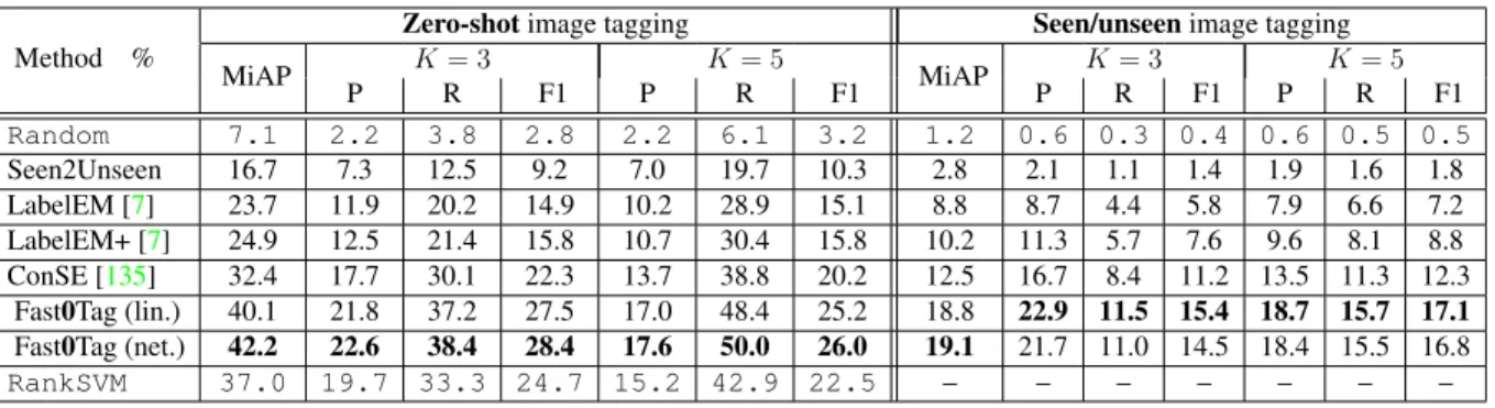
Table 3.2: Comparison results of the zero-shot and seen/unseen image tagging tasks with 81

unseen tags and 925 seen tags.

Method %

Zero-shotimage tagging Seen/unseenimage tagging

MiAP K= 3 K= 5 MiAP K= 3 K= 5 P R F1 P R F1 P R F1 P R F1 Random 7.1 2.2 3.8 2.8 2.2 6.1 3.2 1.2 0.6 0.3 0.4 0.6 0.5 0.5 Seen2Unseen 16.7 7.3 12.5 9.2 7.0 19.7 10.3 2.8 2.1 1.1 1.4 1.9 1.6 1.8 LabelEM [7] 23.7 11.9 20.2 14.9 10.2 28.9 15.1 8.8 8.7 4.4 5.8 7.9 6.6 7.2 LabelEM+ [7] 24.9 12.5 21.4 15.8 10.7 30.4 15.8 10.2 11.3 5.7 7.6 9.6 8.1 8.8 ConSE [135] 32.4 17.7 30.1 22.3 13.7 38.8 20.2 12.5 16.7 8.4 11.2 13.5 11.3 12.3

Fast0Tag (lin.) 40.1 21.8 37.2 27.5 17.0 48.4 25.2 18.8 22.9 11.5 15.4 18.7 15.7 17.1

Fast0Tag (net.) 42.2 22.6 38.4 28.4 17.6 50.0 26.0 19.1 21.7 11.0 14.5 18.4 15.5 16.8

RankSVM 37.0 19.7 33.3 24.7 15.2 42.9 22.5 – – – – – – –

We can see that TagProp performs significantly better than WARP and FastTag. However,

Tag-Prop’s training and test complexities are very high, being respectivelyO(M2₎_and_O_(M)_{w.r.t. the}

training set sizeM. In contrast, both WARP and FastTag are more efficient, with O(M)training

complexity and constant testing complexity, thanks to their parametric formulation. Our Fast0Tag

with linear mapping gives comparable results to TagProp and Fast0Tag with the neural network

outperforms the other methods. Also, both implementations have as low computation complexities as WARP and FastTag.

(43)

3.4.4 Zero-shot and Seen/Unseen image tagging

This section presents some results for the two novel image tagging scenarios, zero-shot and

seen/unseentagging.

Fu et al. [61] formalized the zero-shot image tagging problem, aiming to annotate test images

using a pre-fixed setU of unseen tags. Our Fast0Tag naturally applies to this scenario, by simply

ranking the unseen tags with eq. (3.3). Furthermore, this paper also considersseen/unseenimage

tagging which finds both relevant seen tags from S and relevant unseen tags fromU for the test

images. The set of unseen tagsU could be open and dynamically growing.

In our experiments, we treat the 81 concepts with high-quality user annotations in NUS-WIDE

as the unseen set U for evaluation and comparison. We use the remaining 925 out of the 1000

frequent Flickr tags to form the seen setS—75 tags are shared by the original 81 and 1,000 tags.

3.4.4.1 Baselines

Our Fast0Tag models can be readily applied to the zero-shot and seen/unseen image tagging

scenarios. For comparison we study the following baselines.

Seen2Unseen. We first propose a simple method which extends an arbitrary traditional image tagging method to also working with previously unseen tags. It originates from our analysis experiment in Section 3.2. First, we use any existing method to rank the seen tags for a test image. Second, we train a ranking SVM in the word vector space using the ranking list of the seen tags. Third, we rank unseen (and seen) tags using the learned SVM for zero-shot (and seen/unseen) tagging.

(44)

for fine-grained object recognition. If we consider each tag ofS ∪U as a unique class, though this implies that some classes will have duplicated images, the LabelEM can be directly applied to the two new tagging scenarios.

LabelEM+. We also modify the objective loss function of LabelEM when we train the model, by carefully removing the terms that involve duplicated images. This slightly improves the performance of LabelEM.

ConSE. Again by considering each tag as a class, we include a recent zero-shot classification

method, ConSE [135] in the following experiments.

Note that it is computationally infeasible to compare with [61], which might be the first work to

our knowledge on expanding image tagging to handle unseen tags, because it considers all the possible combinations of the unseen tags.

3.4.4.2 Results

Table 3.2 summarizes the results of the baselines and Fast0Tag when they are applied to the

zero-shot andseen/unseen image tagging tasks. Overall, Fast0Tag , with either linear or neural network

mapping, performs the best.

Additionally, in the table we add two special rows whose results are mainly for reference. The

Random row corresponds to the case when we return a random list of tags in U for zero-shot

tagging (and inU ∪ S for seen/unseen tagging) to each test image. We compare this row with the

row of Seen2Unseen, in which we extend TagProp to handle the unseen tags. We can see that the results of Unseen2Seen are significantly better than randomly ranking the tags. This tells us that the simple Seen2Unseen is effective in expanding the labeling space of traditional image tagging

(45)

Seen2Unseen.

Another special row in Table 3.2 is the last one withRankSVM for zero-shot image tagging. We

obtain its results through the following steps. Given a test image, we assume the annotation of

the seen tags, S, are known and then learn a ranking SVM with the default regularizationλ = 1.

The learned SVM is then used to rank the unseen tags for this image. One may wonder that the

results of this row should thus be the upper bound of our Fast0Tag implemented based on linear

regression, because the ranking SVM models are the targets of the linear regresson. However, the results show that they are not. This is not surprising, but rather it reinforces our previous statement

that the learned ranking SVMs are not the “true” principal directions. The Fast0Tag implemented

by the neural network is an effective alternative for seeking the principal directions.

It would also be interesting to compare the results in Table 3.2 (zero-shot image tagging) with those in Table 3.1 (conventional tagging), because the experiments for the two tables share the same testing images and the same candidate tags; they only differ in which tags are used for

training. We can see that the Fast0Tag (net.) results of the zero-shot tagging in Table 3.2 are

actually comparable to the conventional tagging results in Table 3.1, particularly about the same as FastTag’s. These results are encouraging, indicating that it is unnecessary to use all the candidate tags for training in order to have high-quality tagging performance.

Table 3.3: Annotating images with up to 4,093 unseen tags.

Method % MiAP

K= 3 K= 5

P R F1 P R F1

Random 0.3 0.1 0.1 0.1 0.1 0.1 0.1

Fast0Tag (lin.) 9.8 9.4 7.2 8.2 7.4 9.5 8.4

(46)

3.4.5 Predicting images with 4,093 unseen tags

What happens when we have a large number of unseen tags showing up at the test stage? NUS-WIDE provides noisy annotations for the images with over 5,000 Flickr tags. Excluding the 925

seen tags that are used to train models, there are 4,093 remaining unseen tags. We use the Fast0Tag

models to rank all the unseen tags for the test images and the results are shown in Table 3.3. Noting that the noisy annotations weaken the credibility of the evaluation process, the results are reasonably low but significantly higher than the random lists.

Images Conventional _Tagging Zero-Shot _Tagging See/Unseen _Tagging 4k Zero-Shot _Tagging _{(Conventional)}TagProp

Water Beach Ocean Surf Cat Water Ocean Surf Beach Snow Water Ocean Wave Sea Surf Water Ocean NGO Dam Surf Water Surf Ocean Beach Whales Reflection Water Building Cityscape Harbor Cityscape Sunset Bridge Reflection Harbor Night Skyline Cityscape Sunset City Waterfront Danbe Cityscape Sunset Venice Water Reflection Sky Building Cityscape Coral Fish Ocean Water Rocks Coral Fish Water Ocean Sand Coral Underwater Marine Scuba Reef Coral Korea Mushroom Lichen Fish Coral Fish Water Ocean Flowers Plane Airport Sky Clouds Military Plane Sky Airport Snow Clouds Aircraft Aviation Airplane Jet Flying Aircrafts Takeoff Airline Jets Airlines Airport Plane Clouds Sky Military Train Railroad Bridge Road Fire Railroad Train Bridge Road Fire Locomotive Railroad Railway Train Rail Locomotives Railroad Railways Train Trains Train Railroad Clouds Sky Road

Figure 3.5: The top five tags for exemplar images [39] returned by Fast0Tag on the conventional,

zero-shot, and seen/unseen image tagging tasks, and by TagProp for conventional tagging. (Correct

(47)

3.4.6 Qualitative results

Figure 3.5 shows the top five tags for some exemplar images [39], returned by Fast0Tag under the

conventional, zero-shot, and seen/unseen image tagging scenarios. Those by TagProp under the

conventional tagging are shown on the rightmost. The tags ingreencolor appear in the groundtruth

annotation; those in red color and italicfont are the mistaken tags. Interestingly, Fast0Tag

per-forms equally well for traditional and zero-shot tagging and makes even the same mistakes. More results are in Suppl.

3.5 Experiments on IAPRTC-12

We present another set of experiments conducted on the widely used IAPRTC-12 [79] dataset. We

use the same tag annotation and image training-test split as described in [80] for our experiments.

There are 291 unique tags and 19627 images in IAPRTC-12. The dataset is split to 17341 train-ing images and 2286 testtrain-ing images. We further separate 15% from the traintrain-ing images as our validation set.

3.5.1 Configuration

Just like the experiments presented in the last section, we evaluate our methods in three different

tasks:conventionaltagging,zero-shottagging, andseen/unseentagging.

Unlike NUS-WIDE where a relatively small set (81 tags) is considered as the groundtruth anno-tation, all the 291 tags of IAPRTC-12 are usually used in the previous work to compare different methods. We thus also use all of them conventional tagging.

(48)

As for zero-shot and seen/unseen tagging tasks, we exclude 20% from the 291 tags as unseen tags. At the end, we have 233 seen tags and 58 unseen tags.

The visual features, evaluation metrics, word vectors, and baseline methods remain the same as described in the main text.

Table 3.4: Comparison results of theconventionalimage tagging with 291 tags on IAPRTC-12.

Method % MiAP K= 3 K= 5 P R F1 P R F1 TagProp [80] 52 54 29 38 46 41 43 WARP [75] 48 50 27 35 43 38 40 FastTag [34] 48 53 28 36 44 39 41 Fast0Tag (lin.) 46 52 28 37 43 38 40 Fast0Tag (net.) 56 58 31 41 50 44 47

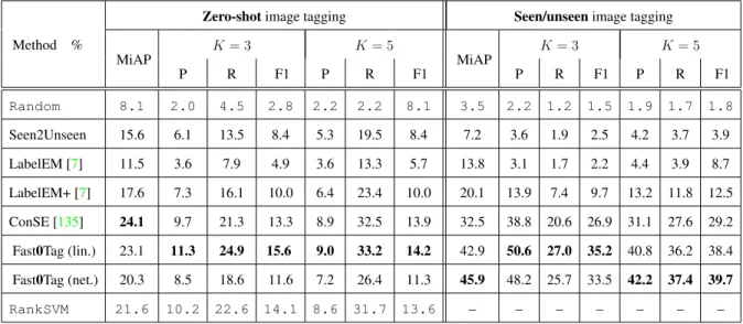
Table 3.5: Comparison results of the zero-shot and seen/unseen image tagging tasks with 58

unseen tags and 233 seen tags on IAPRTC-12.

Method %

Zero-shotimage tagging Seen/unseenimage tagging

MiAP K= 3 K= 5 MiAP K= 3 K= 5 P R F1 P R F1 P R F1 P R F1 Random 8.1 2.0 4.5 2.8 2.2 2.2 8.1 3.5 2.2 1.2 1.5 1.9 1.7 1.8 Seen2Unseen 15.6 6.1 13.5 8.4 5.3 19.5 8.4 7.2 3.6 1.9 2.5 4.2 3.7 3.9 LabelEM [7] 11.5 3.6 7.9 4.9 3.6 13.3 5.7 13.8 3.1 1.7 2.2 4.4 3.9 8.7 LabelEM+ [7] 17.6 7.3 16.1 10.0 6.4 23.4 10.0 20.1 13.9 7.4 9.7 13.2 11.8 12.5 ConSE [135] 24.1 9.7 21.3 13.3 8.9 32.5 13.9 32.5 38.8 20.6 26.9 31.1 27.6 29.2 Fast0Tag (lin.) 23.1 11.3 24.9 15.6 9.0 33.2 14.2 42.9 50.6 27.0 35.2 40.8 36.2 38.4 Fast0Tag (net.) 20.3 8.5 18.6 11.6 7.2 26.4 11.3 45.9 48.2 25.7 33.5 42.2 37.4 39.7

(49)

3.5.2 Results

Table 3.4 and 3.5 show the results of all the three image tagging scenarios (conventional,

zero-shot, and seen/unseen tagging). The proposed Fast0Tag still outperforms the other competitive

baselines in this new IAPRTC-12 dataset.

A notable phenomenon, which is yet less observable on NUS-WIDE probably due to its noisier seen tags, is that the gap between LabelEM+ and LabelEM is significant. It indicates that the traditional zero-shot classification methods are not suitable for either zero-shot or seen/unseen image tagging task. Whereas we can improve the performance by tweaking LabelEM and by carefully removing the terms in its formulation involving the comparison of identical images.