Abstract— A heuristic procedure based on novel recursive
formulation of sinusoid (RFS) and on regression with predictive least-squares (LS) enables to decompose both uniformly and nonuniformly sampled 1-d signals into a sparse set of sinusoids (SSS). An optimal SSS is found by Levenberg-Marquardt (LM) optimization of RFS parameters of near-optimal sinusoids combined with common criteria for the estimation of the number of sinusoids embedded in noise. The procedure estimates both the cardinality and the parameters of SSS. The proposed algorithm enables to identify the RFS parameters of a sinusoid from a data sequence containing only a fraction of its cycle. In extreme cases when the frequency of a sinusoid approaches zero the algorithm is able to detect a linear trend in data. Also, an irregular sampling pattern enables the algorithm to correctly reconstruct the under-sampled sinusoid. Parsimonious nature of the obtaining models opens the possibilities of using the proposed method in machine learning and in expert and intelligent systems needing analysis and simple representation of 1-d signals. The properties of the proposed algorithm are evaluated on examples of irregularly sampled artificial signals in noise and are compared with high accuracy frequency estimation algorithms based on linear prediction (LP) approach, particularly with respect to Cramer-Rao Bound (CRB).
Index Terms—Signal decomposition, Signal recovery, Sparse
set of sinusoids, Time series modeling, Predictive least squares
I. INTRODUCTION A. Problem statement
ET
{ }
wk Kk=1 denote a time series, where wk∈ℜ(
k=1,...,K)
is the kth observation obtained at the corresponding time point tk,{ }
K k k
t
=1. Suppose a time series representing a finite number of sine waves embedded in noise. Suppose also that a time series may have a nonzero mean value and/or a linear trend. The objective of this paper is spectral analysis and modeling of a time series outlined above and represented by:(
)
[
A t]
s k K t o w N k n n n k n k k sin , 1,..., 1 = + ∑ ⋅ ⋅ + + + = = ϕ ω κ , (1)This work has been supported by the Croatian Ministry of Science and Education through the project ‘‘Computational Intelligence Methods in Measurement Systems’’ No. 098-0982560-2565 within the Centre of Research Excellence for Data Science and Cooperative Systems.
I.Maric is with the Division of Electronics, Rudjer Boskovic Institute, Bijenicka 54, 10000 Zagreb, Croatia (e-mail: [email protected]).
where o and κ denote the corresponding y-intercept at t=0 and the slope of a linear trend line, An, ωn and φn are the
corresponding amplitude, radian frequency and phase of the
nth sine wave and sk represents the noise.
B. Related work
A non-uniform sampling is common to many long-time ground-based astronomical observations including spectra and time series (Lomb, 1976; Scargle, 1982). A number of papers dealing with the decomposition of a time series into a SSS are based on the least-squares spectral analysis and have been published very early. Methods based on the least-squares fit of sinusoids to data are introduced, also known as LS periodogram (LSP) analysis, formulated as LS fitting problem:
[ ] [ ]
(
)
∑ −∑ ⋅ ⋅ + = = − ∈ ∈≥ K k N n n n k n k A w A t n n n 1 2 1 , , 0 0 sin min maxϕ
ω
π π ϕω ω , (2)where ωmax denotes maximum expected angular frequency.
Frequency estimation methods can be divided into the two main classes: nonparametric and parametric. The nonparametric frequency estimation is based on the Fourier transform and its ability to resolve closely spaced sinusoids is limited by the length of sampled data. On the other hand the parametric approach enables to achieve a higher resolution since it assumes the generating model with known functional form, which satisfies the signal (So et al., 2005).
The earliest nonparametric frequency estimation methods are based on LSP analysis. Barning (1962) used least-squares fitting to calculate the amplitudes of sine waves from the corresponding frequencies selected from periodogram. Vaníček (1969) first proposed successive spectral analysis of equally spaced data and later he extended the analysis to nonumiformly sampled data (Vaníček, 1970). Lomb, (1976) analyzed statistical properties of irregularly spaced data based on periodogram analysis. He has shown that, due to the correlation between noise at different frequencies, noise has less effect on a spectrum than it could be expected. Scargle (1982) studied the use of periodogram with irregularly spaced data. He concluded that periodogram analysis and least-squares fitting of sine waves to data are exactly equivalent. Foster (1995) proposed a sequential method for removing false peaks from power spectra that can be viewed as Matching Pursuit (Mallat, & Zhang, 1993), a general procedure for computing adaptive signal representations
Retrieving sinusoids from nonuniformly
sampled data using recursive formulation
Ivan Maric
which decomposes any signal into a linear expansion of waveforms that are selected from a redundant dictionary of functions. Bourguignon, Carfantan, and Idier, (2007) estimated spectral components from irregularly sampled data. Sparse representation of noisy data is searched for in an arbitrarily large dictionary of complex-valued sinusoidal signals, which can be viewed as Basis Pursuit Denoising problem (Chen, Donoho, & Saunders, 2001). The nonparametric method for spectral analysis of nonuniform sequences of real-valued data named real-valued iterative adaptive approach (RIAA) is proposed by Stoica, Li, and He (2009). It can be interpreted as an iteratively weighted LSP. The method can be used for spectral analysis of general data sequences but is most suitable for zero-mean sequences with discrete spectra. Similar problems, dealing with sparse reconstruction, have been investigated recently in scope of compressed sensing, (Tang et al., 2012; Nichols, Oh, & Willett, 2014; Boufounos et al., 2012; Panahi & Viberg, 2014; Teke, Gurbuz, & Arikan, 2013), illustrating only signal reconstruction errors but not demonstrating that the proposed methods achieve a Cramer–Rao bound, above some SNR threshold, for all the real frequencies embedded in the signal.
Well-known parametric frequency estimation methods are maximum likelihood (ML) (Rife, & Boorstyn, 1976; Bresler & Macovski, 1986), and nonlinear least squares (NLS) (Stoica & Nehorai, 1988) and the methods based on linear prediction (LP) property of sinusoids like Yule–Walker equations (Chan, & Langford, 1982), total least squares, (Rahman, & Yu, 1987), iterative filtering (Li, & Kedem, 1994), MUSIC and ESPRIT (Porat, 2008), weighted least squares (So et al., 2005). Under additive white Gaussian noise the ML and NLS methods are equivalent and achieve Cramer–Rao lower bound (CRLB) asymptotically, but they are computationally demanding. The above mentioned methods, based on LP property, provide suboptimum estimation performance but they are computationally efficient. The parametric methods based on linear prediction (Chan, Lavoie, & Plant, 1981; So, et al., 2005; Dash, & Hasan, 2011; Yang, Xi, & Guo, 2007) enable to retrieve the sinusoids from a uniformly sampled sinusoidal signal in noise when the number of sinusoids in the signal is known a priori. So et al. (2005) developed two high accuracy frequency estimators for multiple real sinusoids in white noise based on the LP approach. First, they developed a constrained least squares frequency estimator named reformulated Pisarenko harmonic decomposer (RPHD) and then they improved it through the technique of weighted least squares (WLS) with a generalized unit-norm (WLSun) and monic (WLSm) constraint. The method assumes uniformly sampled data and the number of sinusoids to be known a priori.
The heuristic procedure elaborated in this paper is also based on the LP property of a sinusoid and is intended for recovery of frequency-sparse signals in noise. It can be used in signal processing, machine learning and expert and intelligent systems to facilitate solving the classification, diagnosis, monitoring or process control tasks needing analysis and parsimonious representation of signals, including the signals in technical systems, bio-signals, astronomical observations,
etc. The proposed algorithm enables to retrieve the sinusoids from either uniformly or nonuniformly sampled data. In order to adapt it to nonuniform sampling we first reformulate the LP property of a sinusoid and we named it a recursive formulation of a sinusoid (RFS). Then we formulate a sinusoidal model based on RFS and the corresponding procedures for the estimation of RFS parameters based on the minimization of LS error. By combining the RFS approach with the well-known methods for the estimation of the number of sinusoids in noise the proposed procedure enables to retrieve the sinusoids iteratively, one at a time, and to determine the order of the generating model. The proposed method assumes neither a zero mean sequence nor the number of sinusoids in a signal to be known a priori. The accuracy of the frequency estimation procedure proposed in this paper is compared with very high accuracy of frequency estimation obtained by LP approach reported by So et al. (2005). For a frequency-sparse signal the computational complexity of both methods is comparable, O(K3).
C. Methods for detection of the number of sinusoids
Most parametric methods for detection of sinusoids corrupted with noise minimize the sum of a data fit (likelihood) term and the complexity penalty term where the penalty term is usually derived via Akaike information criterion (AIC) (Akaike, 1974), Bayesian information criteria (BIC) (Schwarz, 1978) or minimum description length (MDL) (Rissanen, 1978). A review of information criterion rules for model-order selection with the summary of necessary steps used to adapt a rule to a specific problem is given in Stoica and Selen (2004). In this paper the attention is restricted to efficient detection criteria (EDC) type estimators (Djurić, 1996, 1998; Nadler & Kontorovich, 2011). EDC type estimators determine the number of sinusoids by minimizing:
(
M)
K M L , MC M= − + =β
w ) ) ln min arg ... 2 , 1 , 0 , (3)where w is the observed time series of length K, M β
)
are parameter estimates of a model of order M, L
(
β)M,w)
is the corresponding likelihood term and CK is the model-complexitypenalty term that captures the dependency of the penalty on the number of samples K. For the unknown noise level the log-likelihood term in (3) can be approximated by:
(
)
[
( )
]
0.5 1 2 , ln 2 ln ∑ − − = = K k k Mk M M w P K , Lβ) w β) , (4) where PMk( )
βM ), denotes the approximation of wk at time point
tk made by a model of order M. By substituting (4) for
log-likelihood in (3) we obtain:
( )
[
]
K K k k Mk M M w P MC K M + ∑ − = = = 5 . 0 1 2 , ,... 2 , 1 , 0 2 ln min arg β) ) . (5)model with maximum a posteriori probability (MAP) criterion for sinusoids with unknown frequencies amplitudes and phases Djurić (1996) derived the following penalty term
(
M)
KCK = 5 2ln (6)
and he concluded that the parameters that can be determined more precisely should receive stronger penalty. Nadler and Kontorovich (2011) proposed the estimator inspired by ideas from extreme value theory (EVT) and the maxima of stochastic fields with the following penalty term
− + =
π
α
2 3 ln 2 1 ln ln 2 1 lnK K CK , (7)where α<<1 denotes a confidence level chosen by the user, typically α≤0.005. They recommend the generalized likelihood ratio test (GLRT)
(
)
(
)
K M M C , L , L > − w w 1 lnβ
β
) ) (8)to determine the number of sinusoids (M).
Next section elaborates the RFS and the RFS-based regression procedures and the corresponding RFS-based algorithm (RFSA) used to retrieve the sinusoids from nonuniformly sampled data. In Section III the frequency estimation accuracy of the proposed procedure is compared with high accuracy LP approach (So et al., 2005). Also the results of spectral analysis of a couple of nonuniformly sampled 1-d signals are given to illustrate the properties of the proposed method.
II. TIME SERIES ANALYSIS BY RFS
This section presents a novel RFS based procedure for retrieving the sinusoids from unevenly spaced data. The proposed procedure is able to precisely estimate the total number and the parameters of SSS from uniformly and nonuniformly sampled sinusoidal signal in noise. It can discover a cyclical pattern with linear trend in data (e.g. excitation signals in AC voltammetry, atmospheric Carbon Dioxide data) or to retrieve an undersampled sinusoid or a low frequency sinusoid in cases when only a fraction of its cycle is covered by a time series. The procedure is based on minimization of accumulated prediction error using l2-norm.
The frequencies from a predefined set of frequencies are optimized individually by LM (Levenberg, 1944; Marquardt, 1963) in order to obtain the parameters of a sinusoid which best minimizes the predictive LS error. Next, LM optimization is used to fine tune the RFS parameters of all most dominant sine waves found until then, resulting with a decomposition of a time series into an optimal set of sinusoidal components. In order to determine the cardinality of a SSS, the procedure combines the criteria for the detection of the number of
sinusoids embedded in noise (Nadler & Kontorovich, 2011; Djurić, 1996; Djurić, 1998) (see Section I–C).
The idea of RFS in nonuniform and uniform sampling case and its adaptation for straight line approximation is given below, followed by a reformulation of the LS fitting problem (2) in terms of sine wave representation by a RFS. Next, the procedure for calculating pairs of initial samples of the sinusoids is presented, then the elaboration of the LM optimization of RFS parameters is given and finally the explanation of RFS model order estimation procedure, which rounds up the methodology. The section concludes with the description of the RFSA algorithm.
A. Recursive Formulation of a Sinusoid and a Straight Line 1) Nonuniform sampling case
A sinusoid ym = Amsin
(
ωmt+ϕm)
can be predicted by using a simple RFS (see Appendix A), which relates any sample of a sinusoid with its two referent samples, e.g. two initial samples: 1 , , 2 , , ,k mk m mk m m a y b y y = + (9)where m denotes a sine wave with the corresponding radial frequency (ωm), amplitude (Am) and phase (φm), ym,k denotes
the predicted magnitude of the sine wave at time point tk, ym,1
and ym,2 represent two initial samples obtained at the
corresponding time points t1 and t2, am,k and bm,k are time and
frequency dependent coefficients defined as
(
)
(
2,1)
1 , , sin sin τ ω τ ω m k m k m a = (10) and(
)
(
2,1)
2 , , sin sin τ ω τ ω m k m k m b =− (11) with i j i j, =t −tτ representing the difference in seconds between the time points of jth and ith sample from the sequence of samples and ωm denoting angular frequency of the sine wave
in rad/s. Note that the radian frequency and the two initial samples (ωm, ym,1, ym,2) are the parameters of RFS (9), which
completely specify the corresponding sinusoid.
If ωm →0, (10) and (11) can be replaced by
1 , 2 1 , ,k
τ
kτ
m a ≈ and bm,k ≈−τ
k,2τ
2,1, respectively.Substituting τk,2=τk,1–τ2,1 in bm,k and then am,k and bm,k in (10)
the following approximate equation is obtained:
1 , 1 , 1 , 2 1 , 2 , 0 , k m m m k m y y y y m + − ≈ → τ τ ω , (12)
which can be recognized as a recursive formulation of an arbitrary straight line. Hence, for the given angular frequency
[
0,ωmax]
ωm∈ and the two initial samples ym,1 and ym,2 with the
corresponding time points t1 and t2, any sample ym,k of a sine
wave, including a straight line as a special case when ω=0, can be accurately predicted at the time point tk by using (9)–(12).
2) Uniform sampling case
In case of uniform sampling the coefficients (10) and (11)
become
[
(
)
]
(
T)
T k a m m k m ω ω sin 1 sin , − = and[
(
)
]
( )
T T k bmk ω ω sin 2 sin , − − = ,where T denotes a sampling period and the coefficients are now calculated recursively by adapting Chebyshev multiple angle formula, i.e.
1 , 1 , ,k = m mk− + mk− m x a b a (13) 1 , ,k =− mk− m a b (14) where am,1=0, bm,1=1, and
(
T)
xm=2cosω
m . (15)Note that in uniform sampling case the parameter xmϵ[-2,2] is
equivalent to frequency parameter ωmand the calculation of
the coefficients (13) and (14) is reduced to FP multiplications and additions only. After the parameter xm is estimated, it can
be easily converted into the frequency
(
x
m)
T
mcos
/
2
/
1 −=
ω
. (16)Note that Eqs. (13)– (16) are valid for both, a sinusoid and an arbitrary straight line (ωm=0 ⇔ xm=2).
B. Reformulation of LS Fitting Problem
After substituting the RFS (9) for each sinusoidal component, including a trend line (12), the time series (1) can be represented by the following relation:
(
a y b y)
s k K w M k m mk m mk m k , 1,..., 1 , ,2 , ,1 = + ∑ + = = , (17)where am,k and bm,k denote the coefficients (10) and (11) of the
mth RFS (9) and N in (1) is replaced by M=N+1 in (17) because additional RFS in (17) is used to represent a linear trend in data (1). Recall that recursive formulation of a straight line (12) is a special case of RFS (9) when the frequency of a sinusoid approaches zero. Note that two initial samples ym,1
and ym,2 in each RFS m=1,…,M in (17) and the corresponding
angular frequency ωm, which affects the coefficients am,k (10)
and bm,k (11) are all considered independent variables. Hence,
the sinusoidal signal can be restored from noisy data sequence (17) if the initial samples and the frequencies of the corresponding sinusoids can be estimated. The LS fitting problem (2) is re-formulated in the following way:
[ ] [ ]
(
)
∑ −∑ + = = = − ∈ ∈ +∞ ∞ − ∈ +∞ ∞ − ∈ K k M m mk m mk m k x or y y M w a y b y E m m m m 1 2 1 , ,2 , ,1 2 , 2 , , , max min 2 , 1 , min ω ω ω , (18)where ωmin and ωmax denote the corresponding lower and
upper bound for possible angular frequencies
[
ωmin,ωmax]
ωm∈ and M is the number of detected sinusoids. The LS fitting of RFS to data (18) is different from (2) since it employs prediction rather than approximation to estimate RFS parameters β,
{ }
{
m m m}
mM M m m =1=ω
,y ,1,y ,2 =1β
, or{ }
{
}
M m m m m M m m =1= x ,y,1,y ,2 =1β
in the uniform sampling case, byminimizing the error function based on predictive least squares (Rissanen, 1986). If it would be possible to estimate the RFS parameters, by solving the LS fitting problem (18), then it should also be possible to reconstruct the time series (17) or (1) as well as to calculate the amplitudes and phases of all sine waves (see Appendix C).
To solve the LS fitting problem (18) the following procedures are necessary:
1. Calculation of initial samples of sine waves that best minimize (18) for the given angular frequencies (see Section II–D).
2. Optimization of parameters (frequencies and initial samples) of multiple RFS by LM algorithm (see Section II–E).
This new formulation, when applied to nonuniformly sampled data representing multiple superimposed oscillations (MSO), enables to recover the sinusoid even if sampled data represent only a fraction of its cycle as well as to recover the under-sampled sinusoid whose frequency might be higher than the Nyquist frequency defined by the Nyquist–Shannon sampling theorem (Shannon, 1998). In case of nonuniform sampling the Nyquist frequency can be pushed very high (Eyer & Bartholdy, 1999; Koen, 2006). For the given angular frequency ωx, the proposed procedure maps all nonuniformly
spaced angles into the same normalized sine wave period [0, 2π], using the relation mod2π(ωxtk+φx), thus artificially
shortening the average sampling period. The design of optimal sampling pattern is beyond the scope of this paper.
C. RFS Model Estimation
Let
{ }
K k kw =1 be a nonuniform time series with the corresponding time points
{ }
Kk k
t =1 represented by (1) or equivalently by (17). A solution to LS fitting problem (18) is the following RFS model of a time series:
( )
y(
a y b y)
k K P M m mk m mk m M m mk k M , 1,..., 1 , ,2 , ,1 1 , , = ∑ = ∑ + = = = β (19)where PM,k(β) denotes the predicted value of kth sample of a
time series represented by a superposition of M RFS. The time and frequency dependent coefficients am,k and bm,k are defined
need to estimate the RFS parameters β. The corresponding algorithm (see Section II–G) iteratively estimates the most dominant sinusoids in the signal. It uses predefined frequencies to find the suboptimal RFS parameters close to real RFS parameters (Section II–D), then it optimizes RFS parameters (Section II–E) trying to solve the LS fitting problem (18). The procedure starts with estimation and optimization of RFS parameters of the first most dominant sinusoid, than continues with the estimation and optimization of the RFS parameters of the two most dominant sinusoids etc. The procedure combines EDC estimators to select the model order.
D. Calculation of Initial Samples of Sine Waves
This section details the calculation procedure, which enables direct solution to (18) for M predefined frequencies. Given the frequencies,
{ }
Mm m =1 ω , or
{ }
M m m x =1 in the uniform sampling case, the LS prediction error (18) has to be minimized with respect to initial samples of sinusoids α,{ }
{
}
M m m m M m m =1= y ,1,y ,2 =1α
, where the coefficients am,k and bm,kin (18) are calculated by (10) and (11) using the preselected frequencies
{ }
Mm m =1
ω , or in case of uniform sampling by (13) and (14) using the preselected parameters (15),
{ }
Mm m
x =1. Note that α is a subset of β, α⊆β. After setting the partial derivatives of (18) with respect to initial samples equal to zero a set of 2M simultaneous linear equations in matrix form is obtained:
( )
JTJα=JTw, (20)where w is a time series vector, α is a parameter vector to calculate and J is a Jacobian matrix of time series prediction model PM,k(ββββ) (16) with respect to α, α⊆β, (see Appendix B).
Eq. (20) can be solved directly forα.
E. Optimization of RFS parameters by LM algorithm
The parameter vector β of the RFS model (19), obtained in Section II–C, can be optimized by LM algorithm (Levenberg, 1944; Marquardt, 1963) in order to further minimize the LS error (18). LS fitting problem (18), adapted for LM optimization takes the form of a nonlinear error function:
(
)
[
(
)
]
∑ ∑ ∂ ∂ + ∂ ∂ + ∂ ∂ + − ≈ ≈ ∑ − + = + = = = K k M m m m k m m m k m m m k m k m k K k k Mk LM y y y y y y y y w P w E 1 2 1 ,2 ,2 , 1 , 1 , , , , 1 2 , δ δ δω ω δ β δ β , (21)where δ denotes the parameter increment vector to calculate,
{ }
{
}
M m m m m M m m =1=δω
,δ
y ,1,δ
y ,2 =1δ
or{ }
{
}
M m m m m M m m =1=δ
x ,δ
y ,1,δ
y ,2 =1δ
, and β is the parameter vector tooptimize. Note that in case of uniform sampling the parameter
xm has to be substituted for ωm in (21) and in ββ and ββ δ. After
setting the partial derivatives of (21) with respect to increments equal to zero and after introducing an adjustable nonnegative damping factor γ and the diagonal matrix of JTJ, where J is a Jacobian matrix of a time series model PM,k(β)
(19) with respect to parameters β, a well-known LM equation in matrix notation is obtained:
( )
[
JTJ+ ⋅ JTJ]
δ=JT[
w−P( )
β]
diag
γ , (22)
summarizing a set of 3M linear equations with 3M unknowns (δ). A more detailed description of (22) is given in Appendix D. Over a preset number of steps L the LM algorithm successively modifies the parameter vector (βl+1=βl+δl) by the
lth instance of the increment vector (δ), obtained from (22). In nonuniform sampling case the partial derivatives of ym,k with
respect to ωm, ym,1 and ym,2 in (21) are derived from (9) after
substituting (10) and (11) for am,k and bm,k, respectively:
(
)
(
2,1)
2 , 1 , , sin sin τ ω τ ω m k m m k m y y − = ∂ ∂ , (23)(
)
(
2,1)
1 , 2 , , sin sin τ ω τ ω m k m m k m y y = ∂ ∂ . (24)(
) (
)
(
)
[
]
(
) (
)
(
)
[
]
(
) (
)
(
)
[
]
(
) (
)
(
)
[
]
2 ,1 1 , 2 1 , 2 2 , 1 , 2 1 , 2 1 , 2 1 , 2 2 , 2 , 2 , 2 1 , 2 1 , 2 1 , 1 , 2 2 , 2 1 , 2 1 , 2 1 , 1 , , sin cos sin sin sin cos sin cos sin sin sin cos m m m k m m m m k m k m m m k m m m m k m k m k m y y y y y τ ω τ ω τ ω τ τ ω τ ω τ ω τ τ ω τ ω τ ω τ τ ω τ ω τ ω τ ω + − − = ∂ ∂ , (25)The partial derivatives (23) – (25) are derived by assuming the mutual independence of the RFS parameters:
0 1 , 2 , 2 , 1 , 2 , 1 , = ∂ ∂ = ∂ ∂ = ∂ ∂ = ∂ ∂ m m m m m m m m y y y y y y ω ω and ,2 1 2 , 1 , 1 , = ∂ ∂ = ∂ ∂ m m m m y y y y . (26)
In uniform sampling case the partial derivatives of ym,k with
respect to xm, ym,1 and ym,2 in (21) are derived from (9) after
substituting (13) and (14) for am,k and bm,k, respectively:
1 , 1 , , − − = ∂ ∂ k m m k m a y y , (27) 1 , 1 , 2 , , − − + = ∂ ∂ k m k m m m k m b a x y y . (28) 1 , , 2 , , , m m k m m m k m m k m y x b y x a x y ∂ ∂ + ∂ ∂ = ∂ ∂ , (29)
where m k m m k m m k m m k m x b x a x a x a ∂ ∂ + ∂ ∂ + = ∂ ∂ − − − 1 , 1 , 1 , , , (30) m k m m k m x a x b ∂ ∂ − = ∂ ∂ , ,−1 , (31) and where ,1 ,1=0 ∂ ∂ = ∂ ∂ m m m m x b x a .
Note that the components of partial derivatives am,k, bm,k,
∂am,k/∂xm and ∂bm,k/∂xm can be calculated completely
recursively by using FP multiplications and additions only.
F. Error minimization and RFS model order selection
The RFS approach can be efficiently combined with well-known criteria for detection of the number of sinusoids embedded in noise. The number of sinusoids is estimated by following the procedure outlined in Stoica, Li, and He (2009). Let
{
}
M m m m m M = ,y ,1,y ,2 =1 ( ( ( (ω
β (32)denote the RFS parameters of the corresponding M sinusoids used to approximate the time series by the RFS model (19). The corresponding errors (18), due to the approximation of a time series by a certain number M=1,2,…,Mmax of
superimposed sinusoids, are arranged in a decreasing order of their values: max ... 2 1 E EM E ≥ ≥ ≥ . (33)
Note that the RFS parameters (32) obtained in the preceding steps are optimized in each succeeding step by LM ((21) and (22)) with the aim to minimize the error (18).
Under the idealizing assumptions that a time series consists of a finite number of sinusoidal components and of normal white noise, and that (18) represents maximum likelihood (ML) estimates of frequencies and initial samples of Mmax such
sinusoidal components, the EDC(M) is used to select M in (5), where EDC(M) is obtained after substituting (19) for PM,k
( )
β)M in (5). If a time series consists of white noise only, {wk}={sk},then according to (5) M=0 is selected with the corresponding
EDC(0):
( )
[ ]
0.5 1 2 ln 2 0 ∑ = = K k k w K EDC (34)Note that in case of uniform sampling the parameter xm
needs to be optimized, instead of ωm, to minimize the error.
G. RFSA
This section describes the algorithm (RFSA) for decomposition of a time series into an optimal SSS. The basic steps of the algorithm are outlined in Table I. The procedure is iterative with the corresponding initial guess: M=0
) ,
{ }
= 0 β (and E0=EDC(0) defined by (34). In each succeeding
cycle (M=1,2,…,Mmax) a set of predefined trial frequencies
{ωj}, j=1,…,J is used to estimate the current (Mth) most
dominant frequency in a time series. Each trial frequency is separately appended to the set of most dominant frequencies obtained in the preceding cycle and each time (20) is solved to estimate the initial samples of M sine waves that best minimize (18). The best obtained set of RFS parameters (including the frequencies) is then optimized by LM (22) in order to further decrease the prediction error (21). In each cycle the RFS parameters βM
(
that best minimize (21) are saved along with the corresponding EDC(M) used in (5). When the condition M≥Mmax has been satisfied, the model
order M
)
(5) and the corresponding RFS parameters M)
(
β are determined. The GLRT stopping criterion (8) slightly increases the probability of underestimation of the number of sinusoids in high noise and is therefore not embedded in RFSA. Note that the product of angular frequency and sampling interval ωmτ2,1 may cause an overflow error when
calculating (10), (11), (23), (24) and (25). To prevent the possible errors the following constraint is implemented in software: if sin│ωmτ2,1│<δ, where │δ│=10–12, then set
sin(ωmτ2,1) equal to –δ or +δ depending on the negative or
positive sign of sin(ωmτ2,1), respectively. The RFSA algorithm
outlined in Table 1 is the same for uniform sampling case except that parameter x (15) has to be optimized instead of frequency ω using the corresponding parameter range limits
xmin=–2 and xmax=2 instead of ωmin and ωmax, respectively. TABLEI
DECOMPOSITION OF TIME SERIES INTO THE OPTIMAL SSS BY RFSA Input
time series {wk}, lowest (ωmin) and highest (ωmax) expected radian
frequency, total number of trial frequencies (J), maximum number of sinusoids (Mmax), maximum number of LM optimization steps (L)
Initialization 0 = M ) , β0=
{ }
( , =∑ 2 0 wk eIteration – main loop For M=1 to Mmax step 1
eM=eM-1
For j=1 to J step 1
ωj=ωmin+(j–1)·(ωmax–ωmin)/(J–1)
βM =βM−1+
{
ωj,0,0}
( Solve EM(ββββM) for αM⊆ββββM (20) If eM>EM(ββββM) Then eM=EM(ββββM) and βM =βM ( Next j Optimize βM ( by LM (22) in up to L steps to minimize ELM, (21)Calculate and save the corresponding EDC(M), (5). Next M
Results
Return the model order M )
(5) and the RFS parameters M)
(
To retrieve each new sinusoid the algorithm has to solve (20) and (22) repeatedly. For M<<K, the complexity of (20) and (22), when estimating M sinusoids, is O
(
MK2)
. Since (20) has to be solved J times and (22) L times to retrieve each new most dominant sinusoid, the overall complexity of the algorithm is O(
(J+L)MmaxK2)
, where J, L and Mmax are thepreset numbers of trial (grid) frequencies, LM optimization steps and maximum expected sinusoidal components, respectively. The complexity can be reduced significantly if (20) is solved for all J trial frequencies in parallel i.e.
(
2)
maxK
M L
O ⋅ .
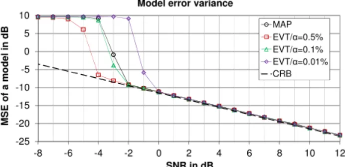
III. RESULTS OF TIME SERIES ANALYSIS BY RFSA This section describes the results of analysis and modeling of an irregularly sampled MSO. Examples of artificial MSO embedded in noise are given. The accuracy of frequency estimation of RFSA will be compared with high accuracy frequency estimation algorithms based on LP approach (So et al., 2005) in Section III–A, and in the succeeding sections it will be demonstrated how RFSA can efficiently recover under-sampled sinusoid and a sinusoid represented by a fraction of its cycle (Section III–B), two closely spaced sinusoids with linear trend (Section III–C), three closely spaced sinusoids (Section III–D), and 10 sinusoids (Section III–E). Nonuniformly sampled signals with additive noise are considered in all examples. The results are obtained by minimizing EDC (5) with respect to M and by applying the two model-complexity penalizations: MAP (6) and EVT (7). Some general remarks are given in Section III–F.
The CRB for irregular sampling is hard to calculate. It was shown experimentally (Larsson & Larsson, 2002) that CRB is practically the same, but not identical, for different sampling schemes having the same average sampling interval. Hence, the CRB for uniform sampling can be used to approximate the CRB for nonuniform sampling if the average sampling interval of the nonuniform sampling pattern is equal to sampling interval in uniform sampling. To approximate the bound on the frequency for the case of nonuniform sampling the CRB (Porat, 2008, page 265), can be rewritten in the following way: + ≈ ) sin( ) sin( ) 2 cos( 3 1 24 ) ( 3 2 2 2 m m m m m K K A K CRB
ω
ω
ϕ
τ
σ
ω
, (35)where
τ
denotes the mean sampling interval in seconds and σ2 is the noise variance.The signal-to-noise ratio (SNR) for mth sinusoid is defined as 2 /2σ2 m A or in dB units: = 2 2 10 2 log 10
σ
m m A SNR dB, (36)where Am is the amplitude of the mth sinusoid. The additive
noise is white with zero mean. In all figures the SNR is given with respect to a sinusoid with amplitude A=1, i.e.
SNR=1/(2σ2) , except in figures in Section III–A, where A=20.5 and SNR=1/σ2. In all examples the maximum number of LM optimization steps is 30 and the LM damping factor is 1.5. The RFSA is coded in Visual C and executed on Intel®Xeon® CPU E5420 @ 2.50 GHz. To illustrate the computational complexity of the procedure the maximum computation time needed to decompose a single time series is given in each example.
A. Comparing RFSA with high accuracy frequency estimation algorithm
The accuracy of frequency estimation of the RFSA is compared with LP-based high accuracy frequency estimation algorithm proposed by So et al., (2005). The algorithms have approximately equal computational complexity. The results obtained by RFSA are compared with the results published by
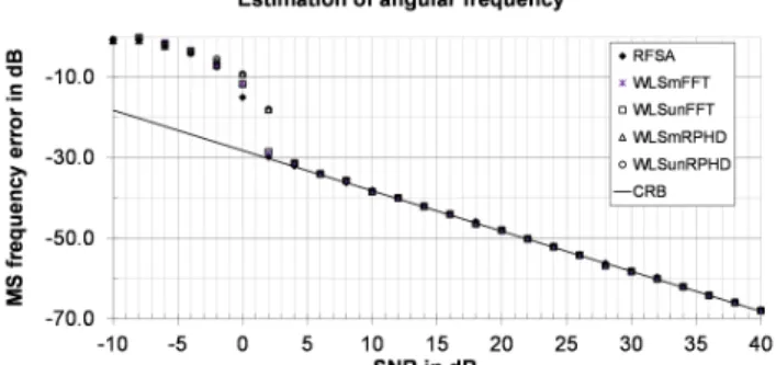
So et al. (2005). Fig 1 shows a mean squared error (MSE) of frequency of a single sinusoid y=20.5sin(0.3π) in white Gaussian noise obtained from uniformly sampled data (T=1s) with K=20 samples. SNR values in the range [–10, 40] dB are considered in this experiment. For each SNR value 1000 Monte Carlo (MC) trials are performed. The frequency interval fϵ[0,0.5] Hz (fϵ[0,π] rad/s) is used in RFSA with 0.5/19 Hz (π/19 rad/s) as a step of a frequency grid (J=20 frequencies) and the maximum preset order of a model is
Fig. 1. MSE of the frequency versus SNR obtained by RFSA from irregular data sequences (K=20) using EVT model order estimator (7) with α=0.1% and 20 trial frequencies.
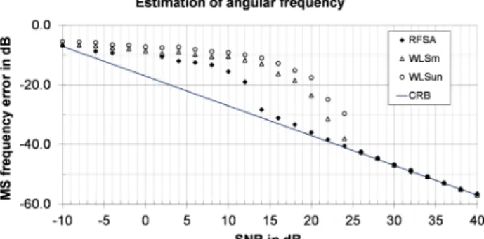
Fig. 2. MSE of the frequency versus SNR obtained by RFSA from irregular data sequences (K=1000) using EVT model order estimator (7) with α=0.5% and 20 trial frequencies.
Mmax=4. EVT penalization (7) is used with confidence level α
=0.1%. From Fig 1 it can be seen that MSE obtained by RFSA is almost identical to MSE obtained by WLS with monic and unit norm constraints when initiated by FFT (WLSmFFT and WLSunFFT) or RPHD (WLSmRPHD and WLSunRPHD). All methods have SNR threshold at about 2dB and attained the CRB for sufficiently high SNR conditions. Note that, unlike the methods published by So et al. (2005), RFSA does not need the number of sinusoids in the signal to be known a priori and it selected correct model order (M=1) in the entire range of SNR. Maximum execution time of RFSA for a single trial was 0.385 s. The same test was repeated for K=1000. The frequency interval fϵ[0,0.5] Hz (fϵ[0,π] rad/s) is used in RFSA with 0.5/999 Hz (π/999 rad/s) as a step of a frequency grid (J=1000 frequencies) and the maximum preset order of a model is Mmax=4. The results shown in Fig. 2 are obtained
from uniformly sampled data (T=1s). The SNR range [–20, 40] dB is considered. EVT penalization (7) is used with confidence level α =0.5%. The RFSA correctly selects the model order (M=1) in the entire range of SNR and attained the CRB at threshold SNR≈–12dB. Maximum execution time of RFSA for a single trial was 12.8 s. The MSE reported by So et al. (2005) is given in the shorter SNR range [–10, 40] dB and attained the CRB over the entire range for the WLS initiated by FFT. The results obtained by WLS method when initiated by RPHD are considerably worse.
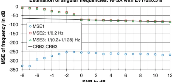
Finally the estimation of the frequencies in the three tone case y=20.5sin(0.3π)+2–0.5sin(0.34π)+2–0.5sin(0.7π) is considered. The SNR values are varied in the range [–10, 40] dB. For each SNR value 1000 MC trials are performed. The frequency interval fϵ[0,0.5] Hz (fϵ[0,π] rad/s) is used in RFSA with 0.5/19 Hz (π/19 rad/s) as a step of a frequency grid (J=20 frequencies). In this particular case the RFSA tends to
overestimate the model order. To prevent overestimation we set the maximum order of a model equal to the actual number of sinusoids in a model (Mmax=3) what can be considered
equivalent to the condition when the number of sinusoids is known a priori. The MSE for the lowest frequency (0.3 rad/s), obtained from uniformly sampled data (T=1s) with K=20 samples, is shown in Fig 3. EVT penalization (7) is used with confidence level α =0.5%. From Fig 3 it can be seen that RFSA attains CRB at significantly lower SNR threshold than
the WLS methods. Almost identical results have been obtained for other two frequencies (0.34π and 0.7π). Maximum execution time of a single trial was 0.098 s. From Figs 1–3 it can be concluded that under the same conditions RFSA achieved frequency estimation accuracy at least equal to or better than the accuracy reported by So et al. (2005).
B. Two sinusoids: one represented by a fraction of its cycle the other one under-sampled
To illustrate the other possibilities of time series analysis by RFSA let us consider an irregularly sampled 1-d signal consisting of M=2 superimposed sinusoidal components where the sampled data (64 samples) represent a fraction of the cycle of the first sinusoid whereas the second sinusoid can be considered under-sampled as the time interval between any two adjacent samples is always longer than the full period of the sinusoid. The frequencies of the sinusoids are f1=0.011 Hz
and f2=2.2 Hz and their amplitudes are: A1=1 and A2=0.5. The
sampling times are calculated by tk+1=tk+τk+1,k; k=1,2,…,64,
where t1=1s and the sampling intervals are uniformly and
independently distributed over the interval τk+1,k ϵ[0.5, 1.5] s
with mean
τ
k+1,k≈1s. Note that minimum sampling intervalequals 0.5 s and the Nyquist frequency ≤1 Hz is expected. The phases are φ1=0 rad and φ2=π/3 rad and the additive noise
is white and normally distributed with zero mean. SNR values in the range [–5, 22] dB are considered in the experiment. The frequency interval fϵ[0,4] Hz (fϵ[0,8π] rad/s) is used in RFSA with 4/511 Hz (2π/511 rad/s) as a step of the frequency grid (512 frequencies). A refined frequency grid enables precise estimation of very low frequencies. Maximum preset order of a model is Mmax=5. For each SNR value 500 Monte Carlo
(MC) trials are performed. Note that the corresponding sampling pattern and additive noise are randomized in each new MC trial. The RFSA sequentially estimates the RFS parameters of most dominant sinusoids and uses MAP and EVT estimators with the corresponding penalization terms (6) and (7) to estimate the number of sinusoids in a model. Given the sampling times and the estimated RFS parameters, the corresponding amplitudes and phases of the sinusoids can be calculated by following the procedure outlined in Appendix C. Each sinusoid can be easily reconstructed by (9) using its RFS parameters or by calculating its frequency, amplitude and phase (Appendix C).
Fig 4 shows an estimated probability of correct model order selection (M=2) by RFSA for MAP and EVT estimators with respect to SNR. Fig 5 shows a MSE of two angular frequencies estimated by RFSA from 500 Monte Carlo trials by using MAP model selection criteria (6). Almost identical chart is obtained by using EVT (7) with α=0.5%. From Fig 5 it can be concluded that the threshold for the frequency 0.011 Hz (MSE1) is at SNR≈2 dB and for the frequency 2.2 Hz (MSE2) at SNR≈9 dB. Above these thresholds the MSE approaches to CRB. Note that SNR values in Fig 5 correspond to the 1st sinusoid (A1=1) and are actually lower for about 6 dB for the
2nd sinusoid (A2=0.5). The RFSA estimates both the model
order and the frequencies. From Fig 4 it can be seen that correct model selection begins above SNR≈8 dB for model
Fig. 3. MSE of the frequency versus SNR obtained by RFSA from irregular data sequences (K=20) using EVT model order estimator (7) with α=0.5% and 20 trial frequencies.
selection criteria MAP (6) and EVT (7) with confidence level α =0.5%. Maximum execution time of a single trial was 1.46 s.
Fig 6 illustrates an instance of irregular sampling pattern
with the corresponding data embedded in noise (SNR= 7 dB). Time frame begins at 1 s and ends with 65.10 s. The RFS parameters of the correct model, obtained by the RFSA from data sequence (Fig 6) using MAP estimator (6), are given in Table II. Table III shows true amplitudes, frequencies and phases (subscript T), and the corresponding estimates (subscript E), obtained from RFS parameters (Table II) in accordance with Appendix C. Evidently, the RFSA is able to
precisely estimate the low frequency (0.011 Hz) represented
by a fraction of its cycle and the under-sampled frequency (2.2 Hz), which is higher than the Nyquist frequency (1 Hz) based on the minimum sampling interval (0.5 s).
C. Two closely spaced sinusoids with linear trend
A data sequence consists of a trend line κtk+o with fixed y–
intercept o=0.5 and a slope κ=0.006 s–1 and 2 sinusoidal components Amsin(2πfmt+φm), m=1,2 with the corresponding
amplitudes A1=A2=1, phases φ1=0 rad and φ2=π/4 rad and
frequencies f1=0.2 Hz and f2=0.2+1/K Hz, where K is the
number of samples in the sequence. The additive noise is white and normally distributed with zero mean. The data
Fig. 4. Estimated probability of correct model order selection (M=2) obtained by MC simulations (500 MC trials per SNR value) of irregular data sequence (K=64) representing two sinusoids: one with incomplete cycle and the other one under-sampled. 0.0 0.2 0.4 0.6 0.8 1.0 -5 0 5 10 15 20 E s ti m a te d p ro b a b il it y o f c o rr e c t m o d e l s e le c ti o n SNR in dB Model order selection
MAP EVT/α=0.5% EVT/α=0.1% EVT/α=0.01%
Fig. 5. MSE of the frequencies of sinusoids versus SNR obtained by RFSA from irregular data sequences (K=64) using MAP model order estimator (6). Circles and squares represent the MSEs and solid and dashed lines represent the CRBs for the corresponding frequencies.
-75 -50 -25 0 25 -5 0 5 10 15 20 M S E o f fr e q u e n c y i n d B SNR in dB
Estimation of angular frequencies: RFSA with MAP MSE1: 1/0.011 Hz MSE2: 0.5/2.2 Hz CRB1 CRB2
Fig. 6. An instance of irregular sampling pattern (K=64) illustrated by vertical lines with data sequence (dots) representing two sinusoids embedded in noise, SNR=7 dB. -2 -1 0 1 2 0 10 20 30 40 50 60 A m p li tu d e Time in seconds
Instance of sampling pattern with data sequence
Sampled data SNR = 7 dB
TABLEII
ESTIMATED RFSPARAMETERS OF THE MODEL
Component 1 2
ω [rad] 6.8901E–02 1.3822E+01
y1 4.7207E–02 3.1457E–01
y2 9.5103E–02 3.0437E–01
TABLEIII
TRUE AND ESTIMATED PARAMETERS OF SINUSOIDS
Component 1 2 AT 1 0.5 fT [Hz] 0.011 2.2 φT[rad] 0 π/3 AE 9.0025E–01 5.1729E–01 fE [Hz] 1.0966E–02 2.1998E+00
φE[rad] –1.6439E–02 1.2324E+00
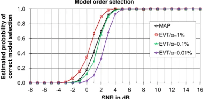
Fig. 7. Estimated probability of correct model order selection (M=3) obtained by MC simulations (500 MC trials per SNR value) of irregular data sequence (K=64) consisting of two closely spaced sinusoids with linear trend.
0.0 0.2 0.4 0.6 0.8 1.0 -5 0 5 10 15 20 E s ti m a te d p ro b a b il it y o f c o rr e c t m o d e l s e le c ti o n SNR in dB Model order selection
MAP EVT/α=1% EVT/a=0.5% EVT/α=0.1% EVT/α=0.01%
Fig. 8. MSE of the frequencies of sinusoids versus SNR obtained from irregular data sequences (K=64) by RFSA using EVT model order estimator (7) with α=1%. Circles, squares and triangles, represent the corresponding MSEs and solid line represents the CRB for two closely spaced frequencies.
-300 -250 -200 -150 -100 -50 0 -5 0 5 10 15 20 M S E o f fr e q u e n c y i n d B SNR in dB
Estimation of angular frequencies: RFSA with EVT/α=1%
MSE1 MSE2: 1/0.2 Hz MSE3: 1/(0.2+1/64) Hz CRB2,CRB3
sequences consisting of K=64 and K=128 sampling points are analyzed with the corresponding sampling patterns fixed in all MC trials. The SNR interval SNR∈
[
−5,22]
dB is used for data sequence consisting of K=64 sampling points and[
−8,12]
∈SNR dB for K=128. For each SNR value 500 MC
trials are performed. In each MC trial a new instance of additive noise is generated. By following the Poisson process, the sampling intervals are exponentially distributed (parameter
λ= 0.1 s–1) with mean 1/λ = 10 s. The sampling times are round off to 10 decimals. Maximum preset order of a model is
Mmax=6.
The frequency interval f∈
[
0,0.5]
Hz (ω∈[
0,π]
rad/s) is used with 1/255 Hz (2π/255 rad/s) as a step of the frequency grid in RFSA (256 frequencies). Note that the correct model order in this experiment is 3 because the RFSA is representinga straight line by a segment of a sinusoid having a frequency of oscillation very close or equal to zero. Depending on the values of the estimated frequencies, (9) or (12) can be used to reconstruct any component from its RFS parameters (radian frequency and two initial samples) returned by RFSA.
Fig 7 shows an estimated probability of correct model order selection (M=3) for a data sequence consisting of 64 sampling points obtained from RFSA by using MAP (6) and EVT (7) estimators. For each SNR, 500 MC trials are performed. From Fig 7 it can be seen that very high probability of correct model order selection (≥0.986) begins at SNR=2 dB but correct model order selection with no misses begins at SNR=10 dB. Maximum execution time of a single trial was 1.18 s. Fig 8 shows a MSE of the estimated frequencies obtained by RFSA from 500 MC trials by using EVT (8) model selection criteria with confidence level α=1%. Solid black line in Fig 8 represents a CRB for the two closely spaced frequencies. MSE1 in Fig 8 denotes the MSE of the trend in data (ω≈0) and MSE2 and MSE3 denote the MSE of the frequencies of two closely spaced sinusoids 0.2 Hz and 0.2+1/64 Hz, respectively. From Fig 8 it is evident that a perfect reconstruction of all frequencies occurs at the threshold SNR=10 dB. The RFSA is trying to match the linear trend in data sequence with the corresponding segment of a
sinusoid by tuning its RFS parameters. The resulting sinusoid generally has extremely low frequency and huge amplitude and it is not possible to calculate the CRB for that frequency. From Fig 8 it can be seen that the MSE of this extremely low frequency (ω≈0 Hz) is more than 170 dB lower than the MSE of two other frequencies and it shows the same CRB trend with respect to SNR.
Fig 9 illustrates a sampling pattern (K=64) and the corresponding data corrupted with noise (SNR=10 dB). The sampling intervals are highly irregular and range from 0.257 s to 53.462 s with mean value 9.533 s. Time frame begins at 5.409 s and ends at 605.994 s. Table IV displays the RFS parameters of a model, estimated from data sequence (Fig 9) by using RFSA with MAP estimator (6). The parameters from Table IV are then used to calculate the corresponding amplitudes and phases of sinusoids, Table V, in accordance with Appendix C. As can be seen from Table V, the linear
Fig. 9. A sampling pattern (K=64) with an instance of a data sequence with zero mean normally distributed additive noise (SNR=10 dB). Vertical lines illustrate the sampling pattern with exponentially distributed intervals.
-2 0 2 4 6 0 100 200 300 400 500 600 A m p li tu d e Time in seconds
Sampling pattern with an instance of data sequence
Sampled data SNR = 10 dB
TABLEIV
ESTIMATED RFSPARAMETERS OF A MODEL
Component 1 (Slope) 2 (0.2Hz) 3 (0.2+1/64Hz) ω [rad] 2.7923E–13 1.2566E+00 1.3550E+00
y1 5.1969E–01 5.1281E–01 9.2444E–01
y2 5.2126E–01 7.5561E–01 7.8079E–01
TABLEV
CALCULATED PARAMETERS OF SINUSOIDAL COMPONENTS
Component 1 (Slope) 2 (0.2Hz) 3 (0.2+1/64Hz)
f [Hz] 4.4441E–14 2.0000E–01 2.1565E–01
A 2.1649E+10 9.8512E–01 9.5813E–01
φ[rad] 2.2495E–11 3.3496E–02 7.9115E–01
Fig. 11. MSE of the frequencies of sinusoids versus SNR obtained from irregular data sequences (K=128) by RFSA using EVT model order estimator (7) with α=0.5%. Circles, squares and triangles represent the corresponding MSEs and solid line represents the CRB for two closely spaced frequencies.
-350 -300 -250 -200 -150 -100 -50 0 -8 -6 -4 -2 0 2 4 6 8 10 12 M S E o f fr e q u e n c y i n d B SNR in dB
Estimation of angular frequencies: RFSA with EVT/α=0.5%
MSE1 MSE2: 1/0.2 Hz MSE3: 1/(0.2+1/128) Hz CRB2,CRB3
Fig. 10. Estimated probability of correct model order selection (M=3) obtained by MC simulations (500 MC trials per SNR value) of irregular data sequence (K=128) representing two closely spaced sinusoids with slope.
0.0 0.2 0.4 0.6 0.8 1.0 -8 -6 -4 -2 0 2 4 6 8 10 12 E s ti m a te d p ro b a b il it y o f c o rr e c t m o d e l s e le c ti o n SNR in dB Model order selection
MAP EVT/α=0.5% EVT/α=0.1% EVT/α=0.01%
trend in data is approximated by a segment of a sinusoid having extremely low frequency (4.4441E–14 Hz) and huge amplitude (2.1649E+10). The frequencies of the two closely spaced sinusoids are estimated with negligible errors.
Fig 10 shows an estimated probability of correct model order selection (M=3) obtained from MC simulations of data sequence consisting of K=128 sampling points by using RFSA with MAP and EVT estimators. For each SNR value in the range [–8,12] dB a 500 Monte Carlo trials are performed. Maximum execution time of a single trial was 2.12 s. Fig 11 shows a MSE of the estimated frequencies obtained by RFSA from 500 MC trials by using EVT (7) model selection criteria with confidence level α=0.5%. Again, MSE1 in Fig 11 denotes the MSE of trend in data (ω=0). From Fig 11 it can be seen that a perfect reconstruction of all frequencies occurs above the threshold SNR=0 dB, which is about 10 dB lower than in the previous case (K=64).
D. Three closely spaced sinusoids
An irregular data sequence (K=128 and K=512 samples) consists of M=3 sinusoidal components with frequencies 0.2, 0.2+1/K and 0.2+2/K Hz, amplitudes 1, 0.56234 and 1, and phases 0, π/4 and π/3 rad, respectively. Note that the middle sinusoid is 5 dB weaker than the other two. The sampling
times are calculated by tk+1=tk+τk+1,k, where t1=1s and the
sampling intervals are uniformly and independently distributed over the interval τk+1,kϵ[0.01,9.99] s with mean
5 , 1 ≈
+ k k
τ
s. Note an extremely wide dynamic range of sampling intervals. The additive noise is white and normally distributed with zero mean. The SNR interval SNR∈[
−8,16]
dB for K=128 and SNR∈
[
−12,7]
dB for K=512 is used with1 dB as a step of the noise grid. For each SNR value 500 MC trials are performed. In each MC trial a new sampling pattern and additive noise are generated. The frequency interval
[
0,0.5]
∈f Hz (ω∈
[
0,π]
rad/s) is used with 1/255 Hz (2π/255 rad/s) as a step of the frequency grid in case of K=128 and 1/1023 Hz (2π/1023 rad/s) in case of K=512. Maximum preset order of a model is Mmax=6.Fig 12 shows an estimated probability of correct model order selection (M=3) for a data sequence consisting of 128 sampling points obtained from RFSA by using MAP and EVT estimators and 500 MC trials per each SNR. Maximum execution time of a single trial was 2.57 s. Fig 13 shows a MSE of the frequencies estimated by RFSA from 500 MC trials using EVT (7) model selection criteria with confidence level α=0.1%. Fig 14 shows an estimated probability of correct model order selection (M=3) for a data sequence consisting of 512 sampling points obtained from RFSA by using MAP and EVT estimators. Maximum execution time of a single trial was 25.94 s. Fig 15 shows a MSE of the frequencies estimated by RFSA from 500 MC trials using MAP (6) model selection criteria. From Figs 12–15 it can be seen that the proposed algorithm, based on the combination of
Fig. 12. Estimated probability of correct model order selection (M=3) obtained by MC simulations (500 MC trials per SNR value) of irregular data sequences (K=128) representing three closely spaced sinusoids.
0.0 0.2 0.4 0.6 0.8 1.0 -8 -6 -4 -2 0 2 4 6 8 10 12 14 16 E s ti m a te d p ro b a b il it y o f c o rr e c t m o d e l s e le c ti o n SNR in dB Model order selection
MAP EVT/α=1% EVT/α=0.1% EVT/α=0.01%
Fig. 13. MSE of the frequencies of sinusoids versus SNR obtained from irregular data sequences (K=128) by RFSA using EVT model order estimator (7) with α=0.1%. Circles, squares and triangles represent the MSEs and solid and dashed lines represent the CRBs for the corresponding frequencies.
-90 -60 -30 0 -8 -6 -4 -2 0 2 4 6 8 10 12 14 16 M S E o f fr e q u e n c y i n d B SNR in dB
Estimation of angular frequencies: RFSA with EVT/α=0.1%
MSE1: 1/0.2 Hz
MSE2: 0.56234/(0.2+1/128) Hz MSE3: 1/(0.2+2/128) Hz CRB1, CRB3 CRB2
Fig. 14. Estimated probability of correct model order selection (M=3) obtained by MC simulations (500 MC trials per SNR value) of irregular data sequences (K=512) representing three closely spaced sinusoids.
0.0 0.2 0.4 0.6 0.8 1.0 -12 -10 -8 -6 -4 -2 0 2 4 6 E s ti m a te d p ro b a b il it y o f c o rr e c t m o d e l s e le c ti o n SNR in dB Model order selection
MAP EVT/α=1% EVT/α=0.1% EVT/α=0.01%
Fig. 15. MSE of the frequencies of sinusoids versus SNR obtained from irregular data sequences (K=512) by RFSA using MAP model order estimator (6). Circles, squares and triangles represent the MSEs and solid and dashed lines represent the CRBs for the corresponding frequencies.
-100 -80 -60 -40 -20 0 -12 -10 -8 -6 -4 -2 0 2 4 6 M S E o f fr e q u e n c y i n d B SNR in dB
Estimation of angular frequencies: RFSA with MAP MSE1: 1/0.2 Hz
MSE2: 0.56234/(0.2+1/512) Hz MSE3: 1/(0.2+2/512) Hz CRB1, CRB3 CRB2