DSM-derived surface feature height:
Implications for urban volume estimation
著者
ESTOQUE Ronald C., MURAYAMA Yuji, RANAGALAGE
Manjula, HOU Hao, SUBASINGHE Shyamantha, GONG
Hao, SIMWANDA Matamyo, HANDAYANI Hepi H.,
ZHANG Xinmin
journal or
publication title
Tsukuba Geoenvironmental Sciences
volume
13
page range
13-22
year
2017-12-22
Tsukuba Geoenvironmental Sciences, Vol. 13, pp. 13-22, Dec. 22, 2017
Validating ALOS PRISM DSM-derived surface feature height: Implications
for urban volume estimation
Ronald C. ESTOQUEa, Yuji MURAYAMAb, Manjula RANAGALAGEc, Hao HOUd, Shyamantha SUBASINGHEe, Hao GONGc, Matamyo SIMWANDAc, Hepi H. HANDAYANIc, Xinmin ZHANGc
Abstract
Urban volume, such as urban built volume (UBV), can be used as a proxy indicator for measuring the intensity and spatial pattern of urban development, and for char-acterizing social structure, intensity of economic activity, levels of economic supremacy, and levels of resource consumption. Urban volume estimation requires two ba-sic input data: (1) urban footprint (built footprint for UBV and green footprint for urban green volume (UGV)); and (2) height data for urban features (herein called surface feature height (SFH)). A digital surface model (DSM) and a digital terrain model (DTM) can be used to extract SFH, i.e., by subtracting the DTM from the DSM. Light Detection and Ranging (LiDAR) data are often used to generate DSMs and DTMs. However, the availability of LiDAR data remains limited. The recent release of ALOS World 3D topographic data provides an alternative data source for DSMs and potentially for DTMs. However, the potential of ALOS PRISM DSM for deriving SFH has not been rigorously assessed, especially at the micro level. In this study, we validated six sets of 5 m ALOS PRISM DSM-derived SFH data across six test sites (To-kyo (Japan), Beijing (China), Shanghai (China), Surabaya (Indonesia), Tsukuba (Japan), and Lusaka (Zambia)). We described the grid-based method used to derive a DTM from a DSM and how this method was applied. We then validated the derived SFH data through comparison with recorded building height (RBH) data. Across the six test sites, the root-mean-square error (RMSE) of the ALOS PRISM DSM-derived SFH data ranged from 7 m (Tsuku-ba) (approximately 2 building floors) to 81 m (Beijing) (approximately 27 building floors). The ALOS PRISM DSM-derived SFH data for lower buildings (e.g., RBH < 100 m) and smaller and less dense cities (Surabaya, Tsukuba and Lusaka) were more accurate than for
high-rise buildings (e.g. RBH > 100 m) and larger and denser cities (Tokyo, Beijing and Shanghai). Factors that may have influenced the validation results were considered,
as were the implications of the findings on urban volume
estimation.
Key words: ALOS, DSM, DTM, SFH, GIS, remote sens-ing, urban volume
1. Introduction
Knowledge of urban forms, including the intensity and spatial pattern of built-up areas and urban green spaces, is important in urban studies – urban morphology, urban ge-ography, urban ecology, and urban sustainability, among others – as well as in landscape and urban planning. Traditionally, the characterization and monitoring of the intensity and spatial pattern of built-up areas and urban
green spaces are confined only to their lateral, two-dimen -sional (2D) extents. However, the increasing availability of earth observation data, such as remote sensing and other geospatial data, facilitates three-dimensional (3D) analysis incorporating urban feature height and thus en-ables estimation of urban volume (Koomen et al., 2009; Estoque et al., 2015).
Indeed, the continued development of geospatial technologies, including advances in remote sensing and geographic information system (GIS) tools and tech-niques, has made urban volume measurement a growing research area in applied earth observation. The measure-ment of urban volume includes the estimation of urban built volume (UBV) based on built-up features, such as buildings, and urban green volume (UGV) based on green features, such as trees and forests. The UBV indicator can be used for visualizing and quantifying urban land-use intensity (Koomen et al., 2009; Estoque et al., 2015), while the UGV indicator can be used for characterizing urban vegetation structure, and supports ecological eval-uation, green-economic estimation, and urban ecosys-tems research (Hecht et al., 2008; Huang et al., 2013). Urban green spaces are typically the main provider of various ecosystem services in an urban landscape (Neu-enschwander et al., 2014; Estoque and Murayama, 2016), and therefore, the measurement of UGV may contribute
a Social and Environmental Systems Research Center, National
In-stitute for Environmental Studies, Japan
b Faculty of Life and Environmental Sciences, University of
Tsuku-ba, Japan
c Graduate School of Life and Environmental Sciences, University
of Tsukuba, Japan
d Institute of Remote Sensing and Earth Sciences, Hangzhou
Nor-mal University, China
towards advances in urban ecosystem services monitoring and assessment.
Among the earlier works related to urban volume measurement are those of Holtier et al. (2000), which used floor polygons, floor level, and storey height data to represent 3D building forms, and Yong (2001), which estimated UBV using aerial photographs. More recently, Koomen et al. (2009) measured and compared the UBV of four Dutch cities using elevation and vector layer top-ographic datasets, while Santos et al. (2013) used Light Detection and Ranging (LiDAR) and other altimetric and planimetric data to characterize the UBV of Lisbon, Por-tugal. In another study, Kabolizade et al. (2012) used Li-DAR data for the automatic 3D reconstruction of building models using a genetic algorithm. The use of LiDAR data is increasingly popular in the field of UGV estimation (Hecht et al., 2008; Huang et al., 2013) and other related works, such as the assessment of canopy top elevation, ground elevation, and vegetation height (Enßle et al., 2014).
Typically, the estimation of UBV and UGV requires data on urban built and green footprints, and height data for these features, herein called surface feature height (SFH). Recent studies have shown that built and green footprints can be derived from remote sensing data, such as aerial photographs and satellite images, while SFH data can be estimated from digital elevation model (DEM) data, such as a digital surface model (DSM) and a digital terrain model (DTM) (Santos et al., 2013; Hecht et al., 2008; Huang et al., 2013; Estoque et al., 2015). In this paper, the term ‘DEM’ is used to refer to DSM and DTM
data. ‘DSM’ is defined as the height measured from either
the mean sea level (geoid) or ellipsoid to the top of sur-face features, such as buildings and trees, while ‘DTM’ is the height measured from either the geoid or ellipsoid to the topographic surface. In previous studies, LiDAR data have been used to derive DSMs and DTMs (Hecht et al., 2008; Huang et al., 2013; Santos et al., 2013). LiDAR data have also been used for extracting urban features (Priestnall et al., 2000) and as a data input for the assess-ment and dissemination of solar income in digital city models (Bremer et al., 2016). However, the availability of
LiDAR data across different landscapes and study areas
remains limited.
The recent release of the ALOS World 3D (AW3D) topographic data by the Japan Aerospace Exploration Agency (JAXA) (http://www.eorc.jaxa.jp/ALOS/en/ aw3d/index_e.htm), the Remote Sensing Technology Center of Japan (RESTEC), and NTT Data (http://www. aw3d.jp/en) provides an alternative source for DSMs. The AW3D DSMs were produced from images captured by
the PRISM (Panchromatic Remote-sensing Instrument for Stereo Mapping) sensor, an optical stereo-mapping sensor onboard the Japanese ALOS-1 (Advanced Land Observ-ing Satellite-1) satellite. The availability of ALOS PRISM
DSM data offers an opportunity for urban geographers to
include the third dimension – height – in urban geograph-ical analysis, without relying on LiDAR data. However, the reliability and potential of the ALOS PRISM DSM data for this purpose has not been rigorously evaluated, especially at the micro level.
This study aims to fill this gap by validating six sets of
SFH data extracted from 5 m ALOS PRISM DSMs and discuss the implications of the results to urban volume es-timation. The six test sites include Tokyo (Japan), Beijing (China), Shanghai (China), Surabaya (Indonesia), Tsuku-ba (Japan), and Lusaka (Zambia). Tokyo, Beijing, and Shanghai are metropolitan cities with dense buildings. Surabaya and Lusaka are mid-size cities, while Tsukuba is a small-size city. The validation process started with the generation of DTMs from the ALOS PRISM DSMs via a grid-based method (described in detail in Chapter 2). SFH data were extracted by subtracting the generated DTMs from their corresponding ALOS PRISM DSMs. Finally, the validation was performed by comparing the extracted SFH data with reference data.
2. Deriving DTM from DSM: The grid-based method
The question whether a DTM can be derived from a DSM has been considered by other researchers. Krauss et al. (2011) assessed three techniques for generating DTMs from satellite-based stereo DSMs, such as the AW3D DSMs, based on steep edge detection, geodesic dilation, and morphology, by testing them on simulated synthetic
urban scenes. Arefi et al. (2011) proposed another tech-nique based on iterative geodesic reconstruction and test-ed it on Cartosat-1 stereo imagery. Tian et al. (2014) gen-erated a DTM for a vegetated area (forest) by classifying a Cartosat-1 stereo image into forest regions and subtract-ing the relative region heights from the DSM. Beumier and Idrissa (2015) proposed a method consisting of three steps: (1) DSM region segmentation; (2) region selection; and (3) height interpolation. Based on the work of Meng
et al. (2009) on the development of a multi-directional
ground filtering algorithm for airborne LIDAR, Perko et al. (2015) proposed a fully-automatic multi-directional
slope-dependent filtering method for DTM generation.
Another technique is the ‘grid-based’ method, original-ly proposed and developed by Estoque et al. (2015). This approach derives a DTM from a DSM using a semi-auto-matic two-step process: (1) sample points identification and extraction; and (2) spatial interpolation. In the first
Validating ALOS PRISM DSM-derived surface feature height: Implications for urban volume estimation
step, the pixels with the lowest DSM value within each
grid are identified and extracted. This is then followed by
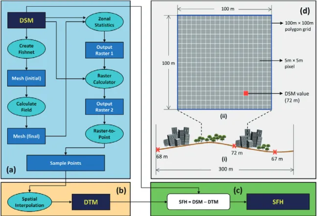
conversion of these extracted pixels to points. Fig. 1a
pre-sents a flowchart showing the automatic identification and
extraction of sample points, and the subsequent spatial interpolation of DTM and SFH extraction.
The model first creates a mesh, the size of which is de
-fined by the user (e.g., 100 m) (Fig. 1a), and each grid in
the mesh is assigned a unique identification (ID) number (calculate field). The DSM and the mesh are then used as inputs to a zonal statistics tool, which is used to generate a new raster (i.e., Output Raster 1 in Fig. 1a). In this new
raster file, if the statistical measure (statistics type) selected is ‘minimum’ (this is necessary to derive a DTM from a DSM), all pixels within a particular grid are assigned a sin-gle, common value, i.e., the lowest value among this group of pixels. The model then employs a raster calculator tool to compare the newly created raster with the DSM, to iden-tify the pixel (or pixels) in the DSM that corresponds to the lowest value found within each grid. This comparison is achieved by applying a conditional statement, i.e., Con (“DSM” == “Output Raster 1”, “DSM”), so that within each grid, if the value of pixel x in the DSM is equal to the
common value of the pixels in Output Raster 1, then pixel
x and its value is identified and extracted (i.e., Output Ras-ter 2 in Fig. 1a). In addition, within each grid, those pixels in the DSM with values not equal to the common value of the pixels in Raster Output 1 are assigned to ‘No Data’ in Raster Output 2 (Fig. 1a).
In the second step of this grid-based method, the sam-ple points are interpolated to produce a surface map – the DTM (Fig. 1b). This process of spatial interpolation is based on the principle of spatial autocorrelation, which assumes that points closer together in space are more likely to have similar values than points that are more distant (Tobler’s First Law of Geography, Tobler, 1970). There are several interpolation techniques and these are
generally classified into either deterministic or geostatis -tical. Deterministic interpolation techniques create sur-faces from measured points, based on either the extent of similarity or the degree of smoothing, while geostatistical interpolation techniques utilize the statistical properties of the measured points, quantify the spatial autocorrelation among the measured points, and account for the spatial
configuration of the sample points around the prediction
location.
Fig. 1. Semi-automatic generation of a surface feature height (SFH) map from a DSM using the grid-based method (Estoque et al., 2015). (a) identification and extraction of sample points from a DSM; (b) DTM spatial interpolation; (c) generation of a SFH map; (d)(i) a cross-section of a 300 m wide hypothetical urban landscape with topographic surface shown as a brown line; and d(ii) a 100 m grid showing the hypothetical 5 m × 5 m pixel (red) with the lowest DSM value (72 m).
Deterministic interpolation techniques include inverse distance weighting (IDW), radial basis functions (RBF), natural neighbor, trend, spline, global polynomial inter-polation (GPI), and local polynomial interinter-polation (LPI); geostatistical interpolation techniques include kriging and its variants e.g., simple, ordinary, universal, and empiri-cal Bayesian. Details of these techniques can be found in literature (e.g. Mitas and Mitasova, 1999; Childs, 2004; EPA, 2004; Wong et al., 2004; Li and Heap, 2008; Sun et al., 2009; Krivoruchko, 2012; Arun, 2013; see also ES-RI’s documentation – http://desktop.arcgis.com).
To illustrate this, Fig. 1d(i) shows a 300 m wide cross-section of a hypothetical urban landscape. In this
figure, the landscape is segmented into three parts, each
measuring 100 m wide, which corresponds to a 100 m grid. Fig. 1d(ii) shows the pixel with the lowest DSM value within the 100 m grid (i.e., red pixel with a value of 72 m). Once the model is run, this pixel is identified and
extracted, and serves as the representative sample pixel for the grid where it is located. It should be noted that two
or more pixels with the same value can be identified and
extracted within each grid, particularly if the ‘pixel type’
of the input DSM file is ‘integer’.
3. Application: Validation of ALOS PRISM DSM-de-rived surface feature height (SFH)
3.1. Extracting SFH
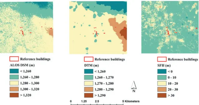
In this study, the SFH data for the six test sites were derived from ALOS PRISM DSMs provided by JAXA (Figs. 2-7). These DSMs had a spatial resolution of 5 m, and were expressed based on the ellipsoid. This study fo-cused only on the SFH of buildings.
The grid-based method (Estoque et al., 2015) was used to extract the SFH data (Fig. 1). Various grid sizes were tested for sample points identification and extraction. For the larger and denser cities of Tokyo, Beijing and Shanghai, 200 m-300 m grids were considered the most appropriate, while for the smaller and less dense cities of Surabaya, Tsukuba and Lusaka, 100 m-200 m grids were most appropriate. The results presented in this paper are all based on 200 m grids.
Following identification and extraction of the sample points for each test site (Fig. 1a), a DTM map for each site was produced through spatial interpolation (Fig. 1b) using the Empirical Bayesian Kriging (EBK) technique (Krivoruchko, 2012). The interpolated DTM maps were set to the same spatial extent and resolution as the ALOS PRISM DSMs. The derived DTM maps were then sub-tracted from their respective ALOS PRISM DSM source maps (Fig. 1c). This process resulted in six SFH maps, one for each test site (Figs. 2-7).
Validating ALOS PRISM DSM-derived surface feature height: Implications for urban volume estimation 3.2. Validating extracted SFH
To validate the derived SFH maps, sample buildings constructed prior to the capture dates of the ALOS PRISM DSM maps (Figs. 2-7), but still in existence at the time of the study, were used. Prospective sample buildings were
identified taking into account two factors: (1) rooftop com-plexity (buildings with less complex rooftops were pre-ferred); and (2) building height (only buildings with height
information were used). In this paper, building height is referred to as recorded building height (RBH). Sources of information on building height included The Global Tall Building Database of the Council on Tall Buildings and Urban Habitat (CTBUH) (www.skyscrapercenter.com; www.ctbuh.org). The polygon outline of these buildings was manually digitized and zonal analysis was performed to extract the maximum SFH values within each building
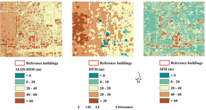
Fig. 3. ALOS PRISM DSM and derived DTM and SFH maps for the Beijing test site. The DSM map was captured on October 25, 2010.
polygon. Finally, the RBH values were compared with the maximum SFH values for each test site by calculating the root-mean-square error (RMSE).
3.3. Validation results
Fig. 8 shows the results of the validation process, based on a comparison of the derived SFH data and the
RBH data for each test site. The results showed that Bei-jing had the highest RMSE at 81 m (n = 25), followed by Tokyo at 47 m (n = 30) (Fig. 8). Conversely, Tsukuba had the lowest RMSE at 7 m (n = 30), followed by Surabaya at 11 m (n = 37). Shanghai (n = 30) and Lusaka (n = 14) both had a RMSE of 30 m (Fig. 8).
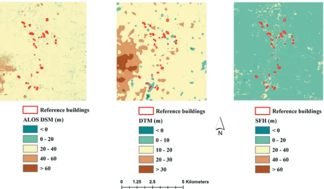
Fig. 5. ALOS PRISM DSM and derived DTM and SFH maps for the Surabaya test site. The DSM map was captured on July 17, 2010.
Validating ALOS PRISM DSM-derived surface feature height: Implications for urban volume estimation
4. Discussion
RMSE values closer to zero indicate higher accuracy or better one-to-one correspondence between the ALOS PRISM DSM-derived SFH data and the RBH data. The results showed that the datasets with the highest accuracy were from the Tsukuba and Surabaya test sites, with a RMSE of 7 m and 11 m, respectively (Fig. 8). Assuming
one building floor is equal to 3 m, this range of error ap
-proximated to between 2 and 4 building floors. However,
the other test sites had much higher RMSE values (30 m-81 m) (Fig. 8), which translated to between 10 and 27
building floors. The results also indicate that the accuracy
of the derived SFH maps varied between buildings within a test site and also between test sites (Fig. 8).
In a previous urban volume study using ALOS PRISM DSM (i.e., a “stacked DSM” across the years 2006-2011) (Estoque et al., 2015), the assessment of the results was done through visual comparison of the derived urban vol-ume map with corresponding Google Earth imagery. This present study advances the evaluation of the ALOS PRISM DSMs in the context of urban volume estimation through a more detailed and rigorous assessment. In addition, the ALOS PRISM DSMs used in this study were not “stacked data”, but rather each DSM (one per test site) was captured in a single time point (see Figs. 2-7). The resulting RMSE values produced by comparing the SFH and RBH data depended on the accuracy of these two input variables. Notwithstanding this, the derived SFH data was
consid-ered to have had more influence on the validation results
than the RBH data. This is due to errors in the SFH data attributed to two sources, namely the grid-based method
applied and the original DSMs used. Factors that can influ -ence the outcomes of the grid-based approach include the method of spatial interpolation and the size of the grid used to extract sample points for use in the spatial interpolation (as described in Section 2, there are a number of interpola-tion methods available). In this study, the selecinterpola-tion of the EBK interpolation method was based on previous studies (Krivoruchko, 2012; Estoque et al., 2015).
In a denser urban landscape, i.e., with more buildings and less open space, larger grid sizes (e.g., 300 m rather than 100 m) may be more appropriate. Larger grids in-crease the likelihood that pixels with the lowest DSM val-ue lie in an open space (a topographic space) and not on top of small buildings or similar structures. Conversely, smaller grid sizes may be more appropriate in less dense urban landscapes with more open spaces. Smaller grid sizes can also result in more detailed DTM maps. Howev-er, the selection of appropriate grid sizes can be challeng-ing because the physical characteristics (e.g. density of development) of urban landscapes can vary considerably across cities. Within a single city, the density of urban de-velopment can also vary across the city’s whole landscape (e.g., along the urban-rural gradient). In this study, grid sizes ranging between 100 m and 300 m were considered appropriate for the six test sites, based on RMSE values derived during the testing of various grid sizes. However, since the difference between RMSE values was small, the study used a 200 m grid size for all the test sites. A self-adaptive algorithm that can change grid size based on urban characteristics could present a possible future development of the grid-based method.
The accuracy of the DTM maps derived from the grid-based method and the resulting SFH maps also rely on the accuracy of the source DSMs themselves. If the DSM values of the selected pixels or points used in the DTM spatial interpolation are inaccurate (Fig. 1a) then the re-sulting DTM and SFH maps (Figs. 1b and 1c) will also be inaccurate. In this study, there was evidence to indicate that the ALOS PRISM DSMs used to derive the DTM and SFH maps had limitations. Based on the structure of the ALOS PRISM DSM data used in this study, the DSM value of a pixel occupied by a building equaled the sum of the build-ing height and the ellipsoidal height. Here, the ellipsoidal height equaled the difference between the ellipsoid and the topographic surface. Thus, it is logical to assume that the DSM values of pixels occupied by buildings should be greater than the heights of the buildings themselves (i.e., DSM > RBH). However, based on the comparison of the SFH data (maximum value within a building polygon) and RBH data, this was not always the case, with many build-ings in Tokyo, Beijing and Shanghai exhibiting RBH > DSM. It should be noted that both the datasets (DSM and RBH) were independent of the derived DTM maps,
mean-ing that they were not influenced by the grid-based method.
The validation results also indicate that derived SFH
values were more accurate for buildings with RBH of < 100 m (Fig. 8). SFH values for smaller and less dense cities with lower buildings, such as Tsukuba and Surabaya, have smaller RMSE and greater accuracy. The ALOS PRISM DSMs appeared to have failed to capture most high-rise buildings (> 100 m). Visual comparison of the ALOS PRISM DSMs and corresponding Google Earth imagery showed that some high-rise buildings were not visible or distinguishable from the ALOS PRISM DSMs. As of writ-ing, the possible causes of these observed inaccuracies or errors in the ALOS PRISM DSMs are still unclear. There-fore, it is recommended that the JAXA ALOS PRISM DSM products are reassessed, especially for urban areas, so that uncertainties in urban volume estimation can be
re-duced. Our observations and findings contribute to the val -idation of the ALOS PRISM DSMs (Takaku and Tadono 2009; Takaku et al. 2016). Taking into account the overall pattern of errors in building height (Fig. 8), it is considered that UBV is likely to be underestimated if determined us-ing the derived SFH maps.
5. Conclusions
The purpose of this study was to examine the reliability and potential of ALOS PRISM DSM data for SFH
extrac-Fig. 8. Scatter plots of the RBH data and ALOS PRISM DSM-derived SFH data across the six test sites. For each scatter plot, the RMSE and number of sample buildings used in the validation are stated.
Validating ALOS PRISM DSM-derived surface feature height: Implications for urban volume estimation
tion by validating six sets of SFH data extracted from 5 m ALOS PRISM DSMs and discuss the implications of the results to urban volume estimation. We conclude that: (1) across the six test sites, the RMSE of the SFH data ranged from 7 m (Tsukuba) (approximately 2 building floors) to 81 m (Beijing) (approximately 27 building floors); (2) the SFH data for lower buildings (e.g., RBH < 100 m) and for smaller and less dense cities were more accurate than for high-rise buildings (e.g., RBH > 100 m) and for larger and denser cities; and (3) the ALOS PRISM DSMs appeared to have failed to capture most high-rise buildings (> 100 m).
The factors that may have influenced the accuracy of
the derived SFH maps included the size of grid used in the grid-based method, the grid-based method itself, and the interpolation method used to derive the DTM maps. The RBH data may also have contained errors (the scale
of error was not quantified in this study) that could have
influenced the validation results.
In addition, there was evidence of inaccuracy within the ALOS PRISM DSMs themselves, as some buildings had RBH > DSM. As such errors in the ALOS PRISM DSM-derived SFH data could have a profound effect on urban volume estimation, it is recommended that the ALOS PRISM DSM products used be reassessed and improved if necessary. Other DTM generation methods could also be tested.
Acknowledgements
This study was supported by JSPS Grant-in-Aid for Challenging Exploratory Research 16K12816, for Scien-tific Research (A) 16H01830, and ALOS Research and Application Project of EORC, JAXA (6th RA, Geography, No3085). The authors wish to acknowledge Dr. Takeo Ta-dono, JAXA, for his valuable advice and for providing the ALOS datasets used.
References
Arefi, H., d’Angelo, P., Mayer, H. and Reinartz, P. (2011):
Iterative approach for efficient digital terrain model
production from CARTOSAT-1 stereo images. Jour-nal of Applied Remote Sensing, 5, 1–19.
Arun, P.V. (2013): A comparative analysis of different DEM interpolation methods. The Egyptian Journal of Remote Sensing and Space Sciences, 16, 133–139. Beumier, C. and Idrissa, M. (2015): Deriving a DTM
from a DSM by uniform regions and context. EAR-SeL eProceedings, 14, 16–24.
Bremer, M., Mayr, A., Wichmann, V., Schmidtner, K. and Rutzinger, M. (2016): A new multi-scale 3D-GIS-ap-proach for the assessment and dissemination of solar income of digital city models. Computers,
Environ-ment and Urban Systems, 57, 144–154.
Childs, C. (2004): Interpolating surfaces in ArcGIS spa-tial analyst. ArcUser, 32–35.
Enßle, F., Heinzel, J. and Koch, B. (2014): Accuracy of vegetation height and terrain elevation derived from ICESat/GLAS in forested areas. International Jour-nal of Applied Earth Observation and Geoinforma-tion, 31, 37–44.
EPA (Environmental Protection Agency, USA) (2004):
Developing spatially interpolated surfaces and esti-mating uncertainty. EPA, NC, USA, 159 p.
Estoque, R.C. and Murayama, Y. (2016): Quantifying landscape pattern and ecosystem service value changes in four rapidly urbanizing hill stations of Southeast Asia. Landscape Ecology, 31, 1481–1507. Estoque, R.C., Murayama, Y., Tadono, T. and Thapa, R.B.
(2015): Measuring urban volume: geospatial tech-nique and application. Tsukuba Geoenvironmental Sciences, 11, 13–20.
Hecht, R., Meinel, G. and Buchroithner, M.F. (2008): Es-timation of urban green volume based on single-pulse LiDAR data. IEEE Transactions on Geoscience and Remote Sensing, 46, 3832–3840.
Holtier, S., Steadman, J.P. and Smith, M.G. (2000): Three-dimensional representation of urban built form in a GIS. Environment and Planning B: Planning and Design, 27, 51–72.
Huang, Y., Yu, B., Zhou, J., Hu, C., Tan, W., Hu, Z. and Wu, J. (2013): Toward automatic estimation of urban green volume using airborne LiDAR data and high resolution remote sensing images. Frontiers of Earth Science, 7, 43–54.
Kabolizade, M., Ebadi, H. and Mohammadzadeh, A. (2012): Design and implementation of an algorithm for automatic 3D reconstruction of building models using genetic algorithm. International Journal of Applied Earth Observation and Geoinformation, 19, 104–114.
Koomen, E., Rietveld, P. and Bacao, F. (2009): The third dimension in urban geography: the urban-volume ap-proach. Environment and Planning B: Planning and Design, 36, 1008–1025.
Krauss, T., Arefi, H. and Reinartz, P. (2011): Evaluation of selected methods for extracting digital terrain models from satellite born digital surface models in urban areas. International Conference on Sensors and Models in Photogrammetry and Remote Sensing (SMPR 2011), pp. 1–7.
Krivoruchko, K. (2012): Empirical Bayesian kriging: implemented in ArcGIS geostatistical analyst. ESRI, Redlands, CA, USA.
Li, J. and Heap, A.D. (2008): A review of spatial interpo-lation methods for environmental scientists. Geosci-ence Australia, Canberra, Australia, 137 p.
Meng, X., Wang, L., Silván-Cárdenas, J.L. and Currit, N. (2009): A multi-directional ground filtering algorithm
for airborne LIDAR. ISPRS Journal of Photogram-metry and Remote Sensing, 64, 117–124.
Mitas, L. and Mitasova, H. (1999): Spatial interpolation. In Longley, P., Goodchild, M., Maguire, D. and Rhind, D., eds., Geographical Information Systems: Principles, Techniques, Management and Applica-tions, vol. 1. Wiley, London, pp. 481–492.
Neuenschwander, N., Hayek, U.W. and Grêt-Regamey, A. (2014): Integrating an urban green space typology into procedural 3D visualization for collaborative planning. Computers, Environment and Urban Sys-tems, 48, 99–110.
Perko, R., Raggam, H., Gutjahr, K.H. and Schardt, M. (2015): Advanced DTM generation from very high resolution stereo images. ISPRS Annals of the Photo-grammetry, Remote Sensing and Spatial Information Sciences, II-3, 165–172.
Priestnall, G., Jaafar, J. and Duncan, A. (2000): Extract-ing urban features from LiDAR digital surface mod-els. Computers, Environment and Urban Systems, 24, 65–78.
Santos, T., Rodriguez, A.M. and Tenedorio, J.A. (2013). Characterizing urban volumetry using LiDAR data.
International Archives of the Photogrammetry, Re-mote Sensing and Spatial Information Sciences, XL-4, 71–75.
Sun, Y., Kang, S., Li, F. and Zhang, L. (2009): Compar-ison of interpolation methods for depth to ground-water and its temporal and spatial variations in the Minqin oasis of northwest China. Environmental Modelling & Software, 24, 1163–1170.
Takaku, J. and Tadono, T. (2009). PRISM on-orbit ge-ometric calibration and DSM performance. IEEE Transactions on Geoscience and Remote Sensing,
47(12), 4060–4073.
Takaku, J., Tadono, T., Tsutsui, K. and Ichikawa, M. (2016). Validation of 'AW3D' global DSM generated from ALOS PRISM. ISPRS Annals of the Photo-grammetry, Remote Sensing and Spatial Information Sciences, Volume III-4, 2016, XXIII ISPRS Con-gress, 12–19 July 2016, Prague, Czech Republic. Tian, J., Krauss, T. and Reinartz, P. (2014): DTM
gener-ation in forest regions from satellite stereo imagery.
The International Archives of the Photogrammetry, Remote Sensing and Spatial Information Sciences,
XL-1, 401–405.
Tobler, W.R. (1970): A computer movie simulating urban growth in the Detroit Region. Economic Geography,
46, 234–240.
Wong, D.W., Yuan, L. and Perlin, S.A. (2004): Compar-ison of spatial interpolation methods for the estima-tion of air quality data. Journal of Exposure Analysis and Environmental Epidemiology, 14, 404–415. Yong, Z. (2001): A study on remote sensing methods
in estimating urban built-up volume ratio based on aerial photographs. Progress in Geography, 20, 378– 383.
Received 21 September, 2017 Accepted 2 November, 2017