Hidden Markov Model-Based
Speech Enhancement
Akihiro Kato
A thesis submitted for the Degree of Doctor of Philosophy
University of East Anglia
School of Computing Sciences
24, May, 2017
This copy of the thesis has been supplied on condition that anyone who consults it is understood to recognise that its copyright rests with the author and that use of any information derived there-from must be in accordance with current UK Copyright Law. In addition, any quotation or extract must include full attribution.
3
Abstract
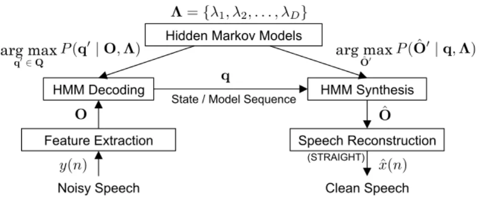
This work proposes a method of model-based speech enhancement that uses a network of HMMs to first decode noisy speech and to then synthesise a set of features that enables a speech production model to reconstruct clean speech. The motivation is to remove the distortion and residual and musical noises that are associated with conventional filtering-based methods of speech enhancement.
STRAIGHT forms the speech production model for speech reconstruction and re-quires a time-frequency spectral surface, aperiodicity and a fundamental frequency con-tour. The technique of HMM-based synthesis is used to create the estimate of the time-frequency surface, and aperiodicity after the model and state sequence is obtained from HMM decoding of the input noisy speech. Fundamental frequency were found to be best estimated using the PEFAC method rather than synthesis from the HMMs.
For the robust HMM decoding in noisy conditions it is necessary for the HMMs to model noisy speech and consequently noise adaptation is investigated to achieve this and its resulting effect on the reconstructed speech measured. Even with such noise adaptation to match the HMMs to the noisy conditions, decoding errors arise, both in terms of incorrect decoding and time alignment errors. Confidence measures are developed to identify such errors and then compensation methods developed to conceal these errors in the enhanced speech signal.
Speech quality and intelligibility analysis is first applied in terms of PESQ and NCM showing the superiority of the proposed method against conventional methods at low SNRs. Three way subjective MOS listening test then discovers the performance of the proposed method overwhelmingly surpass the conventional methods over all noise con-ditions and then a subjective word recognition test shows an advantage of the proposed method over speech intelligibility to the conventional methods at low SNRs.
5
Acknowledgements
First, thanks go to Dr Ben Milner for his excellent supervision throughout my PhD at the University of East Anglia. This work would not have been possible without his support and advice. I would also like to thank Prof. Richard Harvey and Prof. Stephen Cox for their support during my doctoral research as well as their leadership of the Speech, Language and Audio Processing group in the University of East Anglia.
Thanks also go to the members in the speech lab for their kind and heart-warming support in my research and school life.
I am deeply grateful to my family in Japan for all their love. I was always able to feel their moral support during my study abroad and I would not be able to achieve this work without it.
Finally, I would also like to thank my examiners, Dr Mark Fisher of the University of East Anglia and Dr Jon Barker of the University of Sheffield, for their comments and suggestions which improved the quality of this thesis.
7
Contents
Abstract 3 Acknowledgements 5 Contents 7 List of Figures 13 List of Tables 21 Chapter 1. Introduction 23 1.1 Speech Enhancement . . . 23 1.2 Proposed Method . . . 25 1.3 Application . . . 261.4 Objective and Problems . . . 26
1.5 Contributions . . . 27
1.6 Organisation of the Thesis . . . 27
Chapter 2. Conventional Methods for Speech Enhancement 29 2.1 Introduction . . . 29
2.2 Noise Estimation . . . 30
2.2.1 VAD-Based Noise Estimation . . . 30
2.2.2 Minimum Statistics . . . 31
2.3 Filtering-Based Speech Enhancement . . . 33
2.3.1 Spectral Subtraction . . . 33
2.3.2 Wiener Filter . . . 35
2.3.2.1 Theory of Wiener Filters . . . 36
2.3.2.2 Wiener Filtering for Speech Enhancement . . . 37
2.3.3 Statistical-Model-Based Method . . . 39
2.3.3.1 Maximum-Likelihood Estimator . . . 39
2.3.3.2 Log-MMSE estimator . . . 41
2.3.4 Subspace Algorithm . . . 43
2.3.5.1 Speech Quality . . . 46
2.3.5.2 Speech Intelligibility . . . 48
2.3.5.3 Spectral Analysis . . . 48
2.4 Reconstruction-Based Speech Enhancement . . . 52
2.4.1 Corpus and Inventory-based Speech Enhancement . . . 52
2.4.1.1 System training . . . 53
2.4.1.2 Enhancement Process . . . 56
2.4.1.3 Post-processing . . . 57
2.4.2 Model-Based Speech Enhancement . . . 57
2.5 Conclusion of the Chapter . . . 58
Chapter 3. Speech Production Models 61 3.1 Introduction . . . 61
3.2 Physical Speech Production Process and Speech Signals . . . 62
3.3 Source-Filter Models . . . 65
3.3.1 Overview . . . 65
3.3.2 Linear Predictive Coding . . . 66
3.3.3 STRAIGHT . . . 71
3.4 Sinusoidal Model . . . 73
3.4.1 Basic Sinusoidal Model . . . 73
3.4.2 Harmonics Plus Noise Model . . . 76
3.5 Estimation of the Fundamental Frequency . . . 76
3.5.1 Time-Domain Analysis . . . 77
3.5.1.1 Autocorrelation Method . . . 77
3.5.1.2 Normalised Autocorrelation . . . 78
3.5.1.3 YIN Method . . . 78
3.5.2 Cepstrum and Frequency-Domain Analysis . . . 79
3.5.2.1 Cepstrum Method . . . 79
3.5.2.2 PEFAC . . . 79
3.5.3 Experimental Results and Evaluation . . . 81
3.6 Conclusion of the Chapter . . . 83
Chapter 4. Hidden Markov Model-Based Speech Enhancement 85 4.1 Introduction . . . 85
4.2 Hidden Markov Models . . . 86
4.2.1 Probability of the Observation Sequence . . . 88
4.2.2 Optimal State Sequence . . . 90
4.2.3 Training of the HMMs . . . 91
4.3 HMM decoding and Automatic Speech Recognition . . . 93
Contents 9
4.3.2 HMM Training . . . 97
4.3.3 HMM Decoding . . . 100
4.3.4 Experimental Evaluation on ASR . . . 102
4.3.4.1 Feature Vector settings . . . 102
4.3.4.2 Acoustic Model Settings for Whole-Word HMMs . . . 104
4.3.4.3 Acoustic Model Settings for Monophone HMMs . . . 108
4.3.4.4 Acoustic Model Settings for Context-Dependent Triphone HMMs . . . 111
4.3.4.5 Language Model . . . 116
4.3.4.6 Summary of the Experimental Results of ASR . . . 118
4.4 HMM-Based Speech Synthesis . . . 120
4.4.1 HMM Training . . . 120
4.4.2 Synthesis Process . . . 124
4.4.3 Experimental Evaluation on HMM-Based Speech Synthesis . . . . 127
4.4.3.1 Feature Vectors . . . 128
4.4.3.2 Whole-Word Model . . . 130
4.4.3.3 Monophone Model . . . 130
4.4.3.4 Context Dependent Triphone HMMs . . . 132
4.4.4 Summary of the Experimental Results of HMM-Based Speech Syn-thesis . . . 136
4.5 HMM-Based Speech Enhancement . . . 137
4.5.1 Feature Extraction . . . 137
4.5.2 HMM Training . . . 139
4.5.3 HMM Decoding . . . 141
4.5.4 HMM-Based Parameter Synthesis . . . 143
4.5.5 Speech Quality . . . 143
4.5.6 Speech Intelligibility . . . 145
4.6 Conclusion of the Chapter . . . 149
Chapter 5. Adaptation of Hidden Markov Models to Noisy Speech 151 5.1 Introduction . . . 151
5.2 Parallel Model Combination . . . 153
5.2.1 Mismatch Function . . . 154
5.2.2 Distribution Mapping between Gaussian and Log-Normal . . . 157
5.2.3 Unscented Transform . . . 159
5.3 Experimental Results and Analysis . . . 164
5.3.1 Feature Vectors . . . 164
5.3.2 HMM training . . . 165
5.3.4 HMM Decoding . . . 166
5.3.5 Decoding Results . . . 167
5.3.6 HMM Synthesis and Speech Reconstruction . . . 168
5.3.6.1 Speech Quality . . . 168
5.3.6.2 Speech Intelligibility . . . 170
5.4 Conclusion of the Chapter . . . 172
Chapter 6. Improvement to Hidden Markov Model-Based Speech En-hancement 173 6.1 Introduction . . . 173
6.2 Confidence Measuring and Compensation for Decoding Errors . . . 174
6.2.1 Overview of the Confidence Measure Estimation . . . 175
6.2.2 Compensation of the Unreliable Samples . . . 176
6.2.3 Experimental Results . . . 178
6.2.3.1 Accuracy of Confidence Measure and Classification . . . 178
6.2.3.2 Effectiveness of Replacement of the Samples correspond-ing to unreliable phonemes . . . 183
6.3 Refinement of HMM-Based Speech Synthesis with Global Variance . . . . 185
6.3.1 Deterioration by STRAIGHT . . . 188
6.3.2 Over-smoothing . . . 189
6.3.2.1 Global Variance . . . 189
6.3.2.2 Experimental Results . . . 191
6.4 Conclusion of the Chapter . . . 194
Chapter 7. Evaluation of the Proposed HMM-Based Speech Enhance-ment 195 7.1 Introduction . . . 195 7.2 Test Procedure . . . 197 7.2.1 Feature Extraction . . . 198 7.2.2 HMM Training . . . 199 7.2.3 HMM Adaptation . . . 200 7.2.4 HMM Decoding . . . 201
7.2.5 Speech Parameter Synthesis . . . 201
7.2.6 Confidence Measuring . . . 203 7.2.7 Speech Reconstruction . . . 204 7.3 Objective Evaluation . . . 206 7.3.1 Speech Quality . . . 206 7.3.2 Speech Intelligibility . . . 208 7.4 Subjective Evaluation . . . 209
Contents 11
7.4.1 Speech Quality . . . 209
7.4.2 Speech Intelligibility . . . 214
7.5 Conclusion of the Chapter . . . 217
Chapter 8. Conclusions and Further Work 221 8.1 Review . . . 221
8.2 Key Findings . . . 224
8.2.1 Speech Production Model and Features . . . 225
8.2.2 Unconstrained Speech Input . . . 225
8.2.3 Noise Robustness . . . 226
8.2.4 Further Impruvement in Speech Quality . . . 226
8.3 Further Work . . . 227
8.3.1 DNN-HMM . . . 227
8.3.2 Speech Production Model . . . 227
8.3.3 Non-Stationary Noise Model . . . 227
13
List of Figures
1.1 Noise filtering approach to speech enhancement. . . 24
1.2 The basic architecture of the proposed method. . . 25
2.1 Block diagram of Wiener filters. . . 36
2.2 PESQ scores of different filtering-based methods at different SNRs in a) white noise, b) babble noise. . . 47
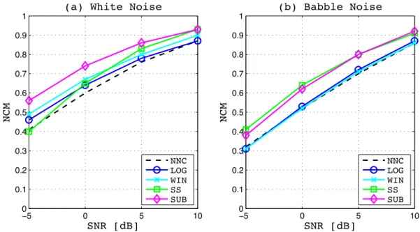
2.3 NCM scores of different filtering-based methods at different SNRs in a) white noise, b) babble noise. . . 49
2.4 Narrowband spectrograms of an utterance, “Bin Blue At E Seven Now”, spoken by a male speaker in white noise. a) shows clean speech, b) and c) show noisy speech with no enhancement at SNR of 10dB and -5dB, and d), f), h), and j) show noisy speech at SNR of 10 dB enhanced by LOG, WIN, SS and SUB while c), e), g), i) and k) show noisy speech at SNR of -5 dB enhanced by LOG, WIN, SS and SUB. . . 50
2.5 Narrowband spectrograms of an utterance, “Bin Blue At E Seven Now”, spoken by a male speaker in babble noise. a) shows clean speech, b) and c) show noisy speech with no enhancement at SNR of 10dB and -5dB, and d), f), h), and j) show noisy speech at SNR of 10 dB enhanced by LOG, WIN, SS and SUB while c), e), g), i) and k) show noisy speech at SNR of -5 dB enhanced by LOG, WIN, SS and SUB. . . 51
2.6 A framework of corpus and inventory-based speech enhancement. . . 53
2.7 Framework of model-based speech enhancement. . . 57
3.1 Overview of the human speech production model. . . 63
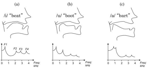
3.2 The relation between the shape of the oral and pharyngeal cavity and the frequency response of the resonance showing a) sound of /i/ in “beat”, b) sound /u/ in “boot” and c) sound /a/ in “bart”. . . 64
3.3 Time domain waveform of the utterance “bin blue at L four again” of a male speaker showing: a) the whole speech signal, b) the zoomed-in plot corresponding to the voiced segment “ue” in “blue”, c) the zoomed-in plot
corresponding to the unvoiced segment “f” in “four”. . . 64
3.4 Overview of the source-filter model. . . 65
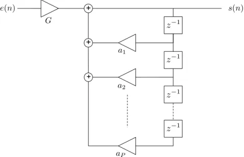
3.5 AR model forming a vocal tract filter of LPC vocoder. . . 67
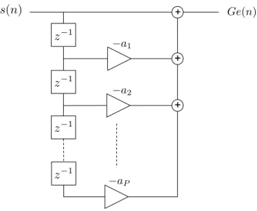
3.6 Linear prediction filter which is the inverse of the LPC model . . . 68
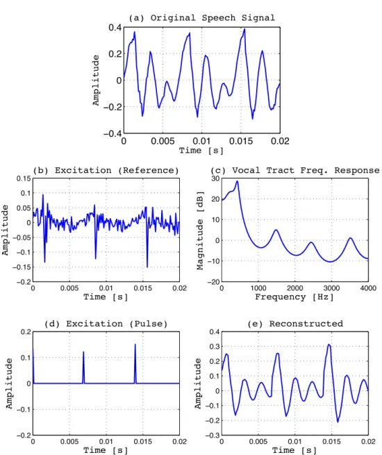
3.7 Example of the speech production with the LPC model (P = 16) showing: a) original natural speech of the sound /ue/ in “blue” uttered by a male speaker, b) the residual of the linear prediction as the reference of the excitation source, c) the frequency response of the vocal tract filter, d) pulse train used for the excitation and e) reconstructed speech with c) & d). 69 3.8 Example of the speech reconstruction with STRAIGHT showing: a) a segment of the natural speech, b) the magnitude spectrum of the vocal tract filter, c), e) and g) the excitation source where the blue line represents the sum of the periodic and noise components while the red line shows only the periodic pulse component at the group delay of 0, 0.5, and 2.0 ms respectively, d), f) and h) reconstructed speech at the group delay of 0, 0.5, and 2.0 ms respectively. . . 74
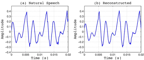
3.9 Example of the speech reconstruction with the sinusoidal model showing: a) a short-time segment of the natural speech of the sound “ue” in “blue” uttered by a male speaker and b) the reconstructed speech. . . 76
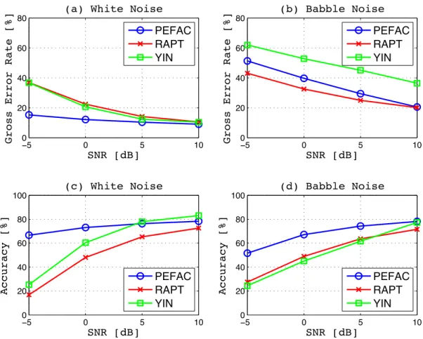
3.10 Fundamental frequency estimation performance with each methods show-ing: a) gross error rate in white noise, b) gross error rate in babble noise, c) estimation accuracy of the voiced speech in white noise and d) babble noise. . . 82
4.1 A combination of different HMM techniques to build HMM-based speech enhancement. . . 86
4.2 4 state ergodic Markov chain. . . 87
4.3 A framework of ASR. . . 93
4.4 A block diagram to extract MFCC vectors. . . 94
4.5 a) shows Mel-scale frequency warping while b) illustrates a 16 channel Mel-filterbank . . . 95
List of Figures 15
4.6 Extraction of a spectral envelope by truncating high quefrency bins of a cepstrum showing: a) spectral magnitude of speech, b) log spectral mag-nitude, c) cepstrum obtained with DCT, d) cepstrum in which quefrency bins corresponding to more than 1 ms are truncated and then padded with zeros, e) and f) log and linear spectral magnitude inverse-transformed from d). . . 98 4.7 4 state left-right HMM. . . 99 4.8 ASR accuracy with 16-state whole-word HMMs and different MFCC
set-tings in A) white noise and b) babble noise. The frame interval is 5 ms. . 103 4.9 ASR accuracy with 16-state whole-word HMMs and different MFCC
trun-cation settings in A) white noise and b) babble noise. The frame interval is 5 ms. . . 105 4.10 ASR accuracy with different whole-word HMM settings in a) white noise
and b) babble noise. The configuration of feature vectors is MFCC16-8 the frame interval of which is equal to 5 ms. . . 106 4.11 ASR accuracy with different whole-word HMM settings in a) white noise
and b) babble noise. The configuration of feature vectors is MFCC16-8 the frame interval of which is equal to 10 ms. . . 107 4.12 ASR accuracy with different whole-word HMM settings in a) white noise
and b) babble noise. The configuration of feature vectors is MFCC16-8 the frame interval of which is equal to 1 ms. . . 107 4.13 A structure of monophone models. . . 108 4.14 ASR accuracy with different monophone HMM configurations and frame
intervals. a) & b) show the ASR accuracy in white noise and babble noise with the observation vectors framed at 10 ms interval while c) & d) are results with the frame interval at 5 ms, and e) & f) show the accuracy in white noise and babble noise with the observation vectors framed at 1 ms. The configuration of feature vectors is MFCC16-8. . . 110 4.15 A structure of CD-triphone HMMs. . . 111 4.16 Tree-based model clustering . . . 113
4.17 ASR accuracy with different CD-triphone HMM configurations and frame intervals. a) & b) show the ASR accuracy in white noise and babble noise with the observation vectors framed at 10 ms interval while c) & d) are results with the frame interval at 5 ms, and e) & f) show the accuracy in white noise and babble noise with the observation vectors framed at 1 ms. The configuration of feature vectors is MFCC16-8. . . 114
4.18 ASR accuracy with different model configurations with and without the language model. The feature vector is configured as MFCC16-8 framed at 5 ms interval. . . 117
4.19 A framework of HMM-based speech synthesis for TTS. . . 120
4.20 Structure of an augmented observation vector. . . 123
4.21 Narrowband spectrograms of a) the original natural speech of “Bin Blue At E Seven Now” spoken by a male speaker, b) HMM-based speech syn-thesised by 12-state whole-word HMMs with feature vector, MFCC23-23, framed at 10 ms interval, c) HMM-based speech synthesised by 16-state whole-word HMMs with MFCC23-23 framed at 5 ms interval and d) HMM-based speech synthesised by 40-state whole-word HMMs with MFCC23-23 framed at 1 ms interval. . . 131
4.22 Fundamental frequency contours synthesised by different configurations of whole-word HMMs. . . 132
4.23 Narrowband spectrograms of a) the original natural speech of “Bin Blue At E Seven Now” spoken by a male speaker, b) HMM-based speech syn-thesised by 7-state monophone HMMs with feature vector, MFCC23-23, framed at 10 ms interval, c) HMM-based speech synthesised by 12-state monophone HMMs with MFCC23-23 framed at 5 ms interval and d) HMM-based speech synthesised by 24-state monophone HMMs with MFCC23-23 framed at 1 ms interval. . . 133
List of Figures 17
4.24 Narrowband spectrograms of a) the original natural speech of “Bin Blue At E Seven Now” spoken by a male speaker, b) HMM-based speech syn-thesised by 7-state-CD-triphone HMMs with feature vector, MFCC23-23 framed at 10 ms interval, c) HMM-based speech synthesised by 12-state-CD-triphone HMMs with MFCC23-23 framed at 5 ms interval and d) HMM-based speech synthesised by 24-state-CD-triphone HMMs with MFCC23-23 framed at 1 ms interval. . . 134
4.25 Fundamental frequency contours synthesised by different configurations of CD-triphone HMMs. . . 135
4.26 The framework of HMM-based speech enhancement. . . 138
4.27 The accuracy of model sequences in different model configurations. a) and b) show accuracy in white noise and babble noise respectively, with the feature vectors framed at 5 ms interval while c) and d) shows the results with the feature vectors framed at 1 ms interval. . . 142
4.28 PESQ scores in different model configurations comparing with the log MMSE method and no noise compensation (NNC). a) and b) show the PESQ scores of enhanced speech in white noise and babble noise respec-tively, with the feature vectors framed at 5 ms interval while c) and d) show the results with the feature vectors framed at 1 ms interval. . . 144
4.29 NCM scores in different model configurations comparing with the log MMSE method and no noise compensation (NNC). a) and b) show the NCM scores of enhanced speech in white noise and babble noise respec-tively, with the feature vectors framed at 5 ms interval while c) and d) show the results with the feature vectors framed at 1 ms interval. . . 146
4.30 Narrowband spectrograms of speech, “Bin Blue At E Six Now”, spoken by a female speaker. a) is natural clean speech. b) is contaminated with white noise at SNR of -5 dB. c) is enhanced speech with HMM-based speech enhancement using TRI N/8 configuration while d) is enhanced by the log MMSE method. . . 147
4.31 Narrowband spectrograms of speech, “Bin Blue At E Six Now”, spoken by a female speaker. a) is natural clean speech. b) is contaminated with babble noise at SNR of -5 dB. c) is enhanced speech with HMM-based speech enhancement using TRI N/8 configuration while d) is enhanced by the log MMSE method. . . 148
5.1 Distortion brought by temporal inconsistency of the states between clean and noise-matched HMMs. . . 153 5.2 Outline of parallel model combination . . . 154 5.3 An brief outline of unscented transform (M “1). . . 160 5.4 The results in decoding accuracy. a) and b) show the results in white
noise and babble noise with the feature vectors framed at 5 ms interval. c) and d) show the results in white noise and babble noise with the feature vectors framed at 1 ms interval. . . 167 5.5 Objective speech quality of the enhanced speech in terms of PESQ. a)
and b) show the results in white noise and babble noise with the feature vectors framed at 5 ms interval while c) and d) show the results using the feature vectors framed at 1 ms interval. . . 169 5.6 Objective speech intelligibility of the enhanced speech in terms of NCM.
a) and b) show the results in white noise and babble noise with the feature vectors framed at 5 ms interval while c) and d) show the results using the feature vectors framed at 1 ms interval. . . 171
6.1 The overview of the proposed method for confidence measuring. . . 175 6.2 Compensation of the samples in the output speech corresponding to
unre-liable phonemes with the corresponding samples in log MMSE. . . 177 6.3 Correct frame rate at different thresholds. a) shows the result in white
noise while b) is in babble noise. . . 179 6.4 False positive rate and false negative rate with different threshold values
at SNRs of a) -5 dB, b) 0 dB, c) 5 dB and d) 10 dB in white noise. . . 181 6.5 False positive rate and false negative rate with different threshold values
List of Figures 19
6.6 Performance of combined speech at different SNRs comparing with HMM-based speech and log MMSE. a) and b) compare PESQ scores at different SNRs in white noise and babble noise while c) and d) compare NCM scores at different SNRs in babble noise. . . 184
6.7 Narrowband spectrograms of female speech of ”Bin Blue At L Three Again“. Subplots (a), (b), (c), (d) and (e) show natural clean speech, noisy speech contaminated with white noise at SNR of -5 dB, enhanced speech with HMM-based enhancement, log MMSE and combined speech respectively. . . 186
6.8 Narrowband spectrograms of female speech of ”Bin Blue At L Three Again“. Subplots (a), (b), (c), (d) and (e) show natural clean speech, noisy speech contaminated with babble noise at SNR of -5 dB, enhanced speech with HMM-based enhancement, log MMSE and combined speech respectively. . . 187
6.9 Spectral surface of female speech, ”Bin Blue At L Three Again“, in the time-frequency domain. a), b) and c) show natural speech, HMM-based speech and HMM-based speech with the GV model respectively. . . 192
6.10 Performance of HMM-based speech with the GV model in noisy conditions compared with HMM-based speech without GV and Log MMSE. a) and b) show PESQ scores in white noise and babble noise at different SNRs while c) and d) illustrate NCM scores in white noise and babble noise. . . 193
7.1 PESQ scores of the proposed HMM-based speech enhancement at different SNRs comparing with log MMSE and the subspace method. a) shows the performance in white noise while b) shows the performance in babble noise.207
7.2 NCM scores of the proposed HMM-based speech enhancement at different SNRs comparing with log MMSE and the subspace method. a) shows the performance in white noise while b) shows the performance in babble noise.209
7.4 Test scores of the three-way MOS listening test with different configura-tions of speech enhancement. a) and b) show the scores with respect to background noise in white noise and babble noise. c) and d) show the scores focused on signal distortion while e) and f) represent overall speech quality. . . 212 7.5 The user interface of the subjective word recognition test. . . 215 7.6 Correct answer rates of the subjective word recognition test at SNRs of -5
21
List of Tables
2.1 Filtering-based methods for the tests . . . 46
4.1 Configurations of MFCC coefficients as the observation vectors without coefficient truncation. . . 102
4.2 Configurations of MFCC coefficients as the observation vectors with coef-ficient truncation. . . 104
4.3 Configurations for whole-word HMMs. . . 105
4.4 Added configurations for the tests with 1 ms-framed feature vectors. . . . 106
4.5 Configurations for monophone HMMs. . . 109
4.6 An Example of the questions at nodes of the decision tree. . . 112
4.7 Configurations for CD-triphone HMMs. . . 113
4.8 A summary of the best configurations for each ASR experiments . . . 115
4.9 Test configurations for the language model evaluation . . . 116
4.10 Configurations of the feature vectors. . . 128
4.11 Average PESQ scores of the synthesised speech with 16-state whole-word HMMs and different feature vector configurations framed at 5 ms interval. 129 4.12 Configurations of the whole-word HMMs for different frame interval. . . . 130
4.13 Configurations of the monophone HMMs for different frame interval. . . . 131
4.14 Configurations of the CD-triphone HMMs for different frame interval. . . 132
4.15 PESQ scores of synthesised speech in different model configurations. The feature vector configuration is MFCC23-23. . . 136
4.16 The configuration of the feature vectors for the test. . . 138
4.17 Model configurations. . . 140
5.1 Configurations of the acoustic features. . . 164
5.2 Model configurations for the tests with feature vectors framed at 5 ms interval. . . 165
5.3 Model configurations for the tests with feature vectors framed at 1 ms interval. . . 166
6.1 Evaluation of the decision. . . 177 6.2 PESQ and NCM scores of speech reconstructed by STRAIGHT from
nat-ural speech parameters and HMM-based speech parameters . . . 189 6.3 PESQ and NCM scores of HMM-based speech with and without the GV
model. . . 191
7.1 The common configuration of HMMs and acoustic features for the tests. . 196 7.2 Configurations of HMM-based speech enhancement for the tests. . . 197 7.3 PESQ scores at SNRs of 10 dB, 5 dB, 0 dB and -5 dB in white noise and
babble noise . . . 206 7.4 NCM scores at SNRs of 10 dB, 5 dB, 0 dB and -5 dB in white noise and
babble noise . . . 208 7.5 Subjective listening scores focused on background noise at SNRs from -5
dB to 10 dB in white noise and babble noise. . . 211 7.6 Subjective listening scores focused on signal distortion at SNRs from -5
dB to 10 dB in white noise and babble noise. . . 211 7.7 Subjective listening scores as the overall grade of speech at SNRs from -5
dB to 10 dB in white noise and babble noise. . . 211 7.8 Pairwise p-values of the algorithms over all SNR conditions. . . 214 7.9 Correct answer rates of the subjective word recognition test at SNRs of -5
dB and 0 dB in white noise and babble noise. . . 216 7.10 Pairwisep-values of the algorithms over all SNR conditions. . . 218
23
Chapter 1
Introduction
This chapter first introduces the area of speech enhancement and clarifies problems that need to be addressed. The proposed method, which is a new approach to speech en-hancement, is then introduced followed by its target applications. The objective of the research, main problems to achieve it and contributions to the research area are then clarified, and finally, the organisation of the thesis is explained.
1.1
Speech Enhancement
Speech enhancement is concerned with improving some perceptual aspects of speech that had been degraded by noise or other factors, e.g. channel distortion, packet loss and echo [1]. The focus on this work is noise in speech, which causes two main effects on the perception of speech. Firstly, the auditory perception about the quality of the speech signal is deteriorated and secondly, intelligibility of speech is affected. Such degradation of speech quality and intelligibility brings the potential of increasing listener fatigue and misunderstanding during communication and thus, techniques for speech enhancement are highly desirable.
Degradation of speech by noise occurs when the source of a speech signal is affected by noise or when noise exists on communication channels. Such a situation is very com-mon in voice communication systems, and this phenomenon is mathematically modelled as
where xpnq,dpnq and ypnq represent a discrete-time domain signal of speech, noise and
degraded noisy speech respectively, and ndenotes a discrete-time index. Therefore, the most intuitive approach to speech enhancement is to identify unknown dpnq from ypnq
and then to remove it fromypnq. However, it is not possible to identify the exact sequence
ofdpnq as long as the only accessible information isypnq, and thus, a variety of methods
to obtain an estimate of noise, ˆdpnq, instead ofdpnq have been proposed [1]. These often
assume noise stationarity and exploit periods of nonspeech activity inypnq. This enables
subtraction of ˆdpnq fromypnq and derives an estimate of clean speech, ˆxpnq, as
ˆ
xpnq “ypnq ´dˆpnq (1.2)
Details are discussed in Chapter 2 but this works as a noise filter of speech as shown in Figure 1.1, and it is explicit that residual noise is left in ˆxpnq when ˆdpnq is underesti-mated. Conversely, when ˆdpnq is overestimated, the speech signal is distorted and it may further reduce speech intelligibility [2]. There are many alternative methods based on
y(n) Noise Estimator ˆ x(n) ˆ d(n)
+
+ -Figure 1.1: Noise filtering approach to speech enhancement.
this filtering approach to speech enhancement, e.g. spectral subtraction, Wiener filtering, statistical model-based methods and subspace algorithms [1]. As evaluated in Chapter 2, although these methods have shown effectiveness to suppress noise in conditions with rel-atively high signal to noise ratio (SNR), performance falls at low SNRs such as 0 dB and below. Therefore this work proposes a novel approach that moves away from the filtering methods to achieve significant improvement to performance at low SNRs in stationary and non-stationary noise.
Additionally, to acquire additional information to estimate ˆdpnq from ypnq, various
approaches have been proposed, for example, multi-channel speech enhancement uses multiple microphones to enhance ypnq into a multiple dimensional signal in order to
1.2 Proposed Method 25
extract positional relationship between speech source and noise source and then it is exploited to enable better source separation [3]. Alternatively, audio-visual speech en-hancement uses a camera to capture visual articulators, e.g. the position of speaker’s lips, as auxiliary speech information which is independent from the SNR [4]. This the-sis, however, focuses on single-channel speech enhancement in which the only accessible information about speech is monaural noisy speech, ypnq. This represents a challenging
problem but is easier from a practical implementation point of view.
1.2
Proposed Method
The method of speech enhancement proposed in this thesis is based on a model-based approach which uses statistical parametric models of speech and a speech production model. Specifically, the statistical parametric models are realised by hidden Markov models (HMMs), which are discussed in Chapter 4, and the STRAIGHT vocoder, which is explored in Chapter 3, is adopted for the speech production model. Figure 1.2 illustrates the basic architecture of the proposed method. In this method a set of speech features are
Feature Extraction
Hidden Markov Model (HMM)
STRAIGHT Vocoder
y(n) xˆ(n)
Decoding Parameter Synthesis
Figure 1.2: The basic architecture of the proposed method.
first extracted from noisy speech and then they are decoded into a sequence of statistical models of speech parameterised as HMMs. Since the HMMs have been trained with clean natural speech, they can synthesise a set of features of noise-free speech corresponding to the decoding result. Finally, the STRAIGHT vocoder reconstructs time-domain clean speech from the synthesised parameters. The output is isolated from the noise component of the input since the speech features of the output are determined only by the statistical parameters. Therefore, the output is free from residual noise and musical noise unlike the filtering-based method shown in Figure 1.1. The statistical processes are, however,
expected to bring other types of artefacts which are attributed to, for example, decoding errors and over-smoothing, to the output speech. Furthermore, model-based approaches require an off-line process to train HMMs of speech that is not needed for filtering-based methods. Thus, the size and complexity of the system tend to increase. The detail of the method and such problems are discussed in Chapter 4 and later.
1.3
Application
The proposed method of speech enhancement is assumed to have various uses with the most representative application being mobile communication. For example, talking on a mobile phone outdoors and automatic speech recognition (ASR) in an automobile. Therefore, the proposed method needs to deal with a wide range of noise types including both stationary and non-stationary noise. This thesis evaluates the performance of speech enhancement with white Gaussian noise that represents stationary noise and babble noise (NOISEX-92) that represents non-stationary noise at SNRs from -5 dB to 10 dB by both objective and subjective tests to match the test conditions to practical applications.
1.4
Objective and Problems
The objective of this research is set as follows.
• To develop a new method of speech enhancement based on a model-based ap-proach in order to achieve better speech quality and intelligibility than conventional filtering-based approaches at low SNRs with more compact system resource than existing model-based speech enhancement.
In order to achieve the preceding purpose of the research with the proposed method, the main problems addressed in this thesis are as follows.
• To employ an speech production model and speech features for the proposed method of the model-based approach to speech enhancement
• To implement the framework which includes the processes of HMM decoding, HMM synthesis and speech reconstruction to realise the proposed method
1.5 Contributions 27
• To develop methods to obtain better HMM decoding accuracy in the proposed method
• To develop methods to detect decoding errors and methods to compensate for these erroneous frames
• To obtain better quality and intelligibility in the HMM-based speech synthesis process
1.5
Contributions
This thesis contributes to the research area of speech processing by achieving the pre-ceding objective. Simultaneously, a variety of experiments in this thesis show interesting findings in the related technologies. These also contribute to the research area in terms of both theoretical and practical development. Moreover, two conference papers have been published as interim reports during this research [5,6] and have given contributions to the research field.
1.6
Organisation of the Thesis
The remainder of this thesis is organised into seven further chapters as follows:
2. Conventional Methods for Speech Enhancement: This chapter first discusses a variety of conventional methods for speech enhancement based on the filtering approach and then evaluates performance with objective tests. The latter part of the chapter explores examples of reconstruction-based approaches to speech en-hancement which have recently been proposed.
3. Speech Production Models: The proposed method in this thesis takes a model-based speech reconstruction approach to speech enhancement. This chapter, there-fore, discusses speech production models for the process of speech reconstruction. The human physical speech production process is first described and it is then ex-tended to engineering models for speech production such as the source-filter models, the STRAIGHT vocoder and the sinusoidal model. The fundamental frequency is
a critical speech feature for the speech production model, and thus, methods to extract the fundamental frequency are then explored.
4. Hidden Markov Model-Based Speech Enhancement: The details of the pro-posed method of speech enhancement are presented in this chapter. The concept of HMMs and algorithms to apply HMMs are first discussed and then techniques for HMM decoding and HMM-based speech synthesis are explored with their applica-tion examples, including automatic speech recogniapplica-tion and text-to-speech. Finally, the proposed method of HMM-based speech enhancement is presented by com-bining the techniques of HMM-decoding, HMM-based speech synthesis and the STRAIGHT voocder.
5. Adaptation of Hidden Markov Models to Noisy Speech: Decoding accuracy in noisy speech is poor when HMMs trained with clean speech are used in the HMM decoding process. Therefore, this chapter discusses methods to adapt HMMs trained with clean speech to noisy speech in order to improve HMM decoding ac-curacy practically.
6. Improvement to Hidden Markov Model-Based Speech Enhancement:
This chapter discusses methods to improve performance of the proposed HMM-based speech enhancement. A method to compensate for decoding errors which reduce quality and intelligibility of the output speech is first presented. Then HMM-based speech enhancement using the global variance model is studied to compensate for over-smoothing in the synthesised speech parameters.
7. Evaluation of the Proposed HMM-Based Speech Enhancement: This
chap-ter reports the evaluation results of the proposed method comparing with conven-tional filtering methods after carrying out objective and subjective tests.
8. Conclusions and Further work: The final chapter first draws conclusions about the proposed method of HMM-based speech enhancement and then describes how the system may be extended.
29
Chapter 2
Conventional Methods for Speech
Enhancement
This chapter first shows overviews of the conventional methods for speech enhancement which use filtering-based approaches and then conducts practical experiments to show their performance on speech enhancement. Alternative methods to the conventional filtering-based approaches are then discussed as reconstruction-based approaches includ-ing the corpus and inventory-based method and the model-based method.
2.1
Introduction
Conventional methods for speech enhancement are normally formed as a two stage pro-cess. The contaminating noise in the speech or signal to noise ratio (SNR) of the noisy speech is estimated in the first stage and then the estimate of the noise is removed from the noisy speech by various types of filters in the second stage. Most speech enhancement methods consisting of these processes are largely categorised into spectral subtraction, Wiener filtering, statistical and subspace methods, and it is known that although these filtering-based approaches are effective to improve speech quality, those performance de-pends on the accuracy of noise and SNR estimation and, consequently, residual noise, musical noise and distortion are introduced to the enhanced speech by the estimation errors [1].
recently been proposed to reduce the artefacts produced by filtering-based methods [7]. Methods using these approaches reconstruct clean speech by estimating the acoustic features of the clean speech rather than filter the noisy speech. These methods are generally divided into two types in terms of approaches to reconstruct speech. The first uses a notion of unit selection synthesis [8], which have successfully been applied to text-to-speech (TTS) applications [9], for the speech reconstruction process in which segments of speech, e.g. phonemes, are first selected from a corpus or inventory of natural speech segments and then concatenated to synthesise clean speech while the other type of the methods utilises a speech production model, e.g. vocoders, to reconstruct clean speech. The work proposed in this thesis belongs to the latter category of the reconstruction-based approaches using the STRAIGHT vocoder for the speech production model.
The following sections first present overview of different methods for the noise es-timation. After that, methods of speech enhancement which represent filtering-based enhancement are discussed and then examined by objective tests in terms of quality and intelligibility of the enhanced speech. The topic is then moved to the reconstruction-based approaches including the corpus and inventory-reconstruction-based method which represents the methods which use a notion of unit selection synthesis for the reconstruction process, and model-based speech enhancement, which represents the methods to utilise a speech production model, that have attracted a lot of research attention recently [5, 7, 10–14].
2.2
Noise Estimation
Noise estimation is the first process of filtering-based speech enhancement. The simplest method for this process is to use voice activity detection (VAD), whose overview is presented in the first part of the section. However, VAD-based estimation cannot achieve enough accuracy in low SNR conditions [1, 15], therefore, the latter part of the section introduces a method of minimum statistics representing minimal-tracking algorithms.
2.2.1 VAD-Based Noise Estimation
VAD is a simple method to classify frames of the speech as speech-active or inactive frames. Various algorithms for VAD have been proposed and applied successfully to
2.2 Noise Estimation 31
commercial applications [1, 16–18].
The simplest way of VAD for a discrete-time speech signal,spnq, is to calculate the
energy of the mixed signal at each frame, and to classify frames whose energy is more than certain threshold,λ, as speech-active frames, otherwise the frames are categorised as speech-inactive frames. Namely, when a frame inspnq is represented as a vector as
si “ rspn`iLq, spn`iL`1q, . . . , spn` pi`1qL´1qsT pi“0,1, . . .q (2.1)
where i and L denote a frame index and a frame length, the VAD scenario gives the following classification. siPCsa as sTi si ąλ siPCsi otherwise , / . / -for@i (2.2)
whereCsaandCsi represent the cluster of active frames and the cluster of speech-inactive frames respectively.
To attain more robust performance [19] proposes another threshold σ by which all the frames inCsi are reclassified as follows.
ssi j PC1si as }ssij ´¯csi} ăσ ssi j PC1sa otherwise , / . / -for@ssij PCsi (2.3) ¯ csi“ 1 N ÿ @ssi jPCsi ssi j (2.4) where ssi
j denotes the j-th element in Csi and N is the number of elements in Csi. A cepstral analysis has also been proposed to achieve more robustness, in which the frames are classified by cepstral distances [20]. After frames in the speech are categorised as speech-active or inactive, the centroid of the spectra in the speech-inactive cluster is calculated as the estimate of the noise spectrum.
2.2.2 Minimum Statistics
The notion of noise estimation with VAD is very simple and easy for implementation but not enough accurate at low SNRs [1, 15, 16]. Moreover, it cannot track changes of
statistical features in non-stationary noise during speech-active periods. To tackle this problem, a noise estimation method using minimum statistics [21] is discussed in this section.
In the discrete-time domain, a noisy speech, ypnq, can be described as the sum of
the speech, xpnq, and noise,dpnq, as
ypnq “xpnq `dpnq (2.5)
Each signal is divided into frames with anL-length window,wpmq, for analysis as follows.
yipmq “yppq ¨wpmq xipmq “xppq ¨wpmq dipmq “dppq ¨wpmq , / / / / . / / / / -p“iL, iL`1, . . . , pi`1qL´1 m“0,1, . . . , L´1 (2.6)
whereidenotes a frame index (i“0,1, . . .). These frames are then transformed into the
frequency domain applyingN-point short-time Fourier transform (STFT) analysis.
Xipfq “ Frxipmqs (2.7)
Dipfq “ Frdipmqs (2.8)
Yipfq “ Fryipmqs (2.9)
whereF is the notation of the discrete-time Fourier transform (DFT), and f represents a frequency bin index (f “0,1, . . . , F ´1). The power spectral density (PSD) ofYipfq is approximated to the sum of the PSD ofXipfqand the PSD ofDipfqbecause the cross term ofXipfqandDipfq can be ignored as long as the speech and noise are independent each other. E“|Yipfq|2 ‰ “ E“|Xipfq|2s ‰ `E“|Dipfq|2 ‰ `2Er|Xipfq|sEr|Dipfq|s « E“|Xipfq|2s ‰ `E“|Dipfq|2 ‰ (2.10)
where the notationEr¨s denotes the statistical expectation operator.
Minimum statistics is based on a notion where short term PSD in individual fre-quency bands often decays to the noise floor even during speech active periods [21].
2.3 Filtering-Based Speech Enhancement 33
Therefore, the short term PSD of noise during a fixed observation length,K, is estimated by tracking the minimum of the periodogram|Yipfq|2 during K. However, |Yipfq|2 fluc-tuates rapidly, therefore, the estimate of PSD of noise, ˆPipfq, is tracked after applying a weighted moving average.
¯ Pipfq “ $ ’ ’ ’ ’ & ’ ’ ’ ’ % |Y0pfq|2 i“0 |Yipfq|2 i“lK pl“1,2, . . .q αP¯i´1pfq ` p1´αq|Yipfq|2 otherwise (2.11) ˆ Pipfq “ $ ’ ’ ’ ’ & ’ ’ ’ ’ % ¯ P0pfq i“0 ¯ Pipfq i“lK pl“1,2, . . .q min P¯i´1pfq,P¯ipfq ( otherwise (2.12)
whereα denotes a weight constant.
Several algorithms to optimise and compensate the preceding algorithm have also been proposed [1, 21–23].
2.3
Filtering-Based Speech Enhancement
Filtering-based algorithms for speech enhancement is a two stage process of first estimat-ing the noise, and then filterestimat-ing the speech usestimat-ing the estimated noise. Various approaches to the filtering process have been proposed and they are categorised as mentioned in Sec-tion 2.1. Each of those filtering methods are discussed in this secSec-tion.
2.3.1 Spectral Subtraction
Given noisy speech as Equations (2.5)-(2.9), a frame of the complex spectrum of the clean speech is derived in polar form.
Xipfq “ Yipfq ´Dipfq (2.13) “ |Yipfq|ejΦ i ypfq´ |D ipfq|ejΦ i dpfq (2.14)
where Φypfq and Φdpfqare the phase spectra of the noisy speech and noise respectively. As the noise spectrum is not known precisely, the noise magnitude is replaced with the
magnitude of the estimated noise spectrum at the preceding process in order to derive the estimate of the spectral magnitude of the clean speech. The phase of the clean speech is not known so it is then replaced with the phase of the noisy speech. This is motivated by the fact that phase spectra do not contribute to intelligibility as much as magnitude spectra in the condition of short time window length [24], and derives the estimate of the spectrum of the clean speech, ˆXipfq.
ˆ Xipfq “ ´ |Yipfq| ´ |Dˆipfq| ¯ ejΦi ypfq (2.15)
where|Dˆipfq|represents the estimated spectral magnitude of the noise. The time-domain enhanced speech can be obtain from Equation (2.15) by simply applying inverse Fourier transform.
Equation (2.15) is the underlying principle of the spectral subtraction and several derivative algorithms are proposed [1, 25–28]. for instance, the following applies the subtraction in the spectral power domain and simultaneously compensates overestimation or underestimation of |Dˆipfq|2. |Xˆipfq|2 “ |Yipfq|2´α|Dˆipfq|2 (2.16) “ Hipfq|Yipfq|2 (2.17) Hipfq “ 1´α |Dˆipfq|2 |Yipfq|2 (2.18)
whereαdenotes an optimised constant value to adjust the estimation. The power of the resulting spectrum can be negative value in Equation (2.16) due to overestimation of the noise. Therefore, several methods for rectification are proposed [27], for example,
$ ’ & ’ % |Xˆipfq|2 “ |Yipfq|2´α|Dˆipfq|2 |Xˆipfq|2 “ |Yipfq|2 as |Yipfq|2´α|Dˆipfq|2 ě0 otherwise (2.19)
The preceding examples of the spectral subtraction are linear process but several methods having non-linear processing are also proposed [27]. A method, for example,
2.3 Filtering-Based Speech Enhancement 35
applies weighted moving average to|Dˆipfq|2 and |Yipfq|2 before the subtraction.
|Xˆipfq|2 “ |Y¯ipfq|2´α|D¯ipfq|2 (2.20)
|D¯ipfq|2 “ λd|Dˆi´1pfq|2` p1´λdq|Dˆipfq|2 (2.21)
|Y¯ipfq|2 “ λy|Yi´1pfq|2` p1´λyq|Yipfq|2 (2.22)
whereλdandλyare weight constants. Another example is to divide the frequency domain of the speech and noise intoK sub-bands, and then replace the constant,α, in Equation (2.20) with a variableαkpiqassociated with sub-bandk(k“0,1, . . . , K´1). αkpiqvaries according to thea posteriori SNR in the corresponding sub-band of the frame.
ˆ Xk i “ Y¯ki ´αkpiqD¯ki (2.23) αkpiq “ β¨20 log10 ˆ¯ Yk i ¯ Dk i ˙ (2.24) whereXˆk
i,Y¯ki andD¯ki represent vectors consisting of the power spectrum in thek-th sub-band of|Xˆipfq|2,|Y¯ipfq|2 and|D¯ipfq|2 respectively, andβdenotes a constant determined empirically.
The spectral subtraction algorithm is based on the assumption that phase spectra do not contribute to intelligibility as much as magnitude spectra in short time frame anal-ysis as mentioned above. Recent research, however, has discovered that phase spectra can contribute to intelligibility as much as magnitude spectra even for short time du-ration when analysis-modification-synthesis parameters are properly selected [29]. This inconsistency has affected the performance of the spectral subtraction methods.
2.3.2 Wiener Filter
The spectral subtraction such as Equations (2.17) and (2.18) straightforwardly derive the spectral power or magnitude of the clean speech only from the noisy speech and the estimate of the noise. Therefore, the transfer function of the filter is not optimised by the estimation errors. The Wiener filtering approach discussed in this section optimises the transfer function of the filtering process by minimising the estimation errors in terms of mean-square error.
2.3.2.1 Theory of Wiener Filters
A Wiener filter is a linear and time-invariant filter to approximate an input signal, spnq,
to a desired signal,δpnq. Figure 2.1 shows the structure of a Wiener filter. The resultant
s(n) (n) ˆ(n) ✏(n) + + + + + + + + - h0 h1 hP 1 z 1 z 1 z 1
Figure 2.1: Block diagram of Wiener filters.
output of the filter, ˆδpnq is given as
ˆ δpnq “ P´1 ÿ k“0 hkspn´kq (2.25)
whereh0, h1,¨ ¨ ¨, hP´1 are the filter coefficients (impulse response) of Pth-order Wiener filters, and the error between the filter output and desired signal is derived as
pnq “ δpnq ´δˆpnq (2.26) “ δpnq ´ P´1 ÿ k“0 hkspn´kq (2.27)
In the frequency domain, Equation (2.27) derives
εpfq “∆pfq ´HpfqSpfq (2.28)
whereεpfq, ∆pfq,Spfq andHpfq are the Fourier transform ofpnq,δpnq,spnq andhpnq
2.3 Filtering-Based Speech Enhancement 37
the mean-square error,J.
J “E“|εpfq|2‰ “ Er∆pfq∆˚pfqs `HpfqH˚pfqErSpfqS˚pfqs
´HpfqErSpfq∆˚pfqs ´H˚pfqEr∆pfqS˚pfqs (2.29)
The derivative of J with respect to Hpfq is set equal to zero in order to minimise the
mean-square error. BJ BHpfq “ H ˚ pfqErSpfqS˚pfqs ´ErSpfq∆˚pfqs “ rHpfqErS˚ pfqSpfqs ´ErS˚ pfq∆pfqss˚ “ 0 (2.30)
Solving Equation (2.30) forHpfq, the general form of Wiener filters is derived as
Hpfq “ Er∆pfqS ˚ pfqs Er|Spfq|2s “ Pδspfq Psspfq (2.31)
wherePsspfq andPδspfqrepresent the power spectrum ofspnqand the cross-power spec-trum ofδpnq and spnq respectively.
2.3.2.2 Wiener Filtering for Speech Enhancement
In an application of speech enhancement, Equations (2.26) and (2.27) are described as
“ xpnq ´xˆpnq (2.32) “ xpnq ´ P´1 ÿ k“0 hkypn´kq (2.33)
whereypnq,xpnq and ˆxpnq correspond to the noisy speech, underlying clean speech and
the estimate of the clean speech respectively. Applying Equations (2.5) - (2.9), the frequency response of the wiener filter at i-th frame, Hipfq, is derived by referring to
Equation (2.31) as Hipfq “ Er XipfqYi˚pfqs Er|Yipfq|2s (2.34) “ ErpXipfqpXipfq `Dipfqq ˚s ErpXipfq `DipfqqpXipfq `Dipfqq˚s (2.35) “ E “ |Xipfq|2 ‰ `ErXipfqDi˚pfqs Er|Xipfq|2s `Er|Dipfq|2s `ErXipfqD˚ipfqs `ErDipfqXi˚pfqs (2.36) “ E “ |Xipfq|2 ‰ Er|Xipfq|2s `Er|Dipfq|2s (2.37)
where the cross-power spectra of the clean speech and noise are equal to zero because they are assumed to be independent each other. Hipfqcan be also expressed as a function of the a priori SNR,ξipfq. Hipfq “ ξipfq ξipfq `1 (2.38) ξipfq “ E“|Xipfq|2 ‰ Er|Dipfq|2s (2.39)
In practice, the value ofξipfq is unknown and thus, [30] proposes the following decision-directed method to estimate thea priori SNR, ˆξipfq.
ˆ ξipfq “α |Xˆi´1pfq|2 |Dˆi´1pfq|2 ` p1´αqmax ˜ |Yipfq|2 |Dˆipfq|2 ´1,0 ¸ (2.40)
where |Dˆipfq|2, |Xˆipfq|2 and α represent the estimate of the noise power spectrum ob-tained with the methods introduced in Section 2.2, the enhanced speech at frame iand a weight constant respectively. Equation (2.40) derives the estimate of thea priori SNR as a weighted moving average of the pasta priori SNR and the presenta posteriori SNR with a compensation for the case of the estimated power being negative.
In general, |Xˆi´1pfq |2 in Equation (2.40) is derived aspErXi´1pfqsq2 rather than E“|Xi´1pfq |2
‰
by a speech enhancement algorithm. This causes a bias in the estimate ofa priori SNR. Therefore, the following modification to the decision-directed approach has been recommended in order to reduce the influence of this bias [31].
ˆ ξipfq “max « α|Xˆi´1pfq| 2 |Dˆi´1pfq|2 ` p1´αq ˜ |Yipfq|2 |Dˆipfq|2 ´1 ¸ , ξmin ff (2.41)
2.3 Filtering-Based Speech Enhancement 39
whereξmindenotes the minimum value allowed forξipfq. Different approaches to estimate low-variance SNR are proposed in addition to the preceding methods [1, 32].
Equations (2.37) and (2.38) are the underlying principles to optimise Wiener filters, and several derivative algorithms have been proposed, for example, [33] generalises the Wiener filtering as the parametric Wiener filters
Hipfq “ ˆ Pi xxpfq Pi xxpfq `αPddi pfq ˙β (2.42) where Pi
xxpfq and Pddi pfq represent the power spectrum of xpnq and dpnq at i-th frame respectively, and the algorithm is parameterised byα and β.
The spectrum of the enhanced speech, ˆXipfq, is derived as
ˆ
Xipfq “HipfqYipfq (2.43)
Moreover, an iterative wiener filtering algorithm in whichHipfqis renewed by the derived enhanced speech, ˆXipfq, recursively has also been proposed for speech enhancement [1].
2.3.3 Statistical-Model-Based Method
The Wiener filters in the previous section formed an optimised linear model between the complex spectra of the noisy and clean speech in terms of mean-square error. This section has a discussion about filtering algorithms which construct nonlinear statistical models between the magnitude of the clean and noisy speech.
Various techniques to build nonlinear statistical estimators have been proposed [1], and they are largely categorised into the methods based on the maximum-likelihood (ML) approach or the Bayesian approach. The first part of this section describes the overview of the ML estimator while the latter part shows the overview of the log-MMSE estimator as a representative of the Bayesian estimators.
2.3.3.1 Maximum-Likelihood Estimator
Supposing the speech signals are under the conditions of Equations (2.5)-(2.9) and (2.14), an ML estimator is derived with the hypothesis where the probability density function (pdf) of the noisy speech spectrum,Yipfq, is parametrised by the clean speech spectrum,
Xipfq, and thus, the clean speech spectrum is estimated as follows [34].
ˆ
Xipfq “arg max Xipfq
ppYipfq;Xipfqq (2.44)
where ˆXipfq and ppYipfq;Xipfqq denote the estimate of the clean speech spectrum and the pdf of the noisy speech spectrum parameterised by the clean speech spectrum.
In the ML approach, Xipfq is assumed to be deterministic and the noise spectrum
Dipfq is assumed to be zero-mean, complex Gaussian whose real and imaginary parts have variances ofλi
dpfq{2. These assumptions give the pdf of Yipfq as
ppYipfq;|Xipfq|,Φixpfqq “ 1 πλi dpfq exp « ´|Yipfq ´ |Xipfq|e jΦi xpfq|2 λi dpfq ff (2.45)
The phase parameter is integrated to be eliminated from the parameters.
pLpYipfq;|Xipfq|q “ ż2π
0
ppYipfq;|Xipfq|,ΦixpfqqppΦixpfqqdΦixpfq (2.46)
Assuming the phase Φi
xpfq has a uniform distribution between r0,2πs, the likelihood function is derived as pLpYipfq;|Xipfq|q “ 1 πλi dpfq exp „ ´|Yipfq| 2` |X ipfq|2 λi dpfq ¨ 1 2π ż2π 0 exp » – 2|Xipfq|< ´ e´jΦi xY ipfq ¯ λi dpfq fi fldΦixpfq (2.47)
Exploiting the modified Bessel function of the first kind [34], the preceding equation is simplified as pLpYipfq;|Xipfq|q “ 1 πλi dpfq c 2π2|Xipfq||Yipfq| λi dpfq ¨exp „ ´|Yipfq|2` |Xipfq|2´2|Xipfq||Yipfq| λi dpfq (2.48)
The derivative of the log-likelihood function, logpLpYipfq;|Xipfq|q, with respect to
2.3 Filtering-Based Speech Enhancement 41
for|Xipfq|, the ML estimate of the clean spectral magnitude is derived as
|Xˆipfq| “ 1 2 „ |Yipfq| ` b |Yipfq|2´λidpfq (2.49)
As the phase spectrum of the clean speech is unknown, the phase spectrum of the noisy speech is combined with the estimate of the clean magnitude spectrum in order to obtain the complex spectrum of the enhanced speech as well as the process in the spectral subtraction. ˆ Xipfq “ |Xˆipfq|ejΦ i ypfq“ |Xˆ ipfq| Yipfq |Yipfq| (2.50) “ » – 1 2 ` 1 2 d |Yipfq|2´λidpfq |Yipfq|2 fi flYipfq (2.51) “ « 1 2` 1 2 d γipfq ´1 γipfq ff Yipfq (2.52) γipfq “ |Yipfq|2 λi dpfq (2.53)
whereγipfqrepresents the a posteriori SNR
2.3.3.2 Log-MMSE estimator
In the maximum-likelihood approach, the clean speech spectrum is assumed to be deter-ministic but unknown. This section discusses an estimator using the Bayesian approach in which the spectrum of the clean speech is assumed to be a random variable, and thea priori knowledge about the magnitude spectrum of the clean speech pp|Xipfq|q is given to the estimator. Several methods using the Bayesian approach have been proposed such as the MMSE magnitude estimator, log-MMSE estimator and maximum a posteriori (MAP) estimator [1, 35–38]. This section specifically explores the log-MMSE estimator as a representative of the Bayesian estimators which gives the best performance both objectively and subjectively in the statistical-model-based methods [1, 39].
The log-MMSE method forms a statistical model to minimises the mean-square error between the estimate and the true value of the magnitude spectrum of the clean speech
in the log-magnitude domain. ˆ Xipfq “arg min ˜ Xipfq ´ E ” plog|Xipfq| ´log|X˜ipfq|q2 ı¯ (2.54)
Thus, given the complex spectrum of the noisy speech, Yipfq, the log-MMSE estimator is derived as
log|Xˆipfq| “ Erlog|Xipfq| |Yipfqs (2.55)
|Xˆipfq| “ exppErlog|Xipfq| |Yipfqsq (2.56)
Let Zf “ logXipfq, and the moment-generating function of Zf is given in order to evaluate the conditional expectation in the preceding equation.
ΦZf|Yipfqpµq “ ErexppµZfq |Yipfqs (2.57)
“ Er|Xiµpfq| |Yipfqss (2.58)
Erlog|Xipfq| | Yipfqs can be obtained by the derivative of the moment-generating func-tion at µ“0. Erlog|Xipfq| | Yipfqs “ d dµΦZf|Yipfqpµq ˇ ˇ ˇ µ“0 (2.59) “ 1 2log E“|Xipfq|2 ‰ 1`ξipfq `1 2logνipfq ` 1 2 ż8 νipfq e´t t dt (2.60)
whereνipfq,ξipfq and γipfq are defined by
νipfq “ ξipfq 1`ξipfq γipfq (2.61) ξipfq “ E“|Xipfq|2 ‰ Er|Dipfq|2s (2.62) γipfq “ | Yipfq|2 Er|Dipfq|2s (2.63)
The log-MMSE estimator is obtained by substituting Equation (2.60) into (2.56).
|Xˆipfq| “ ξipfq 1`ξipfq exp # 1 2 ż8 νipfq e´t t dt + |Yipfq| (2.64)
2.3 Filtering-Based Speech Enhancement 43
The preceding equation shows the log-MMSE is parameterised by both a priori SNR,
ξipfq and a posteriori SNR,γipfq. Thus, the log-MMSE estimator can be expressed as
|Xˆipfq| “Gpξipfq, γipfqq |Yipfq| (2.65)
whereGpξipfq, γipfqqrepresents a gain function of the log-MMSE estimator. In practice, the value of thea priori SNR is unknown and thus, it is estimated with, for example, the decision-directed method given by Equation (2.40).
2.3.4 Subspace Algorithm
The subspace algorithms transform the noisy speech into a new space that comprises speech and noise subspaces [40, 41]. Elimination of the noise subspace can retain speech components and remove noise components. Thus, the subspace algorithms do not re-quire the noise estimation process unlike the other filtering algorithms mentioned above. However, retaining too few speech components oversmooths the speech while retaining too many components leaves residual noise.
Considering vectors representing the clean and noisy speech and noise, the noisy speech is determined with the vectors as
yi “ xi`di (2.66)
xi “ rxpn` pi´1qLq, xpn` pi´1qL`1, . . . , xpn`iL´1qsT (2.67)
yi “ rypn` pi´1qLq, ypn` pi´1qL`1, . . . , ypn`iL´1qsT (2.68)
di “ rdpn` pi´1qLq, dpn` pi´1qL`1, . . . , dpn`iL´1qsT (2.69)
where xpnq, ypnq, dpnq, i, and L denote the clean and noisy speech, noise, frame index
and frame length respectively. The clean speech vectors constitute a speech subspaceX
as anLˆM matrix.
X“ rx1,x2,¨ ¨ ¨,xMs (2.70)
Assuming the speech and noise are independent of each other,xi and di are assumed to be orthogonal. Thus, they can be decoupled fromyi by projecting yi into the subspace
by a projection matrix, P, determined by
P“XpXTXq´1XT (2.71)
For simplification, X can be decomposed by singular value decomposition (SVD) as
X“UΣVH (2.72)
whereXis assumed to be full column rank such that rankpXq “M,Uis anLˆLunitary matrix consisting of eigenvectors of XXT, V is an M ˆM unitary matrix comprising eigenvectors of XTXand Σis anL
ˆM diagonal matrix comprising the singular values
of X. Equations (2.71) and (2.72) leads to
P“UUH (2.73)
This projection matrix dividesxi and di fromyi as
xi “ UUHyi (2.74)
di “ pI´UUHqyi (2.75)
IfX is assumed not to be full rank, i.e. rankpXq “r ăM, Equation (2.72) is expressed
as X“ „ U1 U2 » — – Σ1 0 0 0 fi ffi fl » — – VH 1 VH 2 fi ffi fl“U1Σ1V H 1 (2.76)
where U1, U2, V1 and V2 areN ˆr,N ˆ pN ´rq,rˆM and pM´rq ˆM matrices respectively extracted from U and V. Σ1 is a r ˆr diagonal matrix comprising the singular values ofX. Equations (2.71) and (2.76) lead to
2.3 Filtering-Based Speech Enhancement 45
Alternatively, the following is derived exploiting the unitarity ofU.
UUH “ „ U1 U2 » — – UH 1 UH 2 fi ffi fl“U1U H 1 `U2UH2 “I (2.78)
Therefore, another projection matrix,Q, projectingyinto the noise subspace is given by
Q“I´U1UH1 “U2UH2 (2.79)
The above derives the underlying principle of the subspace algorithms for speech en-hancement as
xi “ U1UH1 yi (2.80)
di “ U2UH2 yi (2.81)
In empirical conditions, however, the speech and noise spaces are not entirely sep-arable particularly with the coloured noise, therefore, it is necessary to embed a further filtering algorithm to remove the residual noise [42].
2.3.5 Experimental Results and Analysis
Various types of the filtering-based methods are discussed above and those different ap-proaches to noise filtering bring different properties to the result of speech enhancement. It is important to understand the performance and limitations of each method prior to concluding the discussion of filtering-based speech enhancement. Therefore, this section examines the performance of filtering-based speech enhancement in noisy conditions and then evaluates the results in terms of speech quality and intelligibility objectively.
Experiments use speech from four speakers in the GRID database [43] (two males and two females) which is down-sampled to 8 kHz assuming telephony applications. From the 1000 utterances from each speaker, 200 are used for the tests. The test speech is contaminated with each of white noise and babble noise at SNRs from -5 dB to 10 dB. Then the noisy speech is first divided into 25 ms-frames with 50 % overlap by a Hamming window and then, the noise power spectrum,|Dˆipfq|2, at thei-th frame is estimated by
using VAD-based estimation after 1024 point DFT as |Dˆipfq |2 “ $ ’ ’ ’ ’ & ’ ’ ’ ’ % |Yipfq |2 i“0 α|Dˆi´1pfq |2 `p1´αq |Yipfq |2 ią0, ˆγi ă3 |Dˆi´1pfq |2 ią0, ˆγi ě3 (2.82) ˆ γi “ 10 log10 k Yipfqk2 kDˆi´1pfqk2 (2.83)
where |Yipfq|2 represents the power spectrum of the observed noisy speech at the i-th frame, andα is set equal to 0.9. After the noise estimation the noisy speech is enhanced by four types of the filtering methods in Table 2.1. The log-MMSE is based on Equation
LOG: Log MMSE WIN: Wienner Filter SS: Spectral Subtraction SUB: Subspace Algorithm
Table 2.1: Filtering-based methods for the tests
(2.64) while the Wiener filter is based on Equation (2.38), and the a priori SNR is estimated with Equation (2.40) in both methods (α“0.98). The spectral subtraction is
based on Equation (2.16) where
α“ $ ’ ’ ’ ’ & ’ ’ ’ ’ % 5 ˆγi ă ´5 1 ˆγi ą20 4 otherwise (2.84)
The subspace algorithm is based on Equation (2.80) with built-in pre-whitening [42].
2.3.5.1 Speech Quality
As mentioned in Section 1.1, speech enhancement is concerned with improving some perceptual aspect of speech degraded by noise, and noise in speech brings two main effects on perception of speech. The first is to degrade quality of speech and the second is to reduce intelligibility of speech. Therefore, speech quality and intelligibility are regarded as the most important attributes to gauge the performance of speech enhancement and have widely been used to evaluate speech signals. Speech quality generally gauges how
2.3 Filtering-Based Speech Enhancement 47
a speaker produces an utterance while speech intelligibility measures what the speaker said. These measures are attributed to many factors and the connection to the acoustic features of the speech has not been fully discovered yet [1]. Therefore, subjective listening tests, such as the mean opinion score (MOS) test to gauge speech quality and speech identifying test to measure speech intelligibility, are more reliable than objective tests to evaluate speech enhancement [44]. However, a number of objective measures have been proposed to predict the subjective measures and some of them have good correlation with subjective measures of speech quality or intelligibility. Evaluation across a range of objective measures shows that the perceptual evaluation of speech quality (PESQ) and the frequency-weighted segmental SNR (fwSNRseg) achieve the highest correlation with speech quality while the coherence speech intelligibility index (CSII) and the normalised-covariance measure (NCM) performs the best for speech intelligibility [45]. The results of the experiments in this section are objectively scored with PESQ and NCM to evaluate speech quality and intelligibility respectively.
Figure 2.2 shows the performance of the four filtering-based algorithms comparing with baseline performance given by no noise compensation (NNC) in terms of PESQ at different SNRs in white noise and babble noise. In white noise, SUB and LOG are
−5 0 5 10 1 1.2 1.4 1.6 1.8 2 2.2 2.4 2.6 2.8 3 SNR [dB] PESQ
(a) White Noise
NNC LOG WIN SS SUB −5 0 5 10 1 1.2 1.4 1.6 1.8 2 2.2 2.4 2.6 2.8 3 SNR [dB] PESQ (b) Babble Noise NNC LOG WIN SS SUB
Figure 2.2: PESQ scores of different filtering-based methods at different SNRs in a) white noise, b) babble noise.
superior to the other methods over the SNR range. Specifically, SUB shows the higherst scores at SNRs of 0 dB and -5 dB while LOG shows the best performance at SNRs of 5 dB and 10 dB. WIN performs with higher scores than SS between -5 dB and 5 dB but SS becomes higher than WIN at 10 dB.
In babble noise, however, SUB shows always the lowest of the four methods over the SNR range as opposed to LOG showing always the highest scores followed by WIN an SS respectively. This is attributed to the fact that noise and speech are not sufficiently orthogonal in babble noise, and thus, noise and speech are not transformed to the proper subspace in this condition.
As the overall evaluation in terms of PESQ, LOG shows the best performance of the four methods while the worst is SS. Superiority between WIN and SUB depends on attributes of noise. Incidentally, even the best method reduces the score below 1.6 at -5 dB in white noise and below 1.4 at -5 dB in babble noise. This implies the filtering-based methods do not show their effectiveness at low SNRs such as below 0 dB.
Comparing with NNC, the effectiveness of each method for speech enhancement in babble noise is less than the case of white noise.
2.3.5.2 Speech Intelligibility
Figure 2.3 shows the performance of the four filtering-based methods comparing with baseline performance given by NNC in terms of NCM at different SNRs in white noise and babble noise. The performance of SUB looks superior to the others as the overall evaluation, but all of the four methods reduce the score at lower SNRs and cannot retain sufficient intelligibility. For example, NCM score of SUB falls below 0.6 at SNR of -5 dB and the other methods become below 0.5 in white noise. Moreover, scores of all the methods fall far below 0.5 at -5 dB in babble noise. The general tendency of speech intelligibility of each method at different SNRs does not show significant difference from NNC.
2.3.5.3 Spectral Analysis
To give further insight into filtering-based speech enhancement, Figures 2.4 and 2.5 depict narrowband spectrograms of an utterance, “Bin Blue At E Seven Now”, spoken by a
2.3 Filtering-Based Speech Enhancement 49 −5 0 5 10 0 0.1 0.2 0.3 0.4 0.5 0.6 0.7 0.8 0.9 1 SNR [dB] NCM
(a) White Noise
NNC LOG WIN SS SUB −5 0 5 10 0 0.1 0.2 0.3 0.4 0.5 0.6 0.7 0.8 0.9 1 SNR [dB] NCM (b) Babble Noise NNC LOG WIN SS SUB
Figure 2.3: NCM scores of different filtering-based methods at different SNRs in a) white noise, b) babble noise.
male speaker in white noise and babble noise at SNRs of 10 dB and -5 dB. The figures show that large parts of spectral envelopes and harmonic information still remain among residual and musical noise after the process of each methods at SNR of 10 dB. However, at SNR of -5 dB, those are masked under residual noise or eliminated leaving musical noise especially in the frequency band above 1.5 kHz. These degradation are brought by overestimation and underestimation of the noise. The subspace method estimates the noise space on the assumption that it is orthogonal to the speech space rather than using VAD. Therefore, spectral information remains with less estimation errors even at SNR of -5 dB as long as the noise is orthogonal to the speech (i.e., white noise). However, it loses most of the de-noising function when the noise does not have orthogonality to the speech such as the case of babble noise.
The experiments show that the filtering-based methods are effective to reduce the noise at relatively high SNRs but but those performance are insufficient at low SNRs such as 0 dB and below. This brings a motivation to discuss the reconstruction-based speech enhancement as an alternative approach to the filtering-based methods.
Figure 2.4: Narrowband spectrograms of an utterance,“Bin Blue At E Seven Now”, spoken by a male speaker in white noise. a) shows clean speech, b) and c) show noisy speech with no enhancement at SNR of 10dB and -5dB, and d), f ), h), and j) show noisy speech at SNR of 10 dB enhanced by LOG, WIN, SS and SUB while c), e), g), i) and k) show noisy speech at SNR of -5 dB enhanced by LOG, WIN, SS and SUB.