An Efficient Method of Solving Lexicographic Linear Goal
Programming Problem
U.C.ORUMIE D.W EBONG
Department of Mathematics/Statistics, University of Port Harcourt, Nigeria [email protected] & [email protected]
Abstract
Lexicographic Linear Goal programming within a pre-emptive priority structure has been one of the most widely used techniques considered in solving multiple objective problems. In the past several years, the modified simplex algorithm has been shown to be widely used and very accurate in computational formulation. Orumie and Ebong recently developed a generalized linear goal programming algorithm that is efficient. A new approach for solving lexicographic linear Goal programming problem is developed, together with an illustrative example. The method is efficient in reaching solution.
Keywords: Lexicographic Goal programming, multi objective, simplex method.
1.INTRODUCTION
Multiple Objective optimizations technique is a type of optimization that handles problems with a set of objectives to be maximized or minimized. This problem has at least two conflicting criteria/objectives. They cannot reach their optimal values simultaneously or satisfaction of one will result in damaging or degrading the full satisfaction of the other(s). There is no single optimal solution in this type of optimization; rather an interaction among different objectives gives rise to a set of compromised solutions, largely known as the trade-off or non dominated or non inferior or Pareto-optimal solutions. Multiple Objective optimization consists of different problem situations, such as multiple objective linear programming (MOLP), Multiple Objective Integer Linear Programming (MOILP), and Nonlinear Multiple Objective Optimization (NMOO).
Wang et.al (1980) and Evans (1984) categorised multiple objective optimization into three as shown in Aouni and Kettani (2001). The categories are as follows;
• A priori techniques in which all decision maker preferences are specified before the solution process.
• Interactive techniques in which the decision maker preferences are elicited during the solution technique, mainly in response to their opinion of solutions generated to that point.
• A posteriori techniques where the solution process takes place first and the decision maker preferences are then elicited from the generated set of solution.
Goal programming is one of the posteriori techniques, and most commonly method for solving multiple objective decision problems. (See Sunar and Kahraman (2001)). Goal programming popularity from amongst the distance-based MCDM techniques as described by Tamize and Jones (2010) demonstrates its continuous growth in recent years as represented below;
Goal Programming as a Multi-criteria Decision Analysis Tool
Source: Tamiz M, &D. F Jones (2010) Practical Goal Programming. International Series in Operations Research & Management Science. Springer New York http://www.springer.com/series/6161.
Goal programming is used in optimization of multiple objective goals by minimizing the deviation for each of the objectives from the desired target. In fact the basic concept of goal programming is whether goals are attainable or not, an objective may be stated in which optimization gives a result which come as close as possible to the desired goals. Schniederjans and Kwaks (1982) referred to the most commonly applied type of goal programming as "pre-emptive weighted priority goal programming" and a generalized model for this type of programming is as follows: minimize: Z =
∑
−+
+ m i i i i ip
d
d
w
(
)
(1.1) s.t∑
+
−−
+=
=
n j i i i ij ijx
d
d
b
i
m
a
(
1
,
2
,...,
),
(1.2)0
,
,
i− i+≥
ijd
d
x
,w
i>
0
,(
i
=
1
,
2
,...,
m
:
j
=
1
,
2
,
3
...,
n
)
(1.3)In many situations, however, a decision maker may rank his or her goals from the most important (goal 1) to least important (goal m). This is called Preemptive goal programming and its procedure starts by concentrating on meeting the most important goal as closely as possible, before proceeding to the next higher goal, and so on to the least goal i.e. the objective functions are prioritized such that attainment of first goal is far more important than attainment of second goalwhich is far more important than attainment of third goal, etc, such that lower order goals are only achieved as long as they do not degrade the solution attained by higher priority goal. When this is the case, pre emptive goal programming may prove to be a useful tool. The objective function coefficient for the variable representing goal i will be pi. In problem with more than one goal, the
decision maker must rank the goals in order of importance.
However, a major limitation in applying GP as recorded in Schniederjans, M. J. & N. K. Kwak (1982) has been the lack of an algorithm capable of reaching optimum solution in a reasonable time. Hwang and Yoo (1981) cited a number of limitations found in existing algorithms. The purpose of this research is to present an efficient method for solving lexicographic linear goal programming problems.
The paper is organized as follows: Introduction to Preemptive Linear Goal Programming is provided in section two. The new algorithm for lexicographic goal programming and the solution description are the focus of Section three and four respectively, whereas the summary and conclusion will be presented in section five and six respectively.
2.LEXICOGRAPHIC (PREEMPTIVE) LINEAR GOAL PROGRAMMING (LLGP)
The basic purpose of LLGP is to simultaneously satisfy several goals relevant to the decision-making situation. To this end, a set of attributes to be considered in the problem situation is established. Then, for each attribute, a target value (i.e., appraisal level) is determined. Next, the deviation variables are introduced. These deviation variables may be negative or positive (represented by di-and di+ respectively). The negative deviation variable, di- , represents the quantification of the under-achievement of the ith goal. Similarly, di+ represents the
quantification of the over-achievement of the ith goal. Finally for each attribute, the desire to overachieve (minimize di-) or underachieve (minimize di+ ), or satisfy the target value exactly (minimize di-+ di+ ) is
articulated. And finally, the deviational variables prioritized in order of importance.
The general algebraic representation of lexicographic linear goal programming is given as
(
− +)
(
− +)
(
− +)
=
p
d
d
p
d
d
p
kd
kd
kz
lexi
min
(
1 1,
1,
2 2,
2,
...,
,
(2.1) S.t∑
+
−−
+=
=
n j i i i ij ijx
d
d
b
i
m
a
(
1
,
2
,...,
),
(2.2)0
,
,
i− i+≥
ijd
d
x
,w
i>
0
,(
i
=
1
,
2
,...,
m
:
j
=
1
,
2
,
3
...,
n
)
(2.3)The model has k priorities, m objectives and n decision variables. pi is the ordered i
th
priority levels of the deviational variables in the achievement function. The priority structure for the model is established by assigning each goal or a set of goals to a priority level, thereby ranking the goals lexicographically in order of importance to the decision maker. This is known as lexicographic GP (LGP), as introduced by Ijiri (1965), and developed by Lee (1972) , and Ignizio (1976). This was modified by [11], [12], [13], [14], and [15].Priorities do not take numerical value, but simply a suitable way of indicating that one goal is more important than another.
3.THE NEW ALGORITHM FOR LEXICOGRAPHIC GOAL PROGRAMMING (LGP)
The procedure utilizes Orumie and Ebong (2011) initial table with modifications as shown below, together with the inclusion of hard constraints. The procedure considers goal constraints as both the objective function and constraints. The objective function becomes the prioritized deviational variables and solves sequentially starting from the highest priority level to the lowest. It starts by not including the deviational variable columns that did not appear in the basis on the table, but developed when necessary since di+= - di-.
TABLE 1.1 INNITIAL TABLE OF THE NEW ALGORITM
Variable in basis with pi . CB X1 X2 … Xn S d1(v) d2(v) . . .dt(v) Solution value bi. R.H.S
a11 a12. … a1n s1 c11(v) c11(v) . . . c1t(v) b1
a21 a22 … a2n s2 c21(v) c22(v) . . .c2t(v) b2
am1 am2 … amn sm cm1(v) cm2(v). . . cmt(v) bm
Consider the Preemptive Linear Goal programming model. The formulation for n variables, m goal constraints, t deviational variables in z and L preemptive priority factors is defined below.
)
1
.
3
(
}
,...,
2
,
1
{
)
,
(
min
z
p
d
d
for
k
i
m
lex
t l k i i k t t⊂
⊂
=
∑
− + (3.1) such that i i i m i j ijx
d
d
b
a
+
−−
+=
∑
(3.2) i n j j ijx
b
a
≤
∑
(3.3)x
ij,
d
i−,
d
i+≥
0
(3.4) for(
i
=
1
,
2
,...,
m
:
j
=
1
,
2
,
3
...,
n
)
where pk= kth priority factor k= 1,2, . . .L,
)
,
(
+ − k k i id
d
are set of deviational variables in z with the priorities attached to them.0
,
,
i+ i−≥
jd
d
x
i
=
1
,...,
m
,
j
=
1
,...
n
,
Let pk be the kth priority level, then; the algorithm; Step 1. Initialization:
Set k
←
1 i.e set the first priority k=1Step 2. Feasibility:
If
b
i = 0 for i=1,2,. .., m, go to Step 8. i.e if all the rhs=0 {solution optimal} Setb
i←
b
i for I =1,2,..., m. i.e take absolute value of the rhs {ensure feasibility}Step 3. Optimality test:
If
g
hj≤ 0 for all j≠
pivot
column
,h
∈
i
kgo to Step 7. {all coefficients of priority rowh
non positive ,so is satisfied}.Step 4. Entering variable:
Entering variable is the variable with highest positive coefficient in the row
g
h.,
h
∈
{
1
,
2
,
L
}
for the − +t
t i
i
k
d
d
p
(
,
) rows of the objective function which does not violate priority condition. i.e ifg
h.,
h
∈
{
1
,
2
,
L
}
is the highest coefficient, but has been previously satisfied or more important than the leaving variable under consideration, then consider the next higher value on the same row, otherwise go to step 7. (The priority attached to the entering variable should be placed alongside with it into the basis).In case of ties {
s
hj
hj
g
g
,.
.
.,
>
0
:
min
q q hj hj i hg
g
b
is maximumj
q:
q
=
1
,...,
s
{ties in the priority rows }
Step 5. Leaving variable:
If
y
0 is the column corresponding to the entering variable in Step 4, then the leaving variable is the basic variable with minimum
=
>
i
m
g
g
b
y y i:
0
,
1
,
2
,...
0 0 . . { 0 .yg
is the pivot column}.In case of ties, the variable with the smallest right hand side leaves the basis.
Step 6. Interchange basic variable and non basic variable:
Perform Gauss Jordan row operations to update the table. If is still in the basis (CB), go to
Step 3.
Step 7. Increment process:
Set k
←
k +1.If k ≤ L, go to Step 3. Satisfied priority will not reenter for the lesser one to leave, instead variable with the next higher coefficient enters the basis.Step 8. Solution is optimal when:
i.) The coefficient of the priority rows are all negative or zero ii.) The right hand sides of the priority rows are all zero iii.) The priority rows are satisfied.
The optimal solution is the value
p
k(
d
i+,
d
i−)
in the objective function as appeared in the last iteration table.i.e. The value of the achievement function becomes a vector of priority levels in the optimal values in the final tableau.
Note : Just as in the method of artificial variables, a variable of higher or equal priority that has been
satisfied should not be allowed to re-enter the table. In this case the next higher coefficient of hj
g
will be considered.4.SOLUTION OF ILLUSTRATIVE EXAMPLE
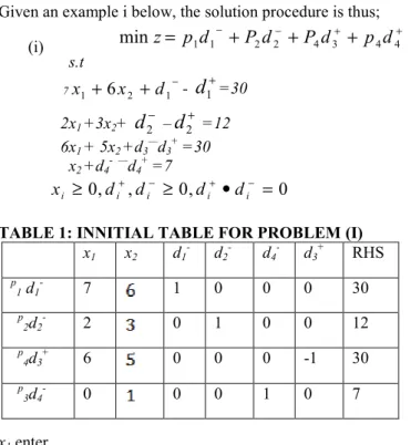
Given an example i below, the solution procedure is thus; (i) + + − −
+
+
+
=
1 1 2 2 4 3 4 4min
z
p
d
P
d
P
d
p
d
s.t 7x
1+
6
x
2+
d
1−- + 1d
=30 2x1 +3x2+ − 2d
–d
2+ =12 6x1 + 5x2 +d3—d3+ =30 x2 +d4- —d4+ =7≥
0
,
,
≥
0
,
•
=
0
− + − + i i i i id
d
d
d
x
TABLE 1: INNITIAL TABLE FOR PROBLEM (I)
x1 enter d1
-
leaves
The above table (1) is the initial table of problem (i). Column one represents the variables in z with priorities assigned to each of them which forms the bases. Columns two and three represent the coefficients of the decision
x1 x2 d1- d2- d4- d3+ RHS p 1 d1- 7 1 0 0 0 30 p 2d2- 2 0 1 0 0 12 p 4d3+ 6 0 0 0 -1 30 p 3d4 - 0 0 0 1 0 7
variables (aij) in the goal constraints equation. Columns four to seven represent coefficient of deviational
variables (citv) in the goal constraint equations that appeared in the achievement function. Column eight is the
right hand side values of the constraints equations. Applying the algorithm, step 1. set k=1.
Step 2.
∃
b
i = 0 for i=1,2,. . ., 4, {So solution feasible.}Step 3. ∃
g
1j>0 for some j. {So solution not optimal}. Since there is positive coefficient in the priority row, then the solution is not optimal.Step4. Max {gi}=max{7, 6, 1, 0,0,0,}=7 at g11 i.e. x1=7 enters the bases since
it is the highest in the row.
step 5 Min
{
:
10
}
1 i>
g bg
i i = min{30/7, 6, 5,}= 30/7 at[ ]
11 1 g b . So d1- leaves thebases. i.e the minimum ratio of the right hand side to the entrying column. Step6. Perform the normal gauss Jordan’s simplex operation to update the new
Tableau (see Tableau 2) and check if
p
1is still in the basis (CB) to test foroptimality.
TABLE 2: 1st ITERATION FOR PROBLEM(i)
x2 enter d2
leaves
Table (2), shows that
p
1 is satisfied since it is no longer in the bases. Step7. Set k=2. Since 2 < L=4, go to step 3.Step3. ∃
g
2j>0 for some j. i.e 2nd
priority row. {So solution not optimal} Step4.
max{
g
2j}
=max {0,9/7,-2/7,1,0,0}=9/7 at g22. So, x2enters the basis.Step5. Min
:
20
2 i>
g bg
i i =min {5, 8/3,7}= 8/3 at 22 2 g b. d2- leave since it has the smallest minimum
ratio.
Step 6. Perform the same operation to update the new tableau Table 3 and check if
p
2is still in the basis (CB) to test for optimality.Table 3: 2ND ITERATION FOR PROBLEM (i)
d2+ enter x1 Leaves
Table (3), shows that
p
2 is satisfied since it is no longer in the bases. Step7. Set k=3. Since 3 < L=4, go to step 3.Step3. ∃
g
4j >0 for some j. i.e 3th
priority row. {So solution not optimal} Step4.
{max
g
4j}
=max {0,0, 2/9,-7/9,1,0}= 97 −
at g44. So, d2+ enters the basis.
Step5. Min 4 i i g b :
g
i4>
0
=min {3, 39/7}= 3 at 14 1 g b. So x1 leave since it has the smallest minimum
ratio. x1 x2 d1 - d2 -d4 - d3 + RHS x1 1 6/7 1/7 0 0 0 30/7 p 2d2- 0 9/7 -2/7 1 0 0 24/7 p 4d3- 0 -1/7 -6/7 0 0 -1 30/7 p 3d4- 0 1 0 0 1 0 7 x1 x2 d1- d2- d4- d3+ RHS x1 1 0 1/3 -2/3 0 0 2 x2 0 1 -2/9 7/9 0 0 8/3 p 4d3+ 0 0 -8/9 1/9 0 -1 14/3 p 3d4- 0 0 2/9 -7/9 1 0 13/3
Step 6. Perform the same operation to update the new tableau Table 4 and check if
p
3is still in the basis (CB) to test for optimality.Table 4: 3RD ITERATION FOR PROBLEM (i)
d1+ enter d3+ leaves
Table (4), shows that
p
3 is not satisfied since it is still in the bases. Step3. ∃g
4j >0 for some j. i.e 3th
priority row. {So solution not optimal} Step4.
{max
g
4j}
=max {-7/6,0, 1/6, 0, 1,0, 0}=1/6 at g43. But , d1- cannot re-enterfor lower priority to leave the basis. Therefore p3 cannot be satisfied further,
so go to step 7.
Step7. Set k=4 and go to step 3. Step3. ∃
g
3j >0 for some j. i.e 4th
priority row. {So solution not optimal}
Step4.
{max
g
3j}
=max {1/6,0, -5/6,0,0, 0,-1}=5/6 at atg
33 . So, d1+ enters the basis.Step5. Min 3 i i g b :
:
g
i3>
0
=min {6}= 6 at 33 3 g b . So d3+ leave..Step 6. Perform the same operation to update the new tableau Table 5 and check if
p
4is still in the basis (CB) to test for optimality.Table 5: 4TH ITERATION FOR PROBLEM(i)
d3+ reenter d4- leaves
Table (5), shows that
p
4 is satisfied since it has left the bases. But p3 can be improved.Step3. ∃
g
4j >0 for some j. i.e 3th
priority row. {So solution not optimal} Step4.
{max
g
4j}
=max {-6/5,0, 0, 0, 1, 0, 0,1/5}=1/5 at g48. so , d3+ re-enterfor higher priority to leave the basis. Step5. Ming8
:
i8>
0
bg
i i =min {5}=5 at g48. So d4 leave.Step 6. Perform the same operation to update the new tableau Table 6 and check if
p
4is still in the basis (CB) to test for optimality.Table 6: Final iteration
Z=5 x1 x2 d1- d2- d4- d2+ d3+ RHS d2+ 3/2 0 1/2 -1 0 1 0 3 x2 7/6 1 1/6 0 0 0 0 5 p 4d3+ 1/6 0 -5/6 0 0 0 -1 5 p 3d4- -7/6 0 1/6 0 1 0 0 2 x1 x2 d1- d2- d4- d1+ d2+ d3+ RHS d2+ 8/5 0 0 -1 0 0 1 -3/2 6 x2 6/5 1 0 0 0 0 0 -1/5 6 d1+ 1/5 0 -1 0 0 1 0 -6/5 6 d4 - -6/5 0 0 0 1 0 0 1/5 1 x1 x2 d1- d2- d4- d1+ d2+ d3+ RHS d2+ 37 0 0 -1 0 1 0 27/2 x2 0 1 0 0 1 0 0 0 7 d1+ -7 0 -1 0 6 1 0 0 12 d3+ -6 0 0 0 5 0 0 1 5
The above is optimum since they cannot be achieved further.
5.RESULT
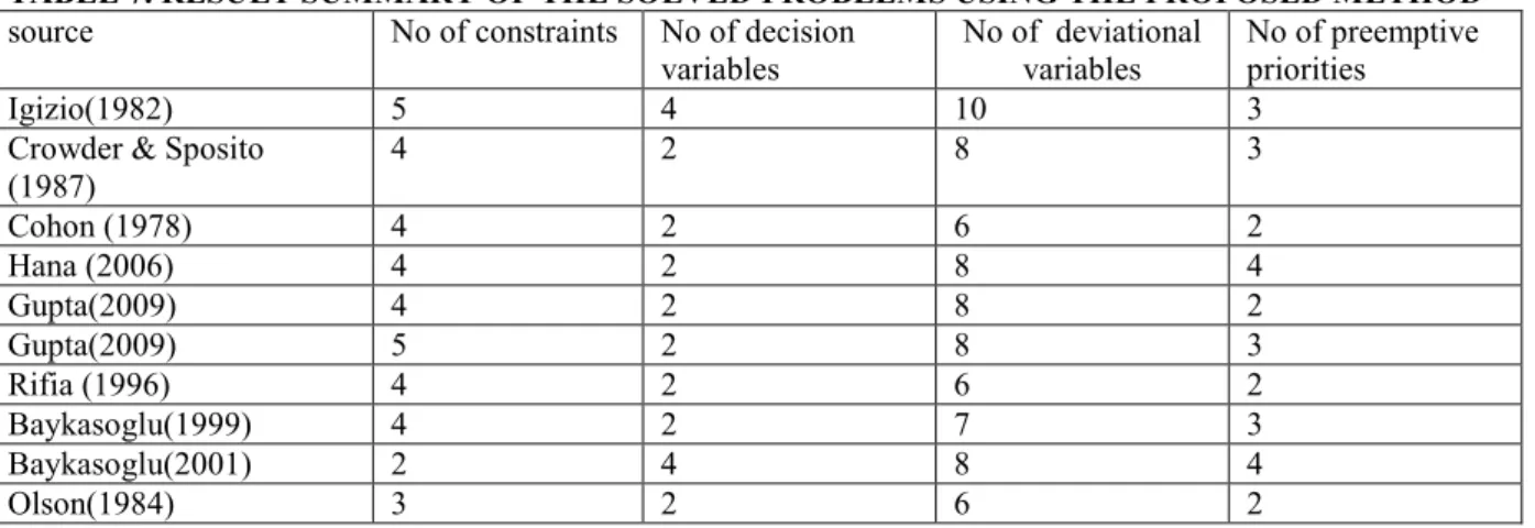
Problems from standard published papers of various sizes and complexities were solved to test the efficiency of the new lexicographic algorithm. The models varied widely in the number of constraints, decision variables, deviational variables and pre-emptive priority levels as shown in the table below.
TABLE 7. RESULT SUMMARY OF THE SOLVED PROBLEMS USING THE PROPOSED METHOD
source No of constraints No of decision variables No of deviational variables No of preemptive priorities Igizio(1982) 5 4 10 3
Crowder & Sposito (1987) 4 2 8 3 Cohon (1978) 4 2 6 2 Hana (2006) 4 2 8 4 Gupta(2009) 4 2 8 2 Gupta(2009) 5 2 8 3 Rifia (1996) 4 2 6 2 Baykasoglu(1999) 4 2 7 3 Baykasoglu(2001) 2 4 8 4 Olson(1984) 3 2 6 2 6 CONCLUSION
The proposed method is an efficient method of solving lexicographic Goal programming. The new method is used in solving various lexicographic linear Goal programming problems of different variables sizes, goals, constraints and deviational variables. The proposed method is an efficient method and its formulation represents a better model than the existing ones.
REFERENCES
[1] C.L Hwang, A. S. M. Masud, S.R Paidy, and K. Yoon, Mathematical programming with multiple objectives: a tutorial. Computers & Operations Research. (1980). 7, 5-31.
[2] Evans G.W An Overview of technique for solving multiobjective mathematical programs. Maence 30,(11) (1984) 1268-1282.
[3] Aouni,B. & O. Kettani, Goal programming model: A glorious history and promising future. European Journal Of operation of operational research 133, (2001), 225-231
[4] Sunnar, M and Kahrama, R A Comparative Study of Multiobjective Optimization Methods in Structural Design. Turk J Engin Environ Sci 25, (2001), 69 -86.
[5] Tamiz M, &D. F Jones (2010): Practical Goal Programming. International Series in Operations
Research & Management Science. Springer New York http://www.springer.com/series/6161.
[6] Schniederjans, M. J. & N. K. Kwak An alternative solution method for goal programming problems: a tutorial. Journal of Operational Research Society.33, (1982) 247-252.
[7] Hwang, C. &, K. Yoon (1981). Multiple Attribute Decision Making Methods and Applications - A State of the Art Survey. Springer- Verlag.
[8] IJiri, Y. (1965). Management Goals and Accounting for Control. Rand-McNally: Chicago. [9] Lee, S. M. (1972). Goal Programming for Decision Analysis. Auer Bach, Philadelphia.
[10] Ignizio J. P.(1976). Goal Programming and Extensions. D. C. Heath, Lexington, Massachusetts. [11] Ignizio, J.P A Note on Computational Methods in Lexicographic Linear Goal Programming. Opl Res. Soc. Vol. 34, No. 6, pp. 539-542, 1983 0160-5682.
[14] Ignizio J. P An algorithm for solving the linear goal-programming problem by Solving its dual. Journal of operational Research Society, 36, (1985) 507-5 15.
[15] Olson, D. L. Revised simplex method of solving linear goal programming problem. Journal of the Operational Research Society Vol. 35, No. 4(1984) pp 347-354.
[16] Orumie,U.C &D.W Ebong An Alternative method of solving Goal programming problems. Nigerian Journal of Operations Research vlo2,No 1, (2011) pg 68-90.