HAL Id: hal-02321656
https://hal.archives-ouvertes.fr/hal-02321656
Submitted on 15 Jan 2020
HAL
is a multi-disciplinary open access
archive for the deposit and dissemination of
sci-entific research documents, whether they are
pub-lished or not. The documents may come from
teaching and research institutions in France or
abroad, or from public or private research centers.
L’archive ouverte pluridisciplinaire
HAL, est
destinée au dépôt et à la diffusion de documents
scientifiques de niveau recherche, publiés ou non,
émanant des établissements d’enseignement et de
recherche français ou étrangers, des laboratoires
publics ou privés.
Distributed under a Creative Commons
Attribution| 4.0 International License
A review on dimensionality reduction for multi-label
classification
Wissam Sibblini, Pascale Kuntz, Franck Meyer
To cite this version:
Wissam Sibblini, Pascale Kuntz, Franck Meyer. A review on dimensionality reduction for multi-label
classification. IEEE Transactions on Knowledge and Data Engineering, Institute of Electrical and
Electronics Engineers, 2019, �10.1109/TKDE.2019.2940014�. �hal-02321656�
A Review on Dimensionality Reduction for
Multi-label Classification
Wissam Siblini, Pascale Kuntz and Frank Meyer
Abstract—Multi-label classification has gained in importance in the last decade and it is today confronted to the current needs to process massive raw data from heterogeneous sources. Therefore, dimensionality reduction, which aims at reducing the number of features, labels, or both, knows a renewed interest to enhance the scaling properties of the classifiers and their predictive
performances. In this paper we review more than fifty papers presenting dimensionality reduction approaches for multi-label classification and we propose an analysis in three steps : (i) a typology of the methods describing the main components of their strategies, the problem they tackle and the way they solve it (ii) a unified formalization of the problems to help to distinguish the similarities and differences between the approaches, and (iii) a meta-analysis of the published experimental results inspired by the consensus theory to identify the most efficient algorithms.
Index Terms—Dimensionality reduction, multi-label classification, meta-analysis.
1
I
NTRODUCTIONT
HEmost popular classification paradigms are the singlelabel classification and the multi-class classification. For the first one, the objective is to decide, for each instance described by its features, whether it is associated to a given label or not. The second one is a generalization and it aims at associating each instance to one label among several. How-ever, in many real-world applications (e.g. sound analysis [1] [2], computer vision [3] [4], text analysis [5] [6], biology and health [7] [8], recommender systems [9] [10]), items are intrinsically describable with multiple labels. For instance, in a Video on Demand catalog, a movie is described by a set
of complementary labels (e.g. Funny,Masterpiece, Based on
novel,Futuristic) which are used by a recommender system to provide users with movies that are relevant to their preferences. Consequently, multi-label classification, which associates each instance to multiple labels, has received a great attention in recent years. From the pioneering works of Boutell and al. [11], Zhang and al. [12] and Tsoumakas and al. [13], several reviews have been published [13] [14] [15] [16] [17] [18]. They group the algorithms in three main families : (i) the problem transformation methods which transform the multi-label problem into one or several single-label classification or regression problems, (ii) the algorithm adaptation methods which adapt existing algorithms to learn from multi-label data and (iii) the ensemble methods which deduce multi-label predictions from a collection of learners.
This effervescence in research has allowed a significant improvement of the result quality for benchmarks routinely used in the literature. But it has also coincided with the explosion of data dimensionality. In particular, today, the ex-pansion of online labeling services generates a production of massive raw data of varying quality. This scaling evolution has recently led to the emergence of the so-called eXtreme Multi-label Learning community which considers problems in which the number of labels is extremely large (in the order
of106
and more) [19] [20] [21]. This increasing complexity entails a renewed interest for the dimensionality reduction
approaches which aim at reducing the number of features, labels, or both in order to improve the scaling properties of the classifiers and their predictive performances.
Dimensionality reduction has a long history in data science [22] [23] associated to different motivations such as, in particular, data visualization and interpretation [24], data compression [25] and data denoising [26]. In short, applying dimensionality reduction on raw data offers a synthetized representation which allows highlighting links and structures hidden in the mass and guiding learning algorithms [27] [28]. As a promising lever for dealing with large and noisy data, dimensionality reduction in multi-label classification has been the subject of a large number of publications over the last decade, resulting in various developments of methods. However, to the best of our knowledge, only one state-of-the-art was already published five years ago [29] and it neither explores the wide range of existing approaches nor provides a global framework to compare them.
For the study presented in this paper, we have gathered more than fifty papers to provide a macroscopic view of the dimensionality reduction strategies developed in multi-label classification and to help users select the most efficient ones. Let us note that we do not consider the variable selection methods (see [30] for a recent review) which are efficient to change the relative importance of variables but which are not designed to extract semantic links between variables as pointed out by several authors [31] [32]. Here we go beyond a classical state-of-the-art often based on an organized list of the existing works by structuring our anal-ysis of the literature along three complementary objectives : (1) a typology of the different approaches, (2) a unified formalization of the problems, and (3) a meta-analysis of the published experimental results. The typology is built from the main components which determine the nature of the problem and the way to solve it: (i) the choice of the reduced space (feature space, label space or both), (ii) the indepen-dence/dependence between the dimensionality reduction
objective and the classification objective, (iii) the character-istics of the transformations which reduce the initial spaces, and (iv) the regularization functions and set of constraints which improve the problem solving process. To help to distinguish the similarities and differences between the approaches with more precision, we introduce two generic formulations which scan the large majority of the problems encountered in the literature. We complete this thorough review of the problem ingredients by a meta-analysis of the experimental comparisons carried out in the papers inspired by the consensus theory [33] [34]. For each selected evaluation measure, the published pairwise comparisons
(algorithmAiis better than algorithmAjat a statistical
sig-nificance levelα) are represented by a multigraph where the
vertices are the algorithms and the directed edges represent the domination relationships extracted from the published experimental results. The analysis of the multigraphs allows to identify communities which are families of algorithms that have been mostly examined separately in the littera-ture. Moreover, in each community, the approaches which outperform the others are highlighted.
2
T
YPOLOGY OFM
ULTI-L
ABELD
IMENSIONALITYR
EDUCTIONM
ETHODSThroughout the paper we consider a dataset with N
in-stances described by a set ofnx features and labeled by a
set ofnylabels. We denote byX(resp.Y) theN×nx(resp.
N×ny) matrix describing the features (resp. the labels). As
usually done in the literature,X (resp.Y) also refers to the
feature (resp. label) space when there is no ambiguity. The objective of the multi-label classification is to predict the
right label vectory ∈ Rny for any feature vector x ∈ Rnx.
During a training phase, given the feature matrix X, a
classifier is adjusted to fit its prediction to the label matrix Y.
The vast majority of multi-label classification approaches based on dimensionality reduction follows a two-step pro-cess : (1) reduction of X or Y or both, (2) prediction of the labels from the reduced spaces with a classifier. The dimen-sionality reduction is very often applied as an independent data pre-processing before prediction, but recent research stimulates exploration of the coupling between reduction and classification [35]. Whatever the strategy, the impact
of the reduction on the classifier performances is in fine
evaluated by the quality of the label prediction for which numerous measures have been proposed in the literature (e.g. Hamming Loss, F1) [14] [17]. Consequently, three in-gredients are considered in the dimensionality reduction
problem: the objective function fd for the dimensionality
reduction which is independent from or dependent on the
classifier, the objective functionfcassociated to the classifier
and the final prediction quality measure mq. Finally, the
choice of the reduced space closely determines the nature of the problem and the way to solve it.
Let us denote the reduction of X (resp. Y) by theN×kx
(resp.N×ky) matrixX′(resp.Y′) wherek
x(resp.ky) is the
dimension of the reduced spaceX′ (resp. Y′). In practice,
the values ofkxandkyare often fixed a priori (100and500
are commonly used values [36] [37]) but different classical strategies can be applied to guide their choice in particular
when the reduction method performs an
eigendecomposi-tion (e.g.kxand/orkyare the number of eigenvalues above
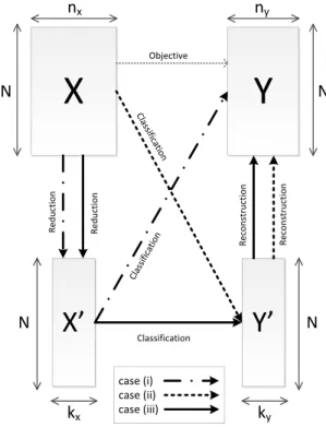
a fixed threshold, or necessary to preserve a percentage of the total sum of eigenvalues). There are three different ways to tackle the dimensionality reduction problem for the multi-label classification (figure 1): (i) reduce the feature
space X into X′ and predict the label matrix Y from the
reduced feature matrixX′, (ii) reduce the label spaceY into
Y′ and predict the reduced label matrixY′from the feature
matrixX, (iii) reduce both the label and the feature spaces
intoX′andY′and predict the reduced label matrixY′from
the reduced feature matrixX′.
X
Y
X’
ClassificationY’
Re ducti on Re co nstructi on Objective Classifi cation Classifi cationN
n
xn
yk
yk
xN
N
N
case (i) case (ii) case (iii) Re ducti on Re co nstructi onFig. 1. Overview of the dimensionality reduction strategies in the multi-label classification process.
For each of these cases, the dimensionality reduction problem can be set as an optimization problem:
optimize U,V fd(U, V, X, Y) +r(U, V) subject to c(U, V, X, Y) (1) where :
• U andV are either the parameters of a
transforma-tion functransforma-tion onXandY (e.g. projection matricesPx
andPy in the case of a linear transformation) or the
reduced matricesX′andY′. When a method reduces
one space only (eitherXorY) the problem is defined
with one parameter (UorV).
• fd is the reduction objective function which is
inde-pendent from or deinde-pendent on the classifier.
• r is a regularization function often associated to a
norm (L1,L2,L12) on the parameter space which is
introduced to limit the overfitting phenomena and to simplify the model.
• c is a constraint set on the search space. Some
ap-proaches do not introduce constraints but most of them try to reduce the degree of freedom of the problem to make its resolution easier.
In the following we detail the different ingredients of the problem (1). We first present the most popular objective
functions fd which are independent of the classifiers and
we specify their definitions according to the spaces targeted with the dimensionality reduction. Then, we discuss the different cases where the dimensionality reduction objective is coupled with the classification objective. For each case, only one example from the literature is given for illustration and we refer to Table 2 for a detailed state-of-the-art. In addition, Tables 1a and 1b synthetize the strategy of each of the reviewed methods. We finish with a synthetic pre-sentation of the regularization functions and the additional constraints applied by multi-label dimensionality reduction methods.
2.1 Classifier-Independent Objective Functions
We here present the dimensionality reduction methods with an objective function independent of the classifier. They are
grouped according to the space they reduce (X,Y, bothX
andY).
2.1.1 Feature Space Reduction (X)
The ”feature space reduction methods” turn the initial large
feature spaceXinto a reduced spaceX′
with the goal of ex-tracting the essential information of the data. As features are partially noisy, redundant and/or irrelevant, some works also aspire to fix the original defects [38]. The objective
functionfdis either independent from or dependent on the
information carried by the labels.
Most of the label-independent methods have been ini-tially developed for other learning paradigms but quite a few of them have also been frequently applied in multi-label learning. Their objectives can be organized into three families depending on the considered information for the
reduction1:
1) Objective FI1: maximize the conservation of the fea-ture covariance/co-occurrences (e.g. Principal Com-ponent Analysis (PCA) [39]);
2) Objective FI2: minimize the reconstruction error
for-mulated by a distance between X and X′
(e.g. Autoencoders (AE) [40]);
3) Objective FI3: maximize the conservation of
dis-tances between items described by X and by X′
(e.g. Locality Preserving Projection (LPP) [41]). The conservation is either global if all pairwise distances are equally maintained or local if, for example, each item only preserves its distances with its nearest neighbors.
Let us remark that these objectives may be closely linked together; for instance, PCA, classified in FI1, also implicitly minimizes the quadratic reconstruction error between a
1. Each objective is encoded to be identified in Table 2. For instance, FI1 refers to the1st objective of the label-IndependentFeature reduction methods.
projection of X′
and X (FI2). In addition, besides these
approaches, random projections (Objective R) have been explored [42] [43].
The label-dependent objectives aim at guiding the reduc-tion with label informareduc-tion [44] [45]. This helps to strengthen
the link between the extracted reduced feature spaceX′
and
the label spaceY. They cover three main strategies:
1) Objective FD1: maximize the X-Y link via a stan-dard criterion (covariance, Hilbert-Schmidt Inde-pendence) (e.g. Multi-label Dimensionality Reduc-tion via Dependence MaximizaReduc-tion (MDDM) [35]) ;
2) Objective FD2: preserve the isometry between the
instances described in the initial label space Y and
the instances described in the reduced feature space
X′
(e.g. Hypergraph Spectral Learning (HSL) [46]) 3) Objective FD3: maximize the link between the
fea-ture and the label space by learning a subspaceX′
that can be used to reconstruct bothX andY (e.g.
Multi-label Latent Semantic Indexing (MLSI) [47]). In addition, several hybrid approaches optimize a
pa-rameterized trade-off (e.g θ1 objective FD1 + θ2 objective
FD2) between the above objectives (e.g. Maximizing fea-ture Variance and feafea-ture-label Dependence simultaneously (MVMD) [48]).
2.1.2 Label Space Reduction (Y)
As some labels are correlated, it seems intuitive to take these correlations into account to improve both quality and scalability of the classification [17]. This can be achieved by learning a dimensionality-reduced label space. One of the first label space reduction for multi-label classification was based on compressed sensing (CS) [25]. The transformation made by CS is a random projection without training (Ob-jective R). However in the prediction phase, CS solves an optimization problem for each instance to reconstruct the la-bel vector from a reduced one. Since then, various strategies have been proposed. Dually to the feature space reduction above, they are either independent from or dependent on the information carried by the features. And, the feature-independent objectives can be organized into three families similar to the label-independent feature space reduction:
1) Objective LI1: maximize the conservation of the label covariance (e.g. Principal Label Space Transforma-tion (PLST) [49] which is the equivalent of PCA applied to the label space);
2) Objective LI2: minimize the reconstruction error
for-mulated by a distance betweenY andY′
(e.g. Multi-label prediction via compressed sensing (CS) [25]). 3) Objective LI3: maximize the conservation of
dis-tances between items described byY and byY′
(e.g. Cost-sensitive Label Embedding with Multidimen-sional Scaling (CLEMS) [50])
Let us note that, similarly to PCA, PLST also implicitly minimizes the quadratic reconstruction error (LI2).
There are also feature-dependent objectives. Indeed, when considering dimensionality reduction for classifica-tion, reducing the labels while strengthening the links with
the features can be useful. Conditional Principal Label Space Transformation (CLPST) [51] is one of the first methods to reduce the labels with an objective dependent on the features and it has opened the way to many other feature-dependent label space reduction approaches. They
maxi-mize the correlations between X and Y′
to improve the predictability of one matrix from the other (Objective LD).
In addition, several hybrid approaches solve a
parametrized trade-off between minimizing the
reconstruc-tion error betweenY andY′
and maximizing the prediction
of the feature matrix X from the reduced label matrix Y′
(e.g. Dependence Maximization based Label space dimen-sionality Reduction (DMLR) [52]).
Note that when the label space is reduced and the
classification model is trained on Y′
, the latter predicts
reduced label vectorsy′
and it is necessary to reconstruct the
original label vectors yfrom it. Three cases are commonly
encountered in practice (the main associated methods are indicated in parentheses):
1) A reconstruction model Ψinv : y′ 7→ y is trained
during the reduction phase or after [53]. It allows to
reconstructyfromy′
in the test phase. When the
re-duction is based on an orthogonal projectionPy, the
reconstruction is often computed by the transpose
projection (y′ 7→ y= PT yy ′ ). (PLST, MOPLMS, ML-CSSP, CPLST, BML-CS, FaIE, Rembrandt, DMLR, TRANS, LEML, Bi-Dir, BMLPL, GIMC, C2AE, WS-ABIE, COMB)
2) If the dimensionality reduction method explicitely
provides a reduction function Ψ : y 7→ y′
, then,
given a reduced label vector y′
, the original label
vector ycan be recovered by solving the following
structured output learning [54] problem: min
y l(y ′
,Ψ(y)) (2)
where l is a loss function. The optimization is
of-ten performed with matching pursuit [55] or basis pursuit [56]. (CS, MLC-BMaD, MSE)
3) The nearest neighbors ofy′
are computed in the
re-duced training set andyis deduced from the
aggre-gation of their original label vectors [37]. (CLEMS, SSI, SLEEC)
2.1.3 Both Feature Space and Label Space Reduction When both spaces are reduced, the reduction of each space depends on the other and two main strategies have been investigated:
• Objective LFD1: seek the principal directions in both
label space and feature space which maximise the linear correlations with each other. Originally de-veloped with the popular method CCA (Canoni-cal Correlation Analysis) [23] this approach has led to dozens of extensions in multi-label classification (e.g. an extension with a least square resolution LS-CCA [29], an extension with a sketching technique [57], an output-code extension [58]). Moreover, some methods have extended CCA by combining it with other approaches (e.g. The Two-Stage Dual Space Reduction Framework (2SDSR) [59]).
• Objective LFD2: minimize a distance function
be-tweenX′
andY′
(e.g. Supervised Semantic Indexing SSI [60]).
In addition, note that there is a special case (Independent Dual Space Reduction (IDSR) [61], [62]) where the label and feature space reductions are independently operated (objective LFI): a label-independent feature space reduction
is applied on X and a feature-independent label space
reduction is applied onY.
2.2 Coupling Dimensionality Reduction with the Clas-sifier Objective
As previously pointed out, a large majority of the reduction approaches are applied as a data pre-processing indepen-dent of the classification stage. But this procedure can turn out to be lacking in flexibility in some cases: its perfor-mances may be high for some problems and degrade some others. Indeed, it has been observed on many benchmarks that the impact of a reduction method on the classification performances varies with the classifier and the datasets [48]. To overcome this limitation, some works have started in-vestigating the coupling between dimensionality reduction and classification. At first glance, this approach consists in setting the coupling as a multi-objective optimization problem which tries to optimize both the reduction and
the classifier objectives (resp. fd and fc) simultaneously.
This multi-objective/multi-parameter problem is difficult to
solve [63] [64] [65] and, in practice, fd and fc are
alterna-tively or jointly maximized via a linear combination (Ob-jective C1 - e.g. Simultaneous Large-margin and Subspace Learning Approach (TRANS) [66]). But, when we get down to the details, the coupling can also be set up in two other scenarios:
1) Objective C2: the dimensionality reduction is inte-grated within the classification model by replacing
X and Y by X′
and Y′
in fc and the objective
is consequently the maximization of fc (e.g Linear
Dimensionality Reduction for Multi-label Classifi-cation (MLSVM) [67]).
2) Objective C3: the dimensionality reduction objective
fd is implicitly designed to optimize the classifier.
This happens when the classifier is k-NN. For
in-stance, Supervised Orthonormal Locality
Preserv-ing Projection (SOLPP) [68] learns a projection Px
on the feature space X that reduces the distance
between instances which share numerous labels.
This implicitly optimizes k-NN. Similar strategies
are employed in other methods (e.g. Hypergraph Spectral Learning (HSL) [46]).
2.3 Explicit and Implicit Transformations
When the algorithm reduces the data via a transformation function, the reduction is explicit and it allows to compute the transformation of any instance on line. Otherwise, the transformation is implicit: it directly provides the reduced matrix but not the transformation function.
# Method Description
1 Principal Component Analysis Eigendecomposition of the feature covariance matrix to derive orthogonal directions of
(PCA) maximal variance (principal components).
2 Locality Preserving Projection Spectral decomposition of the instance adjacency graph to compute a reduced feature
(LPP) space that maximally preserves it.
3 Constrained Non-negative Matrix Constrained non negative matrix factorization onX. The first factor is considered as the
Factorization (CNMF) reduced feature spaceX′.
4 Random Principal Component Analysis Randomized algebra technique (much faster than PCA whennxis large) to approximate
(RPCA) the principal components ofX.
5 Auto-Encoder Non linear reduction (projection + activation) and decoding to efficiently reduce and
(AE) reconstruct the original feature space.
6 Model-Shared Subspace Boosting Multiple random reductions of the feature space to create and combine a set of weak
(MSSBoost) classifiers.
7 Orthonormal Locality Preserving Extension of LPP with an orthonormality constraint on the reduced feature space.
Projection (OLPP)
8 Orthonormal Neighborhood Preserving Orthonormal feature space projection which preserves each item location with respect to
Projection (ONPP) itslnearest neighbors.
9 Shared subspace for multi-Label Embedding resulting from a trade-off between the label space and the feature space
(M LLS) reconstructions.
10 Partial Least Square Construction of a dimensionality reducing projection that maximizes the correlations
(PLS) between the projected feature space and the label space.
11 Multi-label Latent Semantic Indexing Linear feature space projection to optimize both the reconstruction of the original feature
(MLSI) space and the correlations between the projected feature space and the label space.
12 Orthonormal Partial Least Square Extension of PLS with an orthonormality constraint on the reduced feature space.
(OPLS)
13 Hypergraph Spectral Learning Spectral decomposition of an hypergraph which links instances with many common
(HSL) labels to obtain a reduced feature space that favors locality between them.
14 Joint Dimensionality Reduction and Multi- Simultaneous learning of a feature space reducing projection and an SVM classifier
label Classification (MLSVM) applied on the obtained reduced space.
15 Multi-Label Dimensionality reduction via Linear projection of the feature space that produces a reduced space with a minimal
Dependence Maximization (MDDM) Hilbert Schmidt Independence with the label space.
16 Semi-Supervised Dimension Reduction for Construction of a feature space projection which reproduces the neighborhood of the
Multi-Label Classification (SSDR-MC) instances in the label space in the projected feature space.
17 Supervised Orthonormal Locality Preserving Spectral decomposition of a feature/label adjacency trade-off graph to obtain a reduced
Projection (SOLPP) feature space where neighbors have common features and labels.
18 Multi-label Linear Discriminant Analysis Proposition of a definition for multi-label interclass/intraclass variances and
(MLDA) computation of the linearly reduced feature space that maximizes their ratio.
19 Direct Multi-label Linear Discriminant Redefinition of MLDA’s interclass variance matrix to overcome a limit that MLDA has
Analysis (DMLDA) on the dimensionality of the reduced space.
20 Variable Pairwise Constraint projection Proposition of ”must/cannot link” constraints between instances (based on their labels)
for Multi-label Ensemble (VPCME) and computation of the feature space projection that maximally respects them.
21 Hypergraph Orthonormal Partial Least Trade-off between OPLS and HSL.
Square (HOPLS)
22 Shared Subspace Multi-Label Dim reduction Trade-off betweenM LLS and MDDM.
via Dependence Maximization (SSMDDM)
23 Maximizing feature Variance and feature- Trade-off between PCA and MDDM.
label Dependence simultaneously (MVMD)
24 Multi-label prediction via Compressed Reduction of the label space with a random projection and reconstruction of it with a
Sensing (CS) sparse signal identification technique.
25 Principal Label Space Transformation Dually to PCA, computation of the orthogonal directions of maximum variance
(PLST) (principal components) in the label space.
26 Bayesian Multi-Label Compressed Sensing Simultaneous learning, with EM, of probabilistic models for (i) labels reduction, (ii)
(BML-CS) reduced labels prediction and (iii) labels decoding.
27 Multi-Label Classification via Boolean Boolean Matrix Decomposition to construct the binary reduced label space that can
Matrix Decomposition (MLC-BMaD) optimally reconstruct the original label space.
TABLE 1a
# Method Description
28 Landmark Selection Method for Multiple Resolution of a strongly regularized label space encoding/decoding problem and
Output Prediction (MOPLMS) selection of the non-zero labels in the solution as the reduced label space.
29 Multi-Label Column Subset Selection Derivation of label weights from the spectrum of the label covariance matrix and label
Problem (ML-CSSP) sampling with the weighted probability to produce the reduced spaceY′.
30 Cost-sensitive Label Embedding via Multidimensional scaling of the label space to embed instances according to a chosen
Multidimensional Scaling (CLEMS) instance pairwise cost which reflects the similarity of their label vector.
31 Conditional Principal Label Space Combination of PLST and CCA to guide label space reduction with feature information.
Transformation (CPLST)
32 Multi-label Subspace Ensemble Dimensionality reduction of the label space to improve its linear correlations with the
(MSE) feature space.
33 Feature-aware Implicit label space Implicit reduction of the labels to maximize (i) their ability to reconstruct the original
Encoding (FaIE) labels and (ii) their correlation with the feature space.
34 Response EMBedding via RANDomized Eigenvalue decomposition of the feature-label covariance matrix with a sketching
Techniques (Rembrandt) technique to reduce the label space and improve its link with the feature space.
35 Dependence Maximization based Label Trade-off between PLST and MDDM.
space dimension Reduction (DMLR)
36 Multi-Label Adapatative Random Computation of the feature space projection with an RVNS heuristic that optimizes the
Projection (ML-ARP) performances of the multi-label classifier ML-kNN on the reduced feature space.
37 Independent Dual Space Reduction Independent application of PCA on the feature space and PLST on the label space.
(IDSR)
38 Canonical Correlation Analysis Computation of the principal directions in both label and feature spaces that
(CCA) maximizes their linear correlations with each other.
39 Supervised Semantic Indexing Reduction of the feature space and the label space to increase (resp. decrease) the
(SSI) similarity between relevant (resp. irrelevant) pairx′-y′of feature and label vectors.
40 Least-Square Canonical Correlation Approximate solution of CCA using an equivalent least square expression and an
Analysis (LS-CCA) efficient resolution.
41 Regularized Canonical Correlation Regularized version of CCA with an improved behavior when the label-feature
Analysis (rCCA) covariance matrix is close to singular.
42 Web Scale Annotation By Image Embedding Construction of feature and label embeddings such as the instances’ features average
(WSABIE) representation is similar to their labels’ representation.
43 Simultaneous Large-margin and Subspace Combination and simultaneous training of an unsupervised feature reduction method
Learning Approach (TRANS) and a large margin multi-label classifier.
44 Deep Canonical Correlation Analysis Application of CCA onf1(X)andf2(Y)wheref1andf2are two deep neural
(DCCA) networks. CCA and the networks are trained simultaneously.
45 Supervised Dual Space Reduction Family of methods that apply an existing dependent feature space reduction method
(2SDSR) onX(e.g MDDM) and an existing dependent label space reduction method onY.
46 Convex Co Embedding Projection of the label and feature spaces which optimize a similarity, for each instance,
(ILA) between the reduced feature vector and reduced label vector.
47 Low rank Empirical risk minimization Simultaneous training of a classifier and a linear feature space reduction with the low
for Multi-Label Learning (LEML) rank Empirical Risk Minimization problem.
48 Bi-Directionnal Representation Learning Simultaneous predictions of labels from features and features from labels with an
(Bi-Dir) intermediary dimensionality reduction based on a bi-directional neural network.
49 Bayesian Multi-label Learning via EM-based construction of a subset of reduced labels (called topics) that can (i)
Positive Labels (BMLPL) reconstruct all the labels (Poisson law) and (ii) be predicted from features (Gamma law).
50 Sparse Local Embedding for Extreme Clustering of the instances and construction of local embeddings, on each cluster, of the
Classification (SLEEC) feature space to obtain the same closest neighborhood as in the label space.
51 Multi-label classification with feature-aware Union of a reduced features space obtained with CCA and a reduced feature space
non-linear label space transformation (COMB) obtained with KCCA.
52 Robust Extreme Multi-label Learning Prediction of labels using both a linear model applied on a linearly reduced feature
(REML) space and a sparse linear model applied on the original feature space.
53 Goal Inductive Matrix Completion Multi-label matrix completion technique to reduce the instance features and labels.
(GIMC)
54 Canonical-Correlated Auto-Encoder Combination of a label space auto-encoder with CCA to reduce the features and the
(C2AE) labels and to decode the predicted reduced labels.
TABLE 1b
Family Dependancy Method Ref Year Constraint/ Objective Type of Scale Scale Coupl.
of method Regularization Code transformation w.r.t w.r.t classif
N nxny
PCA [39] 1901 Orth. Transfo. FI1 Explicit Lin Yes No No
LSI [69] 1990 Uncorr. Space FI2 Implicit Yes No No
LPP [41] 2004 Uncorr. Space FI3 Explicit Lin No No No
CNMF [70] 2006 Uncorr. Space FI1 Implicit Yes Yes No
RPCA [71] 2006 Orth. Transfo. FI1 Explicit Lin Yes Yes No
Label AE [40] 2006 FI2 Explicit Non Lin Yes No No
Independent MSSBoost [72] 2007 R Explicit Lin No No No
OLPP [73] 2007 Uncorr. Space FI3 Explicit Lin No No No
ONPP [73] 2007 Orth. Transfo. FI3 Explicit Lin No No No
Feature PLS [74] 1983 Orth. Transfo. FD1 Explicit Lin Yes No No
Space MLSI [47] 2005 Uncorr. Space FD3 Explicit Lin Yes No No
Reduction OPLS [75] 2006 Uncorr. Space FD1 Explicit Lin Yes No No
HSL [46] 2008 Uncorr. Space FD2/C3 Explicit Lin No No Yes
M LLS [76] 2008 Orth. Transfo. FD3 Explicit Lin Yes No No
MLSVM [67] 2009 Orth. Transfo. C2 Explicit Lin Yes No Yes
MDDM [35] 2010 Orth. Transfo. FD1 Explicit Lin Yes No No
Label SSDR-MC [77] 2010 Uncorr. Space FD2/C3 Implicit No No Yes
Dependent SOLPP [68] 2010 Orth. Transfo. FD2/C3 Explicit Lin No No Yes
MLDA [78] 2010 Orth. Transfo. FD1 Explicit Lin Yes No No
DMLDA [79] 2013 Orth. Transfo. FD1 Explicit Lin Yes No No
VPCME [80] 2013 Orth. Transfo. FD2/C3 Explicit Lin No No Yes
HOPLS [81] 2014 Uncorr. Space FD1/C3 Explicit Lin No No Yes
SSMDDM [82] 2015 Regularization FD1/FD3 Explicit Lin Yes Yes No
LM-kNN [83] 2015 C3 Explicit Lin Yes No Yes
MVMD [48] 2016 Orth. Transfo. FI1/FD1 Explicit Lin Yes No No
ML-ARP [84] 2017 C2 Explicit Lin No Yes Yes
CS [25] 2009 R Explicit Lin Yes Yes No
PLST [49] 2012 Orth. Transfo. LI1 Explicit Lin Yes No No
Feature MLC-BMaD [85] 2012 Binary Space LI2 Implicit No No No
Independent MOPLMS [86] 2012 Selection LI2 Explicit Yes Yes No
Label ML-CSSP [87] 2013 Selection LI1 Explicit Yes No No
Space CLEMS [50] 2016 LI3 Implicit No Yes No
Reduction
CPLST [51] 2012 Orth. Transfo. LD Explicit Lin Yes No No
MSE [88] 2012 C2 Implicit No No Yes
BML-CS [89] 2012 C1 Explicit Non Lin Yes No Yes
Feature FaIE [90] 2014 Uncorr. Space LD Implicit Yes No No
Dependent Rembrandt [91] 2015 LD Explicit Lin Yes Yes No
DMLR [52] 2015 Orth. Transfo. LD Explicit Lin Yes No No
Independent IDSR [61] 2013 Orth. Transfo. LFI Explicit Lin Yes No No
CCA [92] 1936 Uncorr. Space LFD1 Explicit Lin Yes No No
SSI [60] 2009 LFD2 Explicit Lin Yes Yes No
LS-CCA [92] 2011 Uncorr. Space LFD1 Explicit Lin Yes Yes No
rCCA [92] 2011 Uncorr. Space LFD1 Explicit Lin Yes No No
WSABIE [93] 2011 LFD2 Explicit Lin Yes Yes No
Feature TRANS [66] 2012 Regularization C1 Implicite Yes Yes Yes
Space DCCA [94] 2013 Uncorr. Space LFD1 Explicit Non Lin Yes Yes No
and Label 2SDSR [59] 2013 Several LFD1 Explicit Lin Yes No No
Space Dependent ILA [95] 2014 LFD2 Explicit Lin Yes Yes No
Reduction LEML [96] 2014 Regularization C2 Explicit Yes Yes Yes
Bi-Dir [53] 2014 C1 Both Yes Yes Yes
BMLPL [97] 2015 C1 Implicit Yes Yes Yes
SLEEC [37] 2015 Regularization C3 Both Yes Yes Yes
COMB [98] 2015 Uncorr. Space LFD1 Explicit Non Lin Yes No No
REML [99] 2016 Regularization C2 Both Yes Yes Yes
GIMC [100] 2016 Regularization LFD2 Explicit Non Lin Yes Yes No
C2AE [101] 2017 Orth. Transfo. C1 Explicit Lin Yes Yes Yes
TABLE 2
Dimensionality reduction methods, their typological family and criteria. We report ”yes” for scalability if the complexity is strictly under quadratic. The objective codes, which refer to the type of objective considered by the methods, are detailed in Section 2.
2.3.1 Explicit Transformations
The vast majority of the methods presented in that
re-view reduce dimensionality with projections (X′
= XPx
or Y′
= Y Py). They are consequently explicit and linear.
These linear transformations can be extended to a non linear transformation with the classical kernel trick and most of the linear methods have a kernel extension (e.g. kPCA [102] for PCA, kCCA [103] for CCA).
Additional non linear explicit approaches have been adapted for the multi-label case. They can be classified into three categories:
1) Locally Linear Embeddings [37] [104]: they
pro-duce a non linear transformation, depro-duced from a piecewise linear transformation, by partitioning the label and/or feature space and computing a specific linear transformation per region.
2) Representation learning with neural networks. The
target output depends on the network architecture. For the auto-encoders [40] the output is a recon-struction of the input layer. For the multi-label neural networks [105] [106] [107] the output is a prediction of Y (resp. X) and the input is X (resp. Y). More complex architectures, which combine auto-encoders and multi-layer perceptrons, have been re-cently investigated [101] [53]. For details, we refer to the complete review [27] on representation learning which includes several methods which have been adapted to multi-label classification [108].
3) Probabilistic process [109] [89] [97]. The
transforma-tion from the initial space (X orY) to the reduced
space (X′
or Y′
) is a combination of parameter-ized probability laws (often Normal, Dirichlet and Gamma distributions). In that case, the construction of the reduced space is achieved by inference.
2.3.2 Implicit Transformations
The implicit transformations directly provide the reduced space without explicitely computing the transformation op-erator (e.g. using Multi-Dimensional Scaling (MDS) [110] or Matrix Factorization [111]). They consequently have no reason to be linear. Direct learning of the reduced spaces
X′
orY′
offers more degree of freedom in the optimization problem but it is more frequently confronted to overfitting [112]. Moreover, it is not adapted to incremental processes: when a new item is added, the reduction must be fully relaunched. Nevertheless, the recent rise of extreme multi-label classification [19] [113] stimulates the development of implicit transformations [93] [37] [96] [90] [50]. They are adapted to the label space reduction because the online reduction of a label vector is not required. On the contrary, explicit transformations are more suitable for feature space reduction because the transformation of new feature vectors is necessary in the prediction phase.
2.4 Regularization and Constraints
Adding a regularization functionrto the objective function
fd or a set of constraints to the optimization problem (1)
aims at (i) reducing the degree of freedom of the problem, (ii) providing simpler transformations of the initial spaces
into the reduced ones by restricting the parameters, (iii) improving generalization and limiting overfitting and (iv) building more classification-friendly training sets. These objectives, which are common to many machine learning problems, are integrated in the optimization problem in a variety of ways:
• Sparse transformations. Some methods impose
spar-sity on the reduced space variables or on the reduc-tion funcreduc-tion parameters [37] [96]. Formally, sparsity
of a matrix is computed from itsL0-norm, but due to
its non-continuity and non differentiality the authors
usually resort to theL1-trick and relax theL0-norm
into aL1-norm [114]. In practice, this approach limits
overfitting, optimizes storage and speeds training and prediction up ;
• Limited search space. A major part of the algorithms
impose the minimization of the L2-norm of the
parameters. This benefits solutions with low-value parameters [53] [29].
• Sparse and small parameter sets. This is achieved
with an Elastic Net Regularization [115] which is a
linear combination ofL1andL2regularizations [37].
• Parameter clipping. This regularization restrains the
parameter definition domain to a fixed interval with thresholding techniques [116].
• Dropout regularization. Some neural network based
approaches regularize their parameters by using the dropout strategy [117] which selects a different ran-dom parameters subset at each training step. Moreover, constraints are also introduced to limit noise and variable correlations which are enemies of most clas-sifiers [118]. Two usual constraints aim at facilitating the classification task :
• Uncorrelated space. Classification is easier when
the correlations in the variable space are limited. Such a constraint can be express in the matrix form
X′TX′
= I (or Y′TY′
= I). Let us remark that
this constraint leads to a L2-norm regularization
(|X′
|2=tr(X′TX) =tr(I)).
• Orthonormal projection. This constraint is expressed
in the popular linear case byPTP =I.
Some authors have also proposed a trade-off PT((1−
µ)XTX+µI)P =I between these two constraints [48] [35].
3
T
WOG
ENERICP
ROBLEMF
ORMULATIONSThe previous section highlights the great variability of the different ways to adress the issue of dimensionality reduc-tion for multi-label classificareduc-tion. In the literature analysis, where each author resorts to his/her own formulation, this variability is an obstacle to a fine understanding of the similarities and differences between the approaches. To make the comparisons easier, we here propose two generic formulations of the general problem (1). The first one, closely linked to a generic scheme of resolution based on eigendecomposition, allows to express more than half of the problems. The second one is an extension which covers all cases. It is associated to a large variety of optimization pro-cesses (e.g. gradient descents, Newton method, Lagrangian techniques).
3.1 The Basic Framework
As we show in Table 3, a large number of problems can be written as follows : optimize U tr(UTA XYU) subject to UTBXYU=I (3) where :
1) AXY andBXY are matrices which are function ofX
andY.
2) according to the space that is reduced and the type
of transformation, the parameter U is one of the
following matrices :X′
,Y′
,Px, orPy.
3) the optimization goal is either a minimization or a
maximization objective.
Problems expressed by (3) can be solved with an eigen-decomposition. It is well-known that, using the Lagrangian
method [120], the problem (3) is equivalent to optimizeλin
the following generalized eigenvalue problem:
AXYu=λBXYu (4)
The solution U of (3) in the maximization (resp.
min-imization) case is therefore the matrix of the eigenvectors
associated to theklargest (resp. smallest) eigenvalues of (4).
In the frequent case where the matrix AXY is symmetric
positive, the eigenvectors ofAXY can also be retrieved by a
singular value decomposition [121] of the square rootRXY
ofAXY defined byRTXYRXY =AXY.
Despite its elegant solution, the eigenvalue
decomposi-tion (4) is computadecomposi-tionally complex: in the order ofn2
real-valued numbers for spatial complexity andn3
operations for temporal complexity [122]. For scaling, different approaches are used: fast eigendecomposition techniques (e.g. Jacobi [123] and QR [124]), approximation of the largest eigen-values (power iteration algorithm [125], Lanczos method [126]), matrix sketching [127] (e.g. in randomized PCA [71] or Rembrandt [91]). In addition, a reformulation of problem (3) in a least square form is also popular to resort to a numerical optimization method (e.g. least square version of CCA [92] or LDA [128]). Indeed, the initial least square
formminUminMkRXY−M UTk2F, whereRXY is the square
root ofAXY, is equivalent tomaxUtr(UTAXYU)with the
constraintUTU=I.
For illustration let us consider the classical formulation
of PCA maxPxtr(P
T
x(XTX)Px). Subject to PxTPx = I, it
can be reformulated into the mean squared reconstruction
error minimization problem minX′,PxkX −X′PxTk2F with
simple algebra. The strong constraintUTU=Iis sometimes
replaced with a simplerL2-regularization onU.
Let us note that a portion of the methods expressed with the basic framework (3) are based on graph spectral decom-positions [129] [130]. They follow a two-step procedure: (i) build a graph which links the instances with a proximity property (e.g distance on the label space) and (ii) embed the instances in a reduced space by preserving the graph neighborhood structure. The transformation is computed by an eigendecomposition of the normalized Laplacian of
the graph (AXY is the normalized Laplacian andBXY the
identity matrix).
3.2 Towards a General Framework
The equivalence between the basic framework (3) and a least square formulation highlights both its flexibility and its
lim-its.L1-regularizations [131], multi-label loss functions other
than mean square error [15] and many other items cannot be expressed as a matrix trace. An attempt at generalization has been proposed in [96]. The problem is set as a problem of minimization of the empiral risk (ERM) [132] which does not require a specific loss function nor any specified
regu-larization. Let us denote byh(x;Z) :x7→bythe classification
model of parameter Z, by l(y,yb) = l(y, h(x;Z)) the loss
function between the predicted label vectorbyand the true
label vectory, and byr(Z)the parameter regularization. The
low rank empirical risk minimization problem is expressed as follow: b Z=argmin Z N X i=1 ny X j=1 l(Yij, hj(xi;Z)) +λr(Z) subject to rank(Z)≤k (5)
Let us remark that this formulation differs from the
classical ERM problem: the added rank constraint on Z ∈
Rnx×ny entails a dimensionality reduction [133].
The formulation (5) covers a large part of the methods of the literature but to include the remaining uncovered cases, we propose a generic formulation of the objective function which is an additive combination of the essential ingredients encountered in the multi-label dimensionality reduction typology: J(X′ , Y′ , Zx, Zy, Zxy) =αxex(X ′ , X, Zx) +αyey(Y ′ , Y, Zy) +αxyexy(X′, X, Y, Y′, Zxy) +αpp(X ′ , Y′ ) +αrr(X ′ , Y′ , Zx, Zy, Zxy) (6) where:
• ex is a reconstruction error between X and its
re-duced versionX′
.
• ey is a reconstruction error between Y and its
re-duced versionY′
.
• exy is a joint error betweenX,Y,X′, andY′ which
can, for instance, express the classification error.
• ris a parameter regularization.
• Zx,Zy,Zxy are the parameters of the reduction and
the classification functions.
• pare additional properties imposed on both reduced
spaces.
The reconstruction errorex can be expressed with both
the encoding losslx1(reconstruction ofX′fromX) and the
decoding losslx2(reconstruction ofXfromX′):
αxex(X ′ , X, Zx) =αx1lx1(X ′ , fx1(X, Zx)) +αx2lx2(X, fx2(X ′ , Zx)) (7)
where thef functions are parametric models. This is also
Method U AXY Dependancy BXY Constraint Year Ref
PCA Px XTX No I Orth. Transfo. 1901 [39]
CCAx Px XTY(YTY)−1YTX Yes XTX Uncorr. Space 1936 [23] [92]
PLS Px XTY YTX Yes I Orth. Transfo. 1983 [74]
KPCA Px φ(X)Tφ(X) No I Orth. Transfo. 1997 [102]
LPP Px XTLX No XDXT Uncorr. Space 2004 [41]
MLSI Px XT((1−θ)XTX+θYTY)X Yes XTX Uncorr. Space 2005 [47]
OPLS Px XTY YTX Yes XTX Uncorr. Space 2006 [75]
RPCA Px XTX No I Orth. Transfo. 2006 [71]
KDA Px Sw−1Sb Yes I Orth. Transfo. 2007 [119]
OLPP Px XTLX No I Orth. Transfo. 2007 [73]
ONPP Px XT(I−W)(I−WT)X No I Orth. Transfo. 2007 [73]
HSL Px XLnXT No XTX Uncorr. Space 2008 [46]
MLLS Px S2−1S1 Yes I Orth. Transfo. 2008 [76]
MLSVM Px (XTX)†XTY YTX Yes I Orth. Transfo. 2009 [67]
MDDM Px XTHY YTHX Yes I Orth. Transfo. 2010 [35]
MLDA Px Sw−1Sb Yes I Orth. Transfo. 2010 [78]
SOLPP Px XT(I−W)(I−WT)X Yes I Orth. Transfo. 2010 [68]
SSDR-MC X′ XT(I−W)(I−W)TX Yes XTX Uncorr. Space 2010 [77]
rCCAx Px XTY(YTY)†YTX Yes XTX Uncorr. Space 2011 [92]
CPLST Py YTH(XXT)†HY Yes I Orth. Transfo. 2012 [51]
PLST Py YTY No I Orth. Transfo. 2012 [49]
DMLDA Px XTHY W−1YTHX Yes I Orth. Transfo. 2013 [79]
IDSRx Px XTX No I Orth. Transfo. 2013 [61]
IDSRy Py YTY No I Orth. Transfo. 2013 [61]
VPCME Px SC−θSM Yes I Orth. Transfo. 2013 [80]
FaIE Y′ Y YT+θX(XTX)−1XT Yes I Orth. Transfo. 2014 [90]
FaIE Linear Py YT(YTY +θX(XTX)−1XT)Y Yes YTY Uncorr. Space 2014 [90]
HOPLS Px XT(Y YT+θS)X Yes XTX Uncorr. Space 2014 [81]
DMLR Py YT(I+θHXXTH)Y Yes I Orth. Transfo. 2015 [52]
MVMD Px (1−θ)XTX+θXTHY YTHX Yes I Orth. Transfo. 2016 [48]
Notations:
M†: pseudo-inverse of a matrixM
L(resp.Ln): graph (resp. normalized) Laplacian
φ: kernel transformation
W,SC,SM,Sb,Sw,S: pairwise weight matrices
θ,α,β: trade-off parameters
H= (δij−N1)ijwhereδis the Kronecker delta
S1=I−αT−1andS2=T−1XTY YTXT−1whereT =N1X
TX+ (α+β)I
TABLE 3
Connection between dimensionality reduction methods and the basic objective framework(3)
In most cases, the regularization r can be additively
decomposed: αrr(X′, Y′, Zx, Zy, Zxy) =αr1r1(X ′ ) +αr2r2(Y ′ ) +αr3r3(Zx) +αr4r4(Zy) Y +αr5r5(Zxy) (8)
In (6), (7) and (8), theαconstants are weights that allow
trade-offs between the different components of the problem. All forms of (6) are tackled with customized numerical optimization methods [134] [135]. Considering the convex-ity, the smoothness, the order, the differentiability and the conditioning of the formulation, the problem is sometimes reformulated (convex relaxation [136], primal/dual conver-sion [137], preconditioning [138]) and the resolution is either performed with an adapted variant of the gradient descent [139] [140], a coordinate descent [141] or higher order al-gorithms such as Newton method [142] or Frank Wolfe’s algorithm [143]. Also, constrained problems are generally solved with a Lagrangian method [144], with one of its diverse extensions (e.g Augmented Lagrangian like ADMM [145] [37]) or with a projected gradient descent. The choice
of the couple formulation/resolution is essential: it affects the spatial and temporal complexities of the computations and the quality of the convergence towards the solution.
To be complete, let us point out that two families of dimensionality reduction methods explored for multi-label classification reach the limits of the generic formulation. The first one includes approaches based on mixture models [97] and solved with the suitable state-of-the-art EM algorithm and its variants [146] [147]. The second one includes the ensemble strategies (bagging [80] [88] and boosting strategy [72]) where multiple dimensionality reducing transforma-tions are trained on bootstraps and aggregated according to two main strategies. Each transformation produces its own reduced space and either the reduced spaces are aggregated into a global reduced space and the classifier is trained on it or a classifier is trained on each reduced space and the predictions of each classifier are aggregated.
4
M
ETA-
ANALYSISOur previous generic frameworks allow to explicitly iden-tify the different ingredients involved in the various
ap-proaches proposed in the literature and to help to under-stand their common points and differences. However in practice, a question persists: which are the most efficient ap-proaches? It is difficult to answer because only partial com-parisons are generally reported in the articles and to the best of our knowledge there exist no experimental studies which compare all the approaches presented in Table 2. Moreover, the computational implementations are very diverse and for some approaches the source codes or the parameter settings are even not available. Hence, a normalized comparison would entail a recoding of all the algorithms and a new battery of tests on a unified framework that remains to be defined in the research community. With the large set of al-gorithms to be considered, this would require a considerable time-consuming effort, and consequently the exploitation of the outcomes of the existing published research works appears as a more realistic alternative. The experimental protocols (datasets, classifiers, performance measures, etc...) varying from one publication to another, we here propose a new meta-analysis methodology.
Often defined as “the statistical analysis of a large col-lection of analysis results from individual studies for the purpose of integrating the findings” [148], the meta-analysis has known an increasing development from its pioneering works in the 30’s [149] [150]. One of its favored field is medicine where aggregation of the available pieces of infor-mation is required to make as rational as possible decisions. In computer science, this approach is still unusual as the great majority of researchers prefer to compare their own approaches with a restricted subset of existing ones on a set of benchmarks they habitually use but the first attempts (e.g. [151] [152] [153]) seem promising.
In this paper we aim at identifying the dimensionality reduction approaches used in multi-label classification for which several pieces of evidence show their domination over others: these approaches statistically obtain the best performances in the results published in the international conferences and journals with a review process. As it is well-known in multi-label classification that the performances can be evaluated with a wide range of measures we extract the relevant methods for each of the most frequently used and independent quality measures. In the following we first present a descriptive analysis of the observed occurrences and co-occurrences of the algorithms and of the measures, then we detail the process to extract the dominant ap-proaches, and finally we discuss the obtained results.
4.1 Methodology
From all the papers referenced in Table 2, we have retained a
corpusC of 27 papers –marked in bold type- which present
relevant and exploitable results for a meta-analysis. More precisely, we have first extracted the 32 papers that compare at least two methods, and then we have removed the 5 papers whose results are given on graphics only since they are difficult to exploit.
4.1.1 The Considered Algorithm Set
Let us denote byAthe set of the 42 algorithms that appear in
the selected papers of the corpusC. The published pairwise
comparisons can be described by a multigraph Gc: the
vertices represent the algorithms ofAand an edge is added
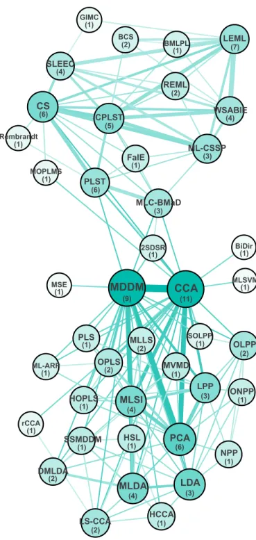
between two algorithms when they are compared in a paper. In the graph layout (Figure 2), the vertex diameter is propor-tional to the frequency of the associated algorithm and the edge set between a vertex pair is represented by a single edge whose width is proportional to the set cardinality.
2SDSR CCA MDDM MLC-BMaD PLST BCS BMLPL CPLST LEML WSABIE BiDir CS DMLDA HOPLS LPP LS-CCA ML-ARP MLDA MLLS MLSI MLSVM MOPLMS MVMD OLPP OPLS PCA PLS SOLPP rCCA FaIE ML-CSSP REML SLEEC GIMC HCCA HSL LDA SSMDDM NPP ONPP MSE Rembrandt (1) (2) (1) (7) (2) (4) (6) (5) (1) (1) (3) (1) (6) (3) (4) (1) (1) (1) (1) (2) (1) (1) (1) (1) (2) (2) (4) (1) (3) (6) (1) (1) (3) (4) (1) (2) (1) (2) (1) (1) (11) (9)
Fig. 2. Algorithm comparison multigraph for the 27 selected articles. The larger and the darker blue, the higher the weights of the edges and degrees of the vertices. The number of articles in which each algorithm appears is in parentheses.
The obtained layout is very different from the one of a complete graph which would be the ideal model, but far from reality, where each algorithm is compared to all others in many experiments. However, it highlights two
01Loss AUC Accuracy AveragePr ecision Coverage Err orRate F1 HammingLoss Macr oF1 Micr oF1 OneErr or
P@3 Precision RankingLoss Recall SubsetAccuracy Macr
oPr ecision Micr oPr ecision 01Loss 1 AUC 0 9 Accuracy 1 0 3 AveragePrecision 0 1 0 1 Coverage 0 1 0 1 1 ErrorRate 0 0 0 0 0 1 F1 1 0 3 0 0 0 7 HammingLoss 1 3 2 1 1 0 3 12 MacroF1 0 3 0 1 1 0 0 5 7 MicroF1 0 3 0 1 1 0 0 5 7 7 OneError 0 3 0 1 1 0 0 2 2 2 5 P@3 0 2 0 0 0 0 0 1 0 0 4 4 Precision 0 0 1 0 0 0 2 1 0 0 0 0 2 RankingLoss 0 1 0 1 1 0 0 1 1 1 1 0 0 1 Recall 0 0 1 0 0 0 2 1 0 0 0 0 2 0 2 SubsetAccuracy 0 0 1 0 0 0 1 1 0 0 0 0 1 0 1 1 MacroPrecision 0 0 0 0 0 0 0 0 1 1 0 0 0 0 0 0 1 MicroPrecision 0 0 0 0 0 0 0 0 1 1 0 0 0 0 0 0 1 1 TABLE 4
Matrix of the quality measure co-occurrences computed on the 27-article set. The occurrence of each measure is on the diagonal.
communities that correspond to two families of algorithms which have been mostly studied separately. This confirms that the published comparisons have been done on subsets of algorithms which share common properties. The first
communityC1regroups approaches that reduce the feature
space dimension and the second one C2 regroups label
space and co-label and feature space reduction algorithms including those developed in the context of extreme multi-label learning. Moreover, two vertices (CCA and MDDM)
appear at the intersection of C1 and C2: they have been
considered as baselines for a long time and CCA, which reduces both feature and label spaces, naturally belongs to both communities. Three algorithms (BiDir, MLSVM, MSE) are linked to CCA or MDDM only and consequently, in
addition toC1andC2, we consider an ”in-between subset”
C1−2which includes those five algorithms. Edges between
C1,C2 andC1−2 are mainly originated from the reference
[62] which is a recent comparison of different multi-label classification approaches. The vertex diameters allow high-lighting the most frequently occurring methods which are often mentioned among the pioneers in their community: CCA, MDDM, LEML, PCA, CS, PLST and CPLST. In the following we aim at identifying the significant relationships
from the multigraphGc.
4.1.2 The Evaluation Measures
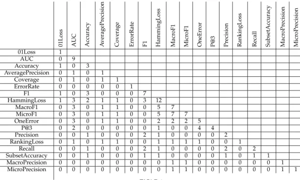
Table 4 shows the occurrences and co-occurrences of the
different measures used in the articles of the corpus C. It
underlines the great variability of the considered criteria, and the frequency distribution allows to distinguish the most popular measures: Hamming Loss (44%), AUC (33%), F1 (26%), Macro-F1 (26%), and Micro-F1 (26%). In addition to these observations, our selection of the suitable measures for the meta-analysis is guided by a recent comparison [154] which has experimentally proved that some measures are highly correlated whereas some others are independent.
More precisely, their authors have tested a set of 16 measures (those present in Table 4 plus some variants) and have compared them with the Pearson and Spearman correlations on 100 000 simulations. Results show that Hamming Loss, Coverage and Ranking Loss are independent, but here only Hamming Loss is taken into account because the frequency
of the two others is very low on C. Results also detect
a strong correlation between the measures of a large set
M = {Subset Accuracy or 01Loss, Accuracy, Precision,
Recall, F1, One Error, Average Precision, Micro Precision, Macro Precision, Micro F1, Macro F1, Micro Recall, Macro
Recall}. Consequently, when several measures of M are
used for a comparison of two algorithms in a same paper, we only retain the most frequent one. Let us precise that AUC and P@3 have not been considered in [154]. But they
have been here added to M as the computation on our
data of their Pearson correlation coefficients with the other
measures ofMconfirms the correlation: its value is ranging
between 0.829 (with Macro-F1) and 0.576 (with One-error) for AUC and is close to 1 (with One-error) for P@3. The two studies with Hamming Loss and the subset of selected
measures fromM(respectively referred to in the following
asHandM) are conducted separately on the article subsets
ofC which take them into account (12 articles forHand 24
forM).
4.1.3 The Consensus Based Approach
Our meta-analysis inspired by the consensus theory [33] [34] is decomposed into two successive steps: (i) filtering the sta-tistically significant domination relationships for the
mea-suresHandM, and (ii) extracting the dominant algorithms
for each measure. Finally we identify the algorithms which statistically dominate the others in the two cases. With a similar process we complete the analysis by distinguishing the algorithms which are dominated.
(a) (b) CCA MLSI MVMD DMLDA MLDA PLST CS SSMDDM HSL LDA
MDDM
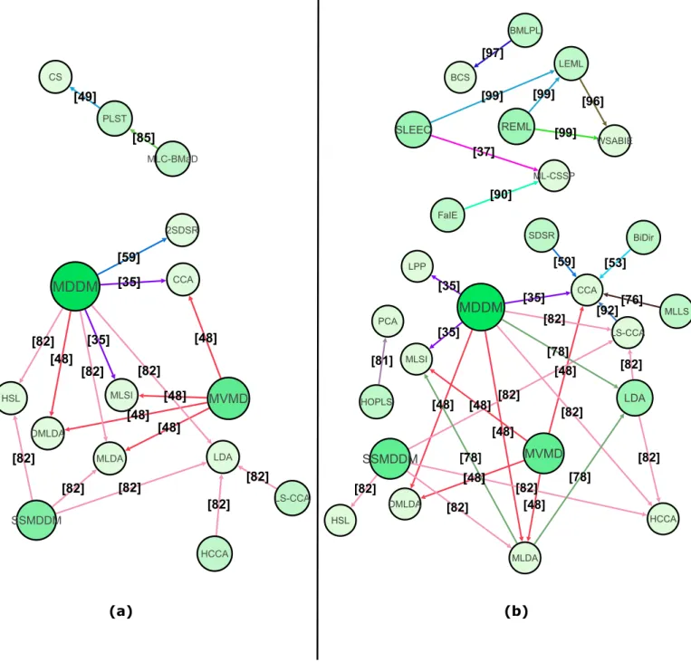
HCCA LS-CCA 2SDSR MLC-BMaD [35] [35] [48] [48] [48] [48] [48] [49] [82] [82] [82] [82] [82] [82] [82] [82] [59] [85] CCA MLSI LPP SLEEC ML-CSSP MVMD DMLDA MLDA BiDir MLLS HOPLS PCA MDDM HCCA LS-CCA SSMDDM HSL LDA FaIE SDSR LEML WSABIE BMLPL BCS REML [35] [35] [35] [37] [48] [48] [48] [48] [48] [48] [53] [76] [81] [82] [82] [82] [82] [82] [82] [82] [82] [92] [90] [59] [96] [97] [99] [99] [99] [78] [78] [78]Fig. 3. Domination multigraphs for Hamming Loss (a) and for the set of correlated measuresM(b). Each directed edge is labeled with the reference of the article from which it is extracted. Different colors are associated to different articles.
More precisely, the significant domination relationships are extracted with a Friedman and post-hoc Nemeyi tests
[155] with a standard confidence level α = 0.05. And, for
each measure, we build a directed domination multigraph
- denoted respectively by GD(H) and GD(M)- from Gc
by retaining the significant edges and by orienting them according to the direction of the domination: a directed edge
from Ai to Aj means that the algorithm Ai significantly
outperforms the algorithmAjin a paper of the corpusC. The
first stage of a topological sorting [156] on each multigraph
allows identifying the subsetsD(H)andD(M)ofAwhich
contains the dominant algorithms: Ai is dominant when
its indegree is null and its outdegree is strictly positive. Similarly, the dominated algorithms are those with a null
outdegree and a strictly positive indegree.
4.2 Results
A multigraph overview reveals communities of algorithms with similar behaviors. A detailed analysis of these commu-nities helps identifying the dominant algorithms.
4.2.1 Algorithm community detection
The two directed multigraphsGD(H)andGD(M)are
rep-resented in Figure 3. They both have a lot less relationships
than the co-occurrence graphGc. With greater alpha
thresh-olds additional directed edges appear but the confidence that can be placed in them is weaker. As a consequence, for
become digraphs with at most one directed edge between
each vertex pairs and some algorithms of A with a null
degree are no more represented. Indeed in some articles the number of experiments is too low to detect a domination which is statistically significant. Table 5 indicates, for each
article ofCand regardless of the considered quality measure,
the ratio CD/rmaxbetween the critical difference CD of the
post-hoc Neymeni test for α = 0.05 and the theoretical
maximal ranking difference rmax between the compared
algorithms. Ifqalgorithms are compared, thenrmax=q−1.
The higher this ratio is, the fewer the expected significant relationships are, and when it is greater than 1 none of them can be extracted.
Ref. CD/rmax Ref. CD/rmax Ref. CD/rmax
[35] 0.613 [79] 0.800 [92] 0.576 [37] 0.754 [81] 0.750 [96] 1 0.462 [48] 0.530 [91] 1.657 [96] 2 1.132 [88] 0.653 [49] 0.800 [97] 0.764 [53] 0.877 [51] 0.693 [99] 1 0.867 [67] 1.386 [82] 0.453 [99] 2 0.676 [68] 1.106 [85] 0.800 [100] 0.828 [73] 0.871 [86] 1.172 [87] 0.778 [76] 0.591 [90] 0.750 [84] 0.762 [78] 0.623 [59] 0.672 TABLE 5
Ratio between the critical difference CD of the post-hoc Neymeni test forα= 0.05and the theoretical maximal ranking differencermax
between the algorithms compared in a given paper. Repeated references are associated to multiple sets of experimental
comparisons.
In the multigraphsGD(H)andGD(M), the communities
identified in sub-section 4.1.1 are associated to different con-nected components: algorithms from different communities have been infrequently compared and are not linked by a significant relationship. Hence, we present the dominant methods for each community. Results are summarized in Table 6. Due to the bibliographic effect which favors the presence of the best approaches at each period, the most recent (resp. oldest) approaches are more likely to be dom-inant (resp. dominated) but there are noticeable exceptions such as MDDM and MLLS.
D(M) D(H)
C1 C1−2 C2 C1 C1−2 C2
MVMD BMLPL MDDM MVMD MLC-BMaD MDDM
SSMDDM REML MLLS SSMDDM
HOPLS SLEEC BiDir LS-CCA
LDA FaIE HCCA
SDSR
TABLE 6
Dominant algorithms detected with the statistical test withα= 0.05for each measureHandMand for each community of the multigraphGc.
Dominant methods for the two measures appear in bold. Different significant thresholds (α= 0.01to0.1) have been tested and, except
for REML forα= 0.01, the highlighted algorithms remain at the top.
4.2.2 In-depth comparison
The three methods (MVMD, SSMDDM and MDDM) that
dominate for both measures belong to communityC1
(label-dependent feature space reduction methods) or toC1−2and
they have close strategies. Let us recall that MDDM mini-mizes the Hilbert Schmidt Independence Criteria between
the reduced feature space and the label space and that MVMD and SSMDDM are hybrid methods whose objective is a trade-off between the objective of MDDM and that of another method (see Table 1a). MVDM and SSMDDM are recent approaches which have been extensively compared to others but in a single paper whereas MDDM, which is older, resists to a larger number of comparisons.
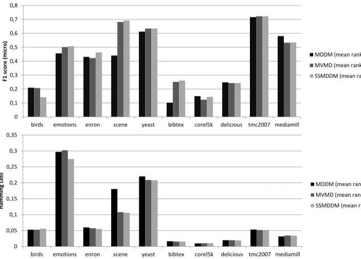
However, to the best of our knowledge, these three meth-ods have not been directly compared to one another. Conse-quently, in an attempt to better understand their behaviors, we have compared them within the same framework. More precisely, the algorithms have been re-implemented (Python language) and tested in the same computational environ-ment (standard computer with 16Gb of RAM). We used ten multi-label datasets often selected in previous multi-label learning studies. They are divided into train/test sets in the
Python library scikit-multilearn2. The feature (resp. label)
dimensionality varies from 72 to 1836 (resp. from 6 to 983).
The reduction methods are combined with the ML-kNN
classifier and the parameter settings are extracted from the
publications. For each method, ten dimensionskxhave been
tested (from 10 to 100 percent of the feature dimensionality
nx) and the best results with the F1-score in the measure
set M and with the Hamming Loss (H) are presented
in Figure 4. With the average rank criterion, SSMDMM outperforms MVDM and MDDM for both measures and
MVDM is better (resp. worse) than MDDM for M (resp.
H). However, when getting into details, we observe that the
results may depend on the datasets: e.g. SSMDMM obtains poor results on the Birds’ dataset. This confirms the interest of the meta-analysis which aggregates results gathered on different experiments involving a variety of datasets. Even if a method outperforms the others on average on a limited number of datasets, it is also worth considering those that do not dominate it in a meta-analysis.
The communityC2is very small inGD(H): the authors
of the algorithms of C2 are mostly interested in data with
a large number of labels and give more importance to ranking measures than to global classification errors such as Hamming Loss. Consequently, there are no methods of
C2simultaneously dominant for the two measures. For the
Mmeasure, SLEEC and REML dominate in several papers.
These methods have been especially designed for extreme multi-label learning, and contrary to the others which build low-rank data representations that can miss the information brought by the long tail label distribution, they compute high-rank representation which capture more useful infor-mation. Due to their efficiency, they have gained popularity in recent years.
In addition to these most visible results, it is interest-ing to identify the approaches that are dominant for one measure and dominated for the other. LS-CCA and HCCA
(resp. LDA) are dominant in GD(H) (resp. GD(M)) and
dominated in GD(M) (resp. GD(H)). These methods are
not intrinsically expected to be more efficient for Hamming
Loss than for the M measures, and due to the absence of
correlation between Mand H, it is not surprising to find
different behaviors. This result confirms the interest of this double analysis.