SEMANTICS ENHANCED DEEP LEARNING MEDICAL TEXT
CLASSIFIER
by
Jose David Posada Aguilar
MS, University of Pittsburgh, 2016
Submitted to the Graduate Faculty of
School of Medicine in partial fulfillment
of the requirements for the degree of
Doctor of Philosophy
University of Pittsburgh
2018
UNIVERSITY OFPITTSBURGH
SCHOOLOF MEDICINE
This dissertation was presented
by
Jose DavidPosada Aguilar
It wasdefended on
July 23, 2018
and approved by
Dr. Harry Hochheiser, Associate Professor, Department of BiomedicalInformatics
Dr. Chakra Chennubhotla, Associate Professor, Department of Computationaland
Systems Biology
Dr. Henk Harkema, Adjunct Assistant Professor, Department of BiomedicalInformatics
DissertationDirector: Dr. Fuchiang(Rich) Tsui, AssociateProfessor, Department of
Copyright c by Jose David Posada Aguilar 2018
SEMANTICS ENHANCED DEEP LEARNING MEDICAL TEXT CLASSIFIER
Jose David Posada Aguilar, PhD
University of Pittsburgh, 2018
Electronic health records (EHR) contain a vast amount of data with the potential to leverage applications that improve patient outcomes and enhance the work of health care providers. A major portion of this data is inside unstructured text in the form of clinical narratives. To effectively use clinical text, NLP tools have been developed and applied to numerous problems involving clinical decision support systems, cohort identification, and phenotyping among others.
However, one of the main problems that face the development of NLP tools for the clinical domain is the lack of large annotated data sets. Clinical language and report style variations are another major problem for clinical NLP. These variations lead to problems where NLP systems created with data from one institution exhibit significantly different performance when tested in a different institution.
One way to address the lack of large annotated datasets and variations in clinical lan-guage is the explicit incorporation of semantics into the development of clinical NLP tools. Semantics allow us to know that the meaning of words, and thus help us account for language variations. In this work, we incorporate the semantics from ontologies into a loss function of a deep learning text classifier. Also, to specifically address the problem of the lack of large annotated datasets we used a large unannotated or unlabeled dataset, increasing the sample size as a result. To properly use such unlabeled data, we adapted a semi-supervised binary approach that uses the unlabeled dataset during training.
To the best of our knowledge we are the first to do so, and for that reason, this is one of the main theoretical contributions of this work. Also, by reducing the need for extensive
annotations, we believe this work could enable researchers in clinical settings to embrace and leverage the full potential of clinical NLP tools given the reduced effort required to achieve the desired performance. Furthermore, all the methods in this work are designed as reproducible and extensible software tools that aid further biomedical informatics research in this area.
TABLE OF CONTENTS PREFACE . . . xi 1.0 INTRODUCTION . . . 1 1.1 THE PROBLEM . . . 2 1.2 THE APPROACH . . . 8 1.2.1 Theses . . . 8
1.3 SIGNIFICANCE AND INNOVATION . . . 10
1.4 THESIS OVERVIEW . . . 11
2.0 BACKGROUND . . . 12
2.1 CLINICAL TEXT CLASSIFICATION . . . 12
2.1.1 Support Vector Machines . . . 12
2.2 DEEP LEARNING FOR NLP . . . 14
2.2.1 Deep Feedforward Networks . . . 15
2.2.2 Word Embeddings . . . 18
2.2.3 Convolutional Neural Networks . . . 21
2.2.4 Long Short Term Memory Networks . . . 23
2.3 DEEP LEARNING TRAINING . . . 24
2.3.1 Loss Functions . . . 25
2.3.2 Regularization . . . 27
2.3.3 Optimization Algorithms . . . 29
2.4 SEMANTIC SIMILARITY IN CLINICAL TEXT . . . 32
3.0 SEMANTICS ENHANCED DEEP LEARNING BASED MEDICAL TEXT
CLASSIFIER . . . 35
3.1 OVERVIEW OF THE METHODS . . . 35
3.2 SEMANTIC DEEP NETWORK . . . 36
3.2.1 Semantic Loss Function . . . 38
3.3 CLASSIFICATION DEEP NETWORK AND TOTAL LOSS FUNCTION 39 3.4 SEMI-SUPERVISED STRATEGY . . . 40
3.5 HYPERPARAMETERS SEARCH . . . 41
3.6 SOCIAL CONTEXT SENTENCE CORPUS FROM PSYCHIATRIC RE-PORTS . . . 42
4.0 EVALUATION . . . 48
4.1 EXPERIMENTS AND METRICS . . . 48
4.2 RESULTS . . . 50
4.2.1 Word Embeddings Training Results . . . 50
4.2.2 Semantic Distance Results . . . 53
4.2.3 Classification Results . . . 57
5.0 DISCUSSION . . . 61
5.1 LIMITATIONS AND FUTURE WORK . . . 64
APPENDIX. CONFIDENCE INTERVALS FOR CLASSIFICATION RESULTS . . . 68
LIST OF TABLES
Table 1. Nonlinear Activation Functions . . . 16
Table2. Social Context Types . . . 44
Table 3. Social Context Sentence Corpus . . . 46
Table 4. Full Set of Experiments . . . 50
Table 5. Example of word2vec closest words . . . 51
Table 6. Examples from Concept Mapping . . . 56
Table 7. Semi-Supervised and Supervised Classification Results . . . 59
LIST OF FIGURES
Figure 1. Psychiatric Report Excerpt . . . 4
Figure 2. Example of an ontology . . . 6
Figure 3. Overview of the Approach . . . 9
Figure 4. Linear SVM . . . 13
Figure 5. Single Neuron . . . 15
Figure 6. Single Layer . . . 17
Figure 7. Deep Feedforward Network . . . 18
Figure 8. Skip-gram model architecture . . . 19
Figure 9. Convolutional Neural Network . . . 22
Figure 10. Long Short-Term Memory . . . 24
Figure 11. Early Stopping . . . 30
Figure 12. Stochastic Gradient Descent . . . 31
Figure 13. Medical Ontology . . . 32
Figure 14. Main Strategy . . . 36
Figure 15. Se-CNN . . . 41
Figure 16. Social context sentence annotation . . . 45
Figure 17. Word2vec Visualization . . . 52
Figure 18. Metamap results . . . 53
Figure 19. Distribution of CUIs in datasets . . . 54
Figure 20. CUI Prevalence . . . 55
Figure 21. Semantic Distance . . . 56
PREFACE
For the LORD gives wisdom; from his mouth come knowledge and understanding
Proverbs 2:6
The fear of the Lord is the beginning of wisdom, and the knowledge of the Holy One is insight.
1.0 INTRODUCTION
Electronic health records (EHR) contain a vast amount of data with the potential to leverage applications that improve patient outcomes, reduce healthcare expenditure and enhance the work of health care providers [1, 2, 3]. It is estimated that roughly 25,000 petabytes of healthcare data will be available by 2020 [1, 3]. A major portion of this data is inside unstructured text in the form of radiology reports, operative notes and discharge summaries among other types of clinical narratives [4]. This clinical text is dictated and transcribed or directly entered by healthcare professionals to communicate the status and history of a single patient to other health care professionals or themselves [5]. This text is what best tells us the patients story and describes the physician thought processes and decision making [6]. Free text continues to be used despite many attempts to encode such information in the form of drop-down menus offered by commercial EHR applications [6].
To effectively use clinical text, natural language processing (NLP) tools have been de-veloped and applied to numerous problems involving clinical decision support systems [4], cohort identification [7, 8], syndromic surveillance systems [9], information extraction [10] and phenotyping [11], among others. Many of these applications depend on some form of text classification. In clinical text classification, the interest is to classify a document into a set of predefined labels that usually represent a disease or condition of interest that is not easily captured by ICD or CPT codes.
Recently, for clinical text classification, deep learning (DL) strategies have gained in-creased attention. Different applications of deep learning applied to clinical text have shown an increase or at least a comparable performance to strategies that rely on handcrafted fea-tures [12, 13, 14, 15, 16, 17, 18, 19, 20, 21]. Usually, these DL text classification strategies rely on pre-trained distributional semantic models for text representation. Distributional
semantic models are models that usually represent word or documents in a vector space. In that space vectors that are close to each other are assumed to have similar meaning, this is being semantically similar. These models are trained with the assumption that words used in similar context have a similar meaning. With that assumption, the models are trained to capture semantics by using the ”distribution” of words in the document.
In consequence, words that rarely occur in a similar context but are related will not be close in the vector space. As an example lets, consider the sentences continued problems in school with frequent suspensions andreceived an undergraduate degree followed by a master’s in Zoology. These sentences are related because both are describing situations related to ed-ucation. However, it is unlikely that the words in the sentences and the sentences itself occur in a similar context within a clinical text. Because of that distributional semantic models will hardly capture the semantic relationship from sentences like those. To overcome this issue, we can supply an external knowledge source containing relationships usually not present on distributional models. Such knowledge source in the biomedical domain is usually presented in the form of ontologies. In the biomedical domain, ontologies have been integrated into DL strategies for word sense disambiguation [22, 23], text classification [24], representation learning for predictive modeling [25, 18]. Outside the biomedical domain, they have been combined for short text classification [26] and to enhance distributional semantic models [27].
1.1 THE PROBLEM
A well-known problem in clinical NLP research is the lack of large annotated data sets. Training samples for clinical NLP are collected through annotation of clinical reports. An-notations are usually performed by clinicians who read through a clinical report and highlight the portion of text that is relevant. Because a clinician performs the task, the cost of an-notating a large corpus is prohibitive for most research projects [28]. That is the reason that when we compare the size of annotated samples for non-clinical text data sets such as bAbI (20,000 samples) [29] or the Imbd movie reviews (50,000 samples) [30], with one of
the most recent annotated clinical data sets (816 samples) [31], we see a notable difference. Any method applied to text classification in the clinical domain needs to account for this problem.
To understand how this problem is solved we need to first describe in more detail the characteristics of those annotations. Clinicians annotate only the portion of text that ex-plicitly contain the relevant information; those annotations are the positive samples. All the other portion of text it is assumed to be non-relevant if the clinician read the entire report, and those annotations become thenegative samples. The majority of the developed clinical NLP exclusively make use of positive and negative samples, requiring fully annotation of the reports. We will name those approaches PN, for positive and negative.
However, if the clinician does not read the entire report, the report is partially annotated, and it cannot be assumed that all the non-annotated text is non-relevant. In this case, those portions of text are considered unlabeled samples because they can be either positive or negative. Unlabeled samples can also be collected through clinical reports the annotator never saw but possibly contain the information we are looking. Partial annotation is done in cases where the time required to read the entire report could prevent the collection of enough samples, or when the annotations are done at a document level or when the information for a given patient in a report is just repetitive and does not contribute to the diversity of the samples. To exemplify this let’s consider the report in Figure 1 and let’s say we would like to annotate information pertaining to living conditions. This particular patient is homeless and the way is described in both of the highlighted sentences is almost the same. Given that the particular living condition for this patient is homelessness, all the information mentioned in the report will be pointing to that. If we want a variety of living conditions, we would have to read a clinical report from a different patient. So instead of spending the precious and costly time of a clinician annotating the same information over and over again, it could be better to ask them to partially annotate this report and move to the next. A report annotated in this form gave way to applications in clinical NLP that only used positive samples [32] or that used a combination of positive, negative and unlabeled samples (PNU) [33, 34]. No attempt has been made in clinical NLP to train a system with only positive and unlabeled samples (PU), and this is one of the focuses of this dissertation.
Figure 1: Psychiatric Report Excerpt. Highlighted in green the relevant information anno-tated
The other major problem with clinical text is that clinical language and clinical report styles vary across institutions [35,36]. Even for the same institution, there is variation across different practices [37]. Prior research shows a significant difference in performance of NLP systems created with data from one institution and tested on data from another [38]. Given this cross-institutional difference it is has been shown that tuning is usually needed when moving a system from one institution to another [39, 40].
One of the ways to address the problem of variability in clinical language and report style is to train with data from multiple institutions [41]. However, this is not always feasible given regulatory restrictions and commercial interests from the healthcare institutions. Another way is to incorporate semantics into the construction of clinical NLP systems [40]. Such semantics can be incorporated through ontologies [42] or distributional semantics models [19]. By incorporating semantics, we can enable NLP systems to understand what is written [43] and consequently improve their performance. As an example, let’s consider the sentences I live by myself, andI live alone. Both sentences are expressing the same reality with different words. An NLP tool trained using only one of the two examples may not generalize well for the second example, without knowing that the meaning of the words by myself and alone is the same in this context.
Several methods have been investigated to incorporate semantics using ontologies. One of the common approaches is to map words or phrases into concepts inside an ontology such as SNOMED [44]. In this approach, instead of using the raw text in a sentence like this he was homeless and living in his car, the mapped equivalent homeless (C0237154), car owner (C0425252)is used to train the models. This approach has been used extensively in different applications that use rule-based [45, 46] or machine learning systems [47, 48, 49, 50, 51]. These studies used the ontological concepts as input features. Most of these applications use a dictionary lookup tool such as cTakes [52], MetaMap [53] or NOBLE Coder [54] to accomplish a mapping.
However, none of these approaches take into account the relationships of those concepts in their ontologies. To account for those relationships some approaches incorporate semantic similarity metrics derived from them. Those similarity metrics are computed by using the hi-erarchical structure of the ontologies, measuring how close two concepts are from each other.
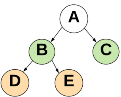
Figure 2: Example of an Ontology
The closeness is measured by accounting for the path between two concepts. Concepts that are closer in the hierarchy (e.g.,D and E in Figure 2) are assumed to be more semantically similar than those that are farther apart (e.g., D and C in Figure 2). One of the ways to incorporate this metric in biomedical text is to use support vector machine (SVM) with a semantic kernel [55, 56, 57]. The semantic kernel is a matrix that contains the concept’s pairwise semantic similarities derived from the ontologies. This matrix is used as the kernel in the SVM. This approach does not take advantage of possibly defining the class as a set of concepts, but keep the class defined as a simple categorical label. This is indeed attempted to solve by [58] where the class is defined as a set of concepts. In this approach, the distance between the set of concepts that form the document and the set that form the class is mea-sured. The document is assigned to the class with lower distance, resembling a k-nearest neighborhood(kNN) approach. In this approach the distance computed does not fully take into account the hierarchy, suffer from the same weaknesses of kNN(e.g., lack of model and computational cost for prediction) and was only applied to biomedical journals but not clin-ical text. In both approaches (i.e., semantic kernel and class-based metrics) semantics that could be derived from the words themselves are not considered, and consequently lost.
Besides ontologies, we can also incorporate semantics through distributional semantic models. Those models are usually trained with unlabeled clinical notes using word2vec [59]
or Glove [60]. Two main approaches have been used to obtain those models. The first one used only the raw text to train such models using simple NLP processes such as tokenization or stop word removal on the raw text [61, 62, 63, 19, 17, 14, 64, 28, 15]. The second use dictionary lookup tool to transform the text into concepts and obtain a model for the mapped concepts [65,66, 13]. Therefore instead of having vector representations for words, the representations are obtained for each concept. In this way, some knowledge from the ontology is transferred by means of word normalization, but the hierarchical relationship of the concepts is lost, and the semantics that could be derived from keeping the raw text representation are also lost.
To overcome this issue, distributional semantic models are improved by using ontologies in a process called retrofitting [67, 27, 68] or by modifying the loss function used to train those models to incorporate knowledge constraints [69,70]. Retrofitting is a process by which those models are modified after training by forcing concepts that are related in the ontology to be related in the models [68, 71]. As an example, let’s assume the vector representation in the distributional semantic model for the words university and midterms are not close to each other. If those words are indeed close in the ontology, the vectors are modified in such a way that the distance between them is reduced. Once these distributional semantic models are obtained, the semantics embedded in those models are leveraged in several works [63,21,12,19,14,15,13] as input features of the machine learning algorithms. However, any of those works merge the representation of the text as concepts, the ontologies hierarchical relationships and the distributional semantics from raw text into the training of the classifiers. A recent work applied to biomedical journals [24], attempts to use the controlled vocab-ulary in the ontology, hierarchical structure, and the distributional semantics. In this work, words that belong to a given group in the ontology share parameters in the model. Groups are formed by merging concepts that share common parents. By merging concepts that share common parents the hierarchical relationships are lost. To illustrate this let’s consider the Figure 2 where according to this approach conceptsB,C andD,E will be merged to groups g1 and g2 respectively. Within those groups model parameters for B, C will be shared but
no sharing will occur betweeng1 andg2 effectively losing the relationship between B and D.
and also focus on the loss function of the classifier rather than enhancing the representation of text, as a markedly different factor from all the previous research that solely focus on modifying the text representation.
1.2 THE APPROACH
We propose a novel approach that combines distributional semantic models with ontologies in a single framework. First, we trained a distributional semantic model from a large corpus of unlabeled clinical reports. The distributional semantic model is in the form of word embeddings. Second, we used an ontology to compute a semantic distance between concepts in the ontology. This distance is incorporated into the loss function of a text classification strategy. The strategy has two main components. The first component is a semantic deep network (SDN) that predicts which concepts are inside a clinical text, similar to the work done by a dictionary lookup tool. The second component is a classification deep network (CDN) that given the probability of each concept in the input text outputs the class label for the text. The unlabeled samples are used in a semi-supervised binary strategy integrated with the SDN and the CDN. The semi-supervised strategy consists of a recursive elimination method that attempts to remove probable positive samples from the unlabeled set of samples. A diagram with the approach is shown in Figure 3.
1.2.1 Theses
In this dissertation, we tested the following hypotheses: (1) the proposed strategy will im-prove the generalization performance of clinical text semi-supervised classification algorithms by incorporating semantics into the training strategy. (2) The proposed strategy will im-prove the generalization performance of clinical text supervised classification algorithms by incorporating semantics into the training strategy
From our experiments, we can conclude the following theses: (1) a semi-supervised clin-ical text classification strategy that integrated a semantic loss function with a recursive
elimination method obtained a better generalization performance than strong clinical text classification baseline methods. (2) Adding a semantic loss function did not improve the gen-eralization performance over strong supervised clinical text classification methods. Based on the experiments performed the following strong claims can be made:
1. Only positive labeled samples are needed to achieve good performance in clinical text classification.
2. To train a semi-supervised strategy that only uses positive and unlabeled samples a non-negative risk loss function is sufficient to evaluate model candidates during hyper-parameter optimization.
3. It is feasible to incorporate prior knowledge into a deep learning strategy in the form of a derivable semantic loss function.
The following weak claim can also be made
• A set based semantic distance function can be directly used to identify probable positive samples to be used for training a clinical NLP tool.
1.3 SIGNIFICANCE AND INNOVATION
To the best of our knowledge, this is the first time that ontologies have been integrated with deep learning to explicitly incorporate semantics into a text classification algorithm applied to clinical text.
Also, to the best of our knowledge, this is the first time that a semi-supervised strategy applied to the classification of clinical text has been trained by only using positive and unlabeled samples. Moreover, our approach is one of the first being applied to a corpus of psychiatric notes.
The principal contribution to informatics is the novelty of hierarchical relationships be-tween ontological concepts to inject semantic relationships into a loss function used to train a text classifier. This process is uniquely integrated into the loss function during classifier training as opposed to preprocessing.
Capturing semantic information reduced the amount of data required to achieve a good level of performance when classifying clinical text. This is advantageous for clinical trans-lational research since the cost and time required to annotate clinical text is prohibitive for most research projects [28]. Our strategy is designed to fill this need, with the pri-mary objective to use less training data. By using less data this work has the potential to enable applications that were restricted for the lack of resources to annotate the number of required clinical reports. Also, applications such as cohort discovery [8] and screening patient’s eligibility in clinical trials from clinical notes [72] can also benefit from this.
Finally, all the methods developed in this work are designed to be reproducible, transpar-ent, accessible and generalizable for future clinical natural language processing applications. We believe this work is important in both biomedical informatics and applied clinical re-search.
1.4 THESIS OVERVIEW
In Chapter 2, a review of the relevant literature regarding clinical natural language pro-cessing, deep learning, and semantic similarity measures in biomedical text is presented. In Chapter 3, all the developed methods are described in detail, along with the development of the dataset used to evaluate the proposed strategy. In Chapter 4, a detailed description of the experiments performed is shown, along with evaluation results on the datasets. Finally, in Chapter 5, a discussion of the results is presented along with the limitations, how to address those and possible future work.
2.0 BACKGROUND
In this chapter, we will discuss relevant concepts regarding clinical text classification, tradi-tional algorithms, and features used for this task. Later we will explain the basic concepts of deep learning pertinent to this work. Finally, we finish with a brief description of semantic similarity measures applied to biomedical text using ontologies.
2.1 CLINICAL TEXT CLASSIFICATION
Text classification is a task that consist in assigning a document to a predefined set of classes or labels [73]. Given an input document d and a set of nC class labels CL ∈ {1, . . . , nC}
we wish to learn a classification function f : d → CL that maps document to classes. For
supervised and semi-supervised learning the class labels are generally known during training, contrary to unsupervised learning where the labels are completely unknown during training. For clinical text, the most common supervised methods are Naive Bayes, support vector machines (SVM), hidden Markov models and conditional random fields [74]. More recently convolutional neural networks (CNN) [21,17] and long short-term memory networks (LSTM) [14] are becoming increasingly popular given their good results in general text. SVM will be described in this section while CNN and LSTM will be described later in Section 2.2.
2.1.1 Support Vector Machines
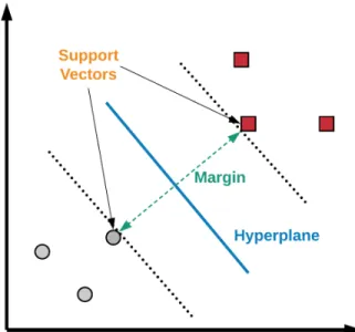
Support vector machines are a binary discriminative learning approach that aims to learn a hyperplane that separates two classes while maximizing the margin between the decision
Figure 4: Linear SVM decision boundary and Margin
boundary. The margin is defined as the distance between the closest data point to the hyperplane that composes the decision boundary between the two classes [73]. Support vectors are called to the data points that are closest to the hyperplane. In Figure 4, we can see an example of a hyperplane, the margin and the support vectors in two dimensions for a linearly separable case.
In general, the decision boundary is non-linear. Thus a nonlinear function is needed to separate the classes. This non-linear function is embedded into SVM in the form of a kernel. The idea of a kernel is to map the input space into a high dimensional space where the data is separable. For this general case, the decision function for a new sample x of an SVM is defined by sign( l X i yiαiK(xi,x) +b) (2.1)
whereK is the kernel function,xi ∈RN, ∀i= 1, . . . , lis the input vector that represents d, with l training samples. yi ∈ {1,−1} are the labels of each class. αi and b are the parameters learn by the algorithm [75,76, 77].
Traditionally to obtain a representation of d suitable for the use with SVM a tf-idf vector space model [78] is obtained from the training corpus. To compute tf-idfvector we need to compute three quantities: the term frequency, the document frequency, and the inverse document frequency. First let’s represent a documentdi in a corpusD as a sequence of words d = (w1, . . . , wn), ∀ di ∈ D. Then we can compute the term frequency tfwj,di as the number of times wj occur in di. Usually, instead of raw counts, we can use a log normalization 1 + log(tfwj,di) to increase the weight of rare words that usually are more informative than common words. Now, to compute the document frequency of a word dfwj we only need to count the number of di that contains wj. The inverse document frequency idfwj is simply the inverse of the document frequency that is usually log scaled and computed by idfwj = 1 +log(l/dfwj). Finally, thetf-idfweight for wj in di can be computed using the equation 2.2.
tf-idfwj,di =tfwj,di ∗idfwj (2.2)
Finally, the input feature vectorxi ∈RN with N as the vocabulary size is formed by the tf-idfweights of each word such that xi
j =tf-idfwj,di.
2.2 DEEP LEARNING ARCHITECTURES FOR NATURAL LANGUAGE
PROCESSING
In the following sections, I describe a neural a network as well as the main architectures used in the present work. I start by describing Deep Feedforward networks (FFN) to later move to word embeddings as an application of this architecture to obtain a distributional semantic model. In Section 2.2.3 I describe convolutional neural networks (CNN) which were initially successfully applied in computer vision applications but has recently gained traction in the NLP community. I then finalize explaining how the networks are trained.
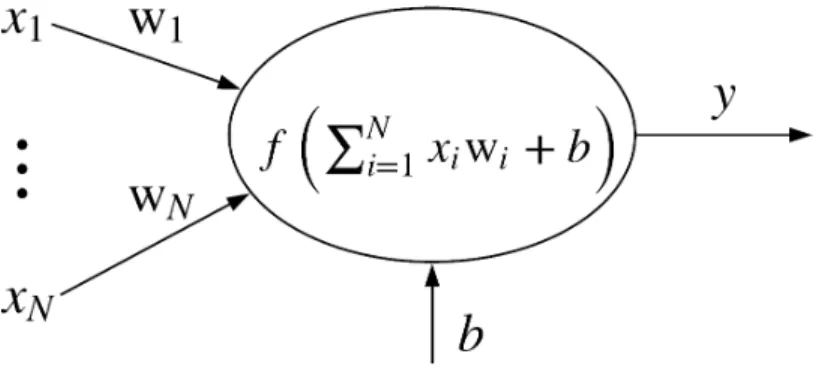
Figure 5: Representation of a basic neuron
2.2.1 Deep Feedforward Networks
Neural networks are a collection of units called neurons that aim to approximate any non-linear function. Originally neural networks are biologically inspired, however in this work we will approach them from the mathematical point of view.
A graphical representation of a basic neuron can be seen in Figure 5. This neuron can be seen as a weighted sum of an input x∈RN with weights w
i ∈ R, ∀ i, . . . , N and a bias term b ∈ R. Here f is a nonlinear activation function applied to the result of the weighted sum.
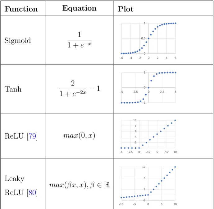
There are several options for nonlinear activation functions. In Table 1 we summarize the most common ones.
A collection of neurons is called a layer. A layer is a collection of neurons that is applied to the same input. In Figure 6, we can see the graphical representation. This layer can be represented in matrix notation as
y=f(xW+b) (2.3)
where W ∈ RN×nout is the weight matrix, and the bias and output are now vectors
b,y∈Rnout.
Now deep feedforward networks (FFN) are typically a composition of multiple of such layers one after another, such that the information flows from the input through the output
Function
Equation
Plot
Sigmoid
1
1 +
e
−xTanh
2
1 +
e
−2x−
1
ReLU [
79
]
max(0, x)
Leaky
ReLU [
80
]
max(βx, x), β
∈
R
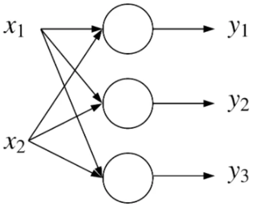
Figure 6: Representation of a basic Neural Network layer with two inputs and three neurons
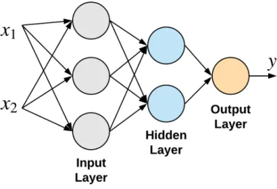
in one direction with no feedback loops or recursion [81] exist. In this networks, there are three main types of layers: an input layer, a hidden layer, and an output layer. An input layer typically is the one that is in direct contact with the input. The hidden layers are the ones that process information as a result of the output of other layers including the input layer. The output layer is the one that produces the final output and is the one where typically the results are observed. In Figure 7, we can see a graphical representation of a prototypical deep feedforward network.
If the classification problem is multi-label multi-class usually a sigmoid function is used in the output layer. In a multi-class problem the classifier is asked to differentiate between a plural number of classes(i.e., more than two). In a multi-label classification problem a clas-sifier is asked to assign more than one label to each sample. On the other hand, if we have a multi-class problem asoftmax function is usually applied to the last layer. softmax normalize the output of the network between zero and one, thus allowing a probabilistic interpretation of the output. For a vectorx∈RN softmax can be defined as:
softmax (x) = PN1 i=1exi ex1 .. . exN (2.4)
Figure 7: Representation of a typical Feedforward network with one input layer, one hidden layer and one output layer
feature representation for text: one-hot, tf-idfand word embeddings. These feature repre-sentations are used as inputs in the first layer of the network. In one-hot representations, each word wj is represented by a0 if it does not occur on documentd and1if it does occur. In this representation, we have a binary feature vector x ∈ ZN with N as the vocabulary size. In tf-idfeach document is represented by a real valued feature vectorx∈RN.
For word embeddings [59] we have a matrix WE ∈ RN×a with a as the size of the embeddings andN the vocabulary size. Here eachwi is represented as a row vector in WE. The vectors for individual words occurring in a document are aggregated using sum, mean or other similar operation [61], to represent a full document. Using this approach the feature vector is x∈Ra. Word embeddings will be discussed in detail in Section 2.2.2.
2.2.2 Word Embeddings
Word embeddings are a distributional semantics representation of words usually obtained through unsupervised training in a large corpus [82]. The most common algorithm to obtain word embeddings is called word2vec [59]. The most common architecture for word2vec is
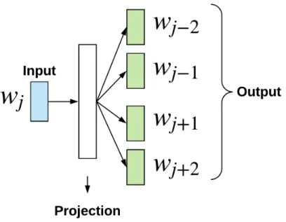
Figure 8: Skip-gram model architecture for word2vec
called Skip-gram (see Figure 8).
In this architecture, the goal is to predict the context words C(wj) = (wj−k, . . . , wj+k) given an input word wj in a window of length k. The model attempts to maximize the average log probability of the corpus D [83]:
arg max
θ
X
(w,cw)∈Dp
log(p(cw|w;θ)) (2.5)
where θ are a set of model parameters, and Dp ⊂ D is a set composed of all word and context pairs that occur in the corpus. Dp is a subset because it is regulated by the size of the context window, so if the context window is infinite, the subset is exactly equal to the set, but this will be computationally intractable. For simplicity, we drop the j index in w, and any word in C(wj) is represented now as cw. The proposed architecture to compute this probability is an FFN with one input layer W ∈ RN×a, one output layer
W0 ∈ Ra×N with softmax output, where a is the size of the embeddings. However, the softmax is not entirely computed but approximated using a method called negative sampling [59]. Negative sampling is a method composed by a mathematical approximation followed
by a series of heuristics where the initial objective proposed in Equation 2.5 is changed by a binary classification problem. In this binary classification problem, the objective is to predict whether a pair of words occur in the corpus or not. In the following, we will describe in detail how the algorithm works.
Letx∈ZN be theone-hotvector representing the wordw. The output of the FFN can be computed asy=softmax(xTWW0),y∈
RN. As we can see from the previous equation, the only non-linearity comes from the computation of the softmax . Computing the softmax is expensive when the vocabulary has millions of words. Instead, the computation is reframed by using rows and column vectors from the input and output weights.
Let vw ∈Ra be a row vector from the matrix W and vcw ∈Ra be a column vector from the matrixW0. Also, let z be a dummy variable that indicates whether a pair (w, cw) is in the corpus or not and defined by:
z = 1 ∀(w, cw)∈ Dp z = 0 ∀(w, cw)∈ D/ p
(2.6)
Now let’s propose two logistic functions to define the probability of z as:
P(z = 1|(w, cw)) =σ(vw·vcw) P(z = 0|(w, cw)) =σ(−vw·vcw)
(2.7)
where σ = 1+exp(−1 x). With this proposition, the new objective is to minimize [83]:
arg max θ X (w,cw)∈Dp logσ(vw·vcw) + X (w,cw)∈D/ p logσ(−vw·vcw) (2.8)
However, to compute the second term, this means the probability for all the samples that do not occur in the corpus will be computationally infeasible. To overcome this instead of computing for all (w, cw) ∈ Dp/ the sum is computed for ns negative samples which become a hyper-parameter of the algorithm. Negative sample pairs are formed such that ((w, cw1), . . . ,(w, cwns)). The objective in Equation 2.8 is more computationally efficient
than a softmax because it is not necessary to obtain the output for each one of theN words in the vocabulary. Instead, this costly procedure is replaced by computing the probability
only for the words in the windowk plusnsnegative samples. To select the negative samples a heuristic is implemented. The heuristic consists in randomly drawing words from the vocabulary with a probability:
pnegative−sample(cwi) =
(tfcwi)3/4
Pns
j=1(tfcwj)3/4
(2.9)
Also, to compensate for too frequent words (e.g. the), each word in a sequence is assigned a probability for keeping such word. If the computed probability is below a predefined thresh-old, the word is discarded. The probability according to their published code is computed by: pkeeping(w) = ( r U(w) 0.001 + 1)· 0.001 U(w) (2.10)
where U(w) is the unigram probability of the word w. Finally, instead of keeping the entire network we only keep the input weights matrix W. That matrix (W) is what we called the embeddings.
2.2.3 Convolutional Neural Networks
Convolutional neural networks (CNN) are neural networks that use aconvolution operation along with matrix multiplication operations to compute their output [81]. A convolution is an operation typical defined in the signal processing world as a real value operation between time-dependent signals. For NLP a convolution is a binary operation that involves segments of text that are represented as real values [84] and a filter or kernel, whose purpose is to extract useful features from the text. One of the advantages of CNN vs. FFN is that we do not need to aggregate the embeddings of words occurring in a document.
To show how embeddings are used with a CNN lets start by defining a document as an ordered sequence of words d = (w1, . . . , wn). Each word is represented as a row vector in WE and thus an input feature matrix x∈Rn×a is formed by the concatenation of each row vector that represents each wj. Next, a convolution filter is applied to the feature matrix. A convolution filter is defined as a matrix of weights W ∈ Rh×a where h <= n is the size of the sliding window in which the convolution is applied. Before defining the convolution,
Figure 9: Convolutional Neural Network with Word Embeddings
let us define first the concatenation of h consecutive row vectors as xj:j+h−1. Then we can
define the result of the convolution ck∈R as:
ck=f(W·xk:k+h−1 +b), ∀ k = 1, . . . , n−h (2.11)
where · is the dot product, b ∈ R is a bias term, and f is a nonlinear function (see Section 2.2.1). After doing the convolution over the entire document we have a feature map
cW = [c1, . . . , cn−h] ∈ Rn−h [85]. Over this feature map we apply a max-pooling operation ˆ
cW = max (cW),cˆW ∈R[86]. Given that we can have multipleqfiltersW ={W1, . . . ,Wq} we can form a feature pooled vectorˆcW = [ˆcW1, . . . ,ˆcWq],ˆcW ∈ Rq [84]. After this, we use an FFN with at least one layer withˆcW as the input and y∈RnC as the output vector for nC class labels. Without hidden layers, we will have a weight matrix WFFN ∈ Rq×nC. The final output is obtained by using asoftmax function overy. A graphical representation of a CNN for NLP can be seen in Figure 9.
2.2.4 Long Short Term Memory Networks
Long short-term memory networks (LSTM) are a type of recurrent neural networks (RNN) were the order of the input sequence is taken into account. To make predictions the input sequence does not need to have a fixed length [82]. Specifically, an LSTM was designed to address the vanishing gradient problem with long-term dependencies, allowing predictions with longer sequences than a regular RNN [87]. An RNN is called recurrent because part of their output is feedback to the input. As well as CNN, LSTM can use the word embeddings directly without the need for an aggregation operator.
In an LSTM there are five main components which can be defined as vectors in Rhu: an input gate ij, an output gate oj, a forget gate fj, a cell state cj, and an output state hj. In all of those vectors hu represent the number of hidden units. The input of this network is again a feature matrix x ∈ Rn×a produced as the concatenation of the row vectors from the word embeddings that represent the document d. xj, ∀ j = 1, . . . , n is a single row in the feature matrix representing the wordwj in the ordered sequence. Also, we will represent the concatenation of two row vectors with [ ;]. The graphical representation of the required computation for an LSTM is shown in Figure 10. To compute the output hj we need the following equations [82, 14] oj =σ(Wioxj +bio+Whohj−1+bho) ij =σ h Wii(xj) T +bii+Whihj−1+bhi i gj = tanh(Wigxj +big +Whchj−1+bhg) fj =σ(Wifxj+bif +Whfhj−1+bhf) cj =fjcj−1+ij gj hj =oj tanh(cj) (2.12) Wii,Wif,Wig,Wio ∈Rhu×a Whi,Whf,Whc,Who ∈Rhu×hu bii,bhi,bif,bhf,big,bhg,bio,bho ∈Rhu σ :sigmoid,: component wise product
Figure 10: Long Short-Term Memory Network with Word Embeddings
All the gates outputs are computed by using the previous output state hj−1 and the
current input xj. hj−1 is also used to update candidate gj. The forget gate fj controls how much of the previous cell state cj−1 is considered to compute the new cell state cj, and the input cell ij controls how much of the proposed update to keep. Finally, the output gate
oj controls how much of the current state cj is used to compute the output state hj. To compute a final output we could usehn directly or use this output state in combination with an FFN layer and softmax or sigmoid output.
2.3 DEEP LEARNING TRAINING
To train a neural network, we need to usually specify three main things: the architecture, the loss function, and the training algorithm. We will go over each one of them in the following sections.
2.3.1 Loss Functions
Loss functions are an essential component of the training since they specify how good a given classifier is doing. They define what is good and what is bad, so for a given dataset, they are the eyes that look at how well the strategy is doing. The two most common loss functions used in neural network training for NLP are Hinge and cross entropy loss. These losses are computed for each training samplej using the predicted output ˆyi ∈RnC and the true outputyi ∈RnC wherenC is the number of classes. Let us represent a loss function as L(ˆyi,yi)∈ R and the total loss for all the samples is usually computed as the sum of each of the sample loss:
LT = l X
i=1
L(ˆyi,yi) (2.13)
Usually, the loss should be zero if a perfect classification was made. Now, we will show explicitly how the different losses are computed. Without loss of generality, in the following equations, we will drop the sample index i to simplify the equations when possible.
Hinge Loss
For binary classification problems, the output of the network is usually a scalar ˆy ∈ R and the class labelsy∈ {−1,1}. This is similar to what is done in an SVM and, like in that case, the decision function is sign(ˆy). A correct classification is produced if y∗y >ˆ 0. Is important to consider that the output for the network when using this loss function is usually between (−∞,+∞) and linear. Finally, for a single sample the loss can be formulated as [82]:
LHinge(ˆy, y) = max (0,1−y∗y)ˆ (2.14)
This loss attempts to have a correct classification with a margin of at least one
Multiclass Hinge Loss
The multiclass extension of the hinge loss was proposed by [88] where now ˆy ∈ RnC is the predicted output vector, and the true class labels are a one-hot vector y ∈ RnC. It is important to notice that here the output is not a probability but a score that in general is
not bounded. To classify a sample, we need to compute:
prediction= arg max(ˆy) (2.15)
The loss can be computed in two ways. The first one [82] only considers the prediction for the highest scoring class as shown in the following equation:
LHinge(ˆy,y) =
max (0,yˆj−yˆk+ ∆) if arg max(ˆy)6= arg max(y)
0 otherwise
(2.16)
where ˆyj = max(ˆy) and ˆyk is the output for the true class with k = arg max(y) being the index for the true class. This loss function wants the predicted score for the correct class being larger than the score for any other class at least for a margin ∆. Classically, this margin is static and have the value of one, but in general is a hyperparameter to be tuned.
The second way is to consider all the other scores for all the other classes into the computation of the loss, thus this time attempting to produce not just a high score for the true class but the lowest possible score for all the other classes that are not the true one. This function can be defined as:
LHinge(ˆy,y) = X j max (0,yˆj −yˆk+ ∆) (2.17) ˆ yj ∈yˆ, ∀j(j ∈ {1, . . . , nC} ∧j 6=k), k = arg max(y)
The first one is more appealing since a prediction is not needed for all the classes and only for the one that has the maximum predicted value.
Cross Entropy Loss
When the outputs of the neural network can be interpreted as probabilities a cross entropy loss can be used. The output of the network is usually normalized using a softmax , and in consequence, we could interpret such output as a probability of each class. This time let
y={y1, . . . , ynC} be set representing the true multinomial distribution over nC classes and
let ˆy = {ˆy1, . . . ,yˆnC} be the network’s output. Because we are using softmax , the output can be interpreted as ˆyj =P(yj|x) where xis the input of the network. Thus, the categorical
cross entropy is measuring the dissimilarity between the two probability distribution and is defined as: LcE = (ˆy,y) = − X j yjlog ˆyj (2.18) 2.3.2 Regularization
Usually to avoid overfitting several strategies need to be used for training a deep neural network. Due to the vast amount of parameters, the network can easily overfit the training data and perform poorly on unseen data. Three types of regularization methods are discussed in this section. The first one imposes penalties on the learned weights, the second attempts to regularize the intermediate layer outputs, and the third one uses a developing set to stop the training process.
Parameter Norm Penalties
In this family of regularization, the two most used methods are L1 andL2 regularization
[81]. Both methods impose an additional term to the loss function that depends exclusively on the norm of the weights. With this regularization a loss function takes the following form:
LT = l X
i=1
L(ˆyi,yi) +αΩ(θ) (2.19)
whereθis the set of model parameters andα∈[0,∞) is a hyperparameter that regulates the contribution of the penalty term to the total loss function. In L1 regularization Ω(θ) is
substituted by the L1 norm. In the L2 regularization Ω(θ) is substituted by L2 norm. Each
of the norms is computed by:
L1 =kθk1 =|W| (2.20) L2 = 1 2kθk2 = 1 2W TW (2.21)
where W are the weights of each one of the layers.
Layer’s Output Regularization
For layer’s output regularization two main techniques are presented here: dropout [89] and batch normalization [90]. Dropout is a technique that randomly drops components of the input vector of any layer using a Bernoulli distribution. Formally let x ∈ RN be an input vector and a random vector r∼Bernoulli(pr),r∈RN with probability pr, a dropout operation is defined as:
˜
x= 1
1−prxr (2.22)
where is the component-wise product and ˜x is the vector used now as the input for the layer. During test time r is not generated and thus ˜x=x. This technique attempts to prevent co-adaptation by relying only on some specific weights to produce an output. In [91] is shown that dropout has a strong connection with L2 regularization.
The second technique, batch normalization, attempts to reduce the amount of change in the distribution of network activations. This change is called internal covariate shift. Through the use of batch normalization, the optimizer is less likely to get stuck in saturated regime and training would accelerate [90]. Let xij ∈ xi be the values of the variable j in sample i. Let us define a batch for a variable j as a series of consecutive m samples as Bj ={x1j, . . . , xmj}. First, to compute the normalized output for the variable j x˜ij we need to compute the mean and variance of the batch as
µBj = 1 m m P i=1 xij σ2 Bj = 1 m m P i=1 xij −µBj (2.23)
then we standardize the input
ˆ xij = xij −µBj q σ2 Bj+ (2.24)
where is a constant added for numeric stability. To finally produce the output:
˜
xij =γxˆij +β, ∀ γ, β ∈R (2.25)
where γ and β are parameters to be estimated. As we can see, batch normalization becomes another layer of the neural network. At test time, means and the variances estimated during training are used for testing. In consequence, γ, β, µBj, σ
2
Bj are constants during testing.
Early Stopping
Early stopping is a regularization technique that stops the training process before the overfitting happens [81]. For this technique, a separate developing set is required. This developing set is used to compute the same loss being optimized or another relevant perfor-mance metric to the task (e.g., precision). Using the result of this computation a decision is taken to whether continue training or stop. The decision is taken in two different ways. The first one is checking if the validation loss is going up instead of going down. The second is checking if the validation loss is not changing at all. For both strategies two parameters are defined: patience and δ∈ R. Patience is the number of iterations/epochs to wait while the condition is met before to stop training. δ is the threshold used to decide whether a change in the metric being watched is taken into account or not. In Figure 11 a flowchart with the strategy is shown. The meaning of epochs and iterations is clarified in the Section 2.3.3.
2.3.3 Optimization Algorithms
Stochastic gradient descent (SGD) and their variants are the most widely used algorithms for deep learning training [81]. Stochastic gradient descent is a modification of the original gradient descent [92, 93]. The most significant difference of SDG vs. traditional gradient descent in the use of the batch B (sometimes referred as minibatch). The batch is no more than a set composed by a sample of the training data. Rather than computing the gradient after passing all the data through the network, SGD computes the gradient and modify the weights by only using the batch (see Figure 12). The batch size|B|is usually greater than one and less than the training sample size. However, smaller sizes are currently preferred since
Figure 11: Early Stopping using a Validation Set. Other stopping criteria includes number of epochs, number of iterations and minimum required loss.
Figure 12: Stochastic Gradient Descent Algorithm with batches
they produce faster convergence [82]. They also improve training efficiency by computing the steps in lines 3 and 4 of Figure 12 in parallel. Given that now with have batches anepoch is defined as the moment where all the training data has been used for modifying the weights in the network. In consequence, an epoch is composed of several iterations. If the sample taken from the batch is without replacement, we can compute the number of iterations as bl/|B|c where l is the number of samples, and b/c is the integer division. If the division is not exact, there are two possible options. In the first option, the last batch is bigger. In the second the samples in the last batch are discarded. To compute the gradient several automatic differentiation techniques have been proposed [94], and they are currently used by popular frameworks such as TensorFlow [95] and PyTorch [94]. The later is the one being used in the present work. Those techniques allow the computation of the gradient without the need to define it explicitly. The only requirement is that the loss function must always be positive and differentiable.
Figure 13: Snapshot of SNOMED CT Ontology. Path between two concepts (blue). For this case the path has a value of five. In green, we can see the least common subsummer of the two highlighted concepts
2.4 SEMANTIC SIMILARITY IN CLINICAL TEXT
Semantic similarity is a metric of how similar are the meanings of two words. This similarity can be measured using distributional methods or ontologies. With distributional methods, we rely on the hypothesis that words occurring in the same context tend to have the same meaning [96]. With ontologies, we rely on the taxonomic structure to define the similarity [97]. In ontologies word of phrases are seen as concepts. This has the advantage that ontologies can be used as a source for word normalization or as a controlled terminology. Those concepts have relationships to other concepts as part of the definition of the ontology. One of those relationships ins the is-a relationship that define a hierarchy between the given concepts, e.g., Failed Exams is-a Academic Problem. In the biomedical domain, other useful relationships are part-of and treated-by. In the present work, we will limit to the is-a relationship. In the following, metrics to measure the semantic similarity between two concepts in an ontology are presented.
2.4.1 Semantic Similarity using Ontologies
An ontologyOis a set of conceptscithat belong to a controlled terminology usually organized in a tree-like structure (see Figure 13). The simplest way to compute the semantic similarity between two concepts in the ontology is using the pathpbetween them. The path is defined as the shortest path between two concepts in the tree as seen in Figure 13. Thus, the similarity between two conceptsc1 and c2 is defined by [98]:
simpath(c1,c2) =
1
p (2.26)
However, the main drawback of this measure is that does not take into account how big is the ontology. Tho address this issue a new measure was proposed [99] and later normalized to the unit scale [100]. This measure is usually called LCH because of the authors Leacock & Chodorow. The following equation defines the metric:
simLCH(c1,c2) = 1−
logp
log 2d (2.27)
whered is the maximum number of nodes from the root to any concept. Later on, a new metric was proposed [101] to take into account the granularity of the least common subsumer of two concepts lcs(c1,c2). lcs is the closest common parent of any two given concepts (see
Figure 13). The normalized version as available in the NLTK Toolkit [102] is:
simwp(c1,c2) =
2∗depth(lcs(c1,c2))
p−1 + 2∗depth(lcs(c1,c2))
(2.28)
where the depth of a concept is the number of nodes in the path between the root and the concept. Besides paths, we can also use the information content IC(ci) to measure the semantic similarity. This metric attempts to quantify information by measuring a ratio between the number ofleaves and the number of subsumers. Theleaves are a set formed by the descendants of a concept that have no descendants. The subsumers is a set formed by all the ancestors of a concept included the concept itself. The information content is defined
by [103]: IC(ci) = −log |leaves(ci)| |subsumers(ci)| + 1 maxLeaves+ 1 (2.29)
where maxLeaves is the total number of leaves in the ontology. Using this metric, we can measure the semantic similarity between two concepts by [100]:
simLIN(c1,c2) = 2∗IC(lcs(c1,c2)) IC(c1) +IC(c2) (2.30)
3.0 SEMANTICS ENHANCED DEEP LEARNING BASED MEDICAL TEXT CLASSIFIER
In this dissertation, we developed a supervised and semi-supervised deep learning strategy. Our strategy aims to classify clinical text incorporating a semantic similarity loss as part of the training process. A corpus of social context sentences inside psychiatric reports was used to assess the performance of the proposed strategy. The main contributions of the proposed strategy are: (1) incorporate a medical ontology as prior knowledge into a deep learning strategy, (2) train a deep learning strategy using such ontology to compute a semantic loss that is used during training, (3) use unlabeled data during semi-supervised training.
3.1 OVERVIEW OF THE METHODS
Deep knowledge-based Semantics Medical Text Classifier is a deep learning strategy for classifying medical text that is composed of two components: a semantic deep network (SDN) and a classification deep network (CDN). The primary task of the SDN is to predict the most probable concepts present in the text. The CDN uses the prediction from SDN to assign the most probable label to the input text. Formally, given a tokenized input document d and a set of nC class labels CL∈ {1, . . . , nC}, the strategy will predictP(CL|d).
Both networks are trained simultaneously by backpropagation using a loss function that incorporates a semantic loss and a classification loss. The semantic loss function is computed using the output from SDN and a medical ontology (e.g., SNOMED). For the classification loss, we used cross-entropy or a modified hinge loss. Both losses are described in Section 2.3. Details of both networks and how the losses are computed are given in the following
Figure 14: Overall design of the deep learning strategy
sections. In Figure 14, we can see a graphical representation of the strategy.
3.2 SEMANTIC DEEP NETWORK
Given a tokenized input document d as an ordered sequence of n words wi such that d = (w1, . . . , wn) the task of SDN is to predict the most probable m (m <= n) set of concepts SC ={c1, . . . ,cj, . . . ,cm, ∀ cj ∈ O} inside d, with O as the ontology. More formally, given d, SDN predicts P(SC =cj|d), ∀ cj ∈ SC.
SDN will have two possible architectures CNN and LSTM (see Section 2.2). For both architectures, the first component is the word embeddings. For embeddings constructed with algorithms that consider only entire with words(e.g., word2Vec [59]) they are represented as
WE∈RN×a whereN is the size of the Vocabulary V, and a is the size of the embeddings.
WEtransformdinto feature matrixx∈Rn×a. In the following, the result of the embedding operation over d will be represented as x∈Rn×a.
As the output of this network regardless of which architecture is used asigmoidactivation function is used in the output layer. Thesigmoidfunction has some desirable properties such as bounded output (0,1) and smooth gradient. If we interpret each output as a probability they are mutually exclusive, so in general they not sum up to 1, because d can contain multiple concepts. Each node in the output represents a concept in the ontology, and it is assigned before the training process starts and its keep consistent during all training and evaluation.
However, the issue that emerges here is that the number of possible concepts to predict is the combination |O|l
. To give an example, an ontology such as SNOMED has more than 3×10⁵ concepts, if we consider only 1000 and a sequence of length 10 we have 2.63×10²³ possible predictions. To solve this problem, we will only consider the top k outputs using k-max pooling [104]. Formally, given a predefined value k and a sequence p ∈ Rp where p≥k, k-max pooling selects a subsequence pk
max of thek highest values of p [104]. For the rest of the values, a zero is assigned to nullify the effects of further operations that feed on those nodes. This is similar to what occurs in a dropout layer. In consequence, we can then represent the output of SDN as ˆySDN ∈Rk after the k-max pooling layer.
The next aspect to consider is how this network is trained. Given that the input is a sequence of words, initially, we do not have the actual concepts that occur within the sequence. To solve this problem I used MetaMap [53] to obtain SC and use those are labels. The output of MetaMap is only used in conjunction with the loss function in Equation 3.4. Now given a set of mapped concepts SC, we formulated a supervised loss function using a structured hinge loss [105] as
LHingeSDN =max(0, s(SC|x)−s(SCtrue|x) +SL(ˆySDN)) (3.1)
Where SL is the semantic loss. The computation of SL is explained in detail in Section
3.2.1. In this equations(SCtrue|x) is computed for the set of true concepts regardless of they being the top k and s(SC|x) is computed for the top k obtained after the k-max pooling layer.
In general the score s is computed as s(SC|x) = k X j=1 ˆ ySDNj = k X j=1 P(SC=cj|x) (3.2)
3.2.1 Semantic Loss Function
In this function, we wanted to capture how semantically similar is an input document to a target class defined as a set of concepts in an ontology. We wanted this loss function to have a [0,1] range. This loss is defined as an inverse measure of a semantic similarity because we want the most similar elements to have zero loss. With this bounded range, it resembles a distance function. In the following, we will treat this loss as a distance function.
A target class is usually defined as an integer label which does not adequately represent everything that a class comprises. Here we attempt to extend the definition of a target class. In this work we defined a target class as a set of concepts in an ontology. Formally let us represent a target class as CO ⊂ O. The elements in CO are selected by an expert clinician
and should represent his knowledge about a particular condition of interest. In this work, we limit the expressiveness to a set of concepts without further using first-order logic (FOL). By doing this, we exclude properties on the concepts such as negation.
Given CO and SC, we used a distance [106] that takes into account the hierarchy of the
ontology. The loss can be computed using the following equation:
SL(ˆySDN) = 1 |SC ∪ CO| X cj∈SC\CO 1 |CO| X ci∈CO d(ci,cj) + X ci∈CO\SC 1 |SC| X cj∈SC d(ci,cj) (3.3)
Here d(ci,cj) is the distance between two concepts which is computed using the metric presented in equation 2.30.
Incorporating the hierarchy in the semantic loss is used to inform about similarities that otherwise may be hindered. Let’s use as an example the following sentencesshe will now not be able to go to college, and She did not graduate from special education at the high school level. The mapped concepts from those sentences are[College (C0557806), Able (C1299581)], and [Special Education (C0013649), High School Level (C0683862)]. If we use a metric such
as the Jaccard distance, that does not take into account the hierarchy, there is no similarity between those sentences because they do not share common concepts. The concepts in both texts are different, but it is obvious that they are talking about academic problems. What is needed to know this is a hierarchy that reflects this similarity, because without them there is no relationship between those sentences because there is no intersection. So this semantic loss is not directly aiding the prediction of the concepts made by the SDN but the classification task by informing about similarities in the input text.
3.3 CLASSIFICATION DEEP NETWORK AND TOTAL LOSS FUNCTION
Given the output of the SDN as ˆySDN the classification network implements a non-linear function f :Rk →
RnC to classify the input text in one of eachnC classes. The architecture for this network is a Feed Forward Network as described in Section 2.2.1. The output of this network is a softmax .
For training, we proposed two functions: an additive loss and a hinge loss. The additive loss is computed using the following equation:
Ladd=LcE(ˆyCDN,y) +λ∗LHingeSDN (3.4) where LcE is the cross-entropy loss (Equation 2.18), λ is a scalar, ˆyCDN is the predicted output and yis the true output. The hinge loss is defined by:
LHinge =max(0, s(ˆyCDN|x)−s(y|x) +SL(ˆySDN)) (3.5)
where s(ˆyCDN|x) is the score for the output with the maximum predicted value and s(y|x) is the score for the predicted true output. In this case, the score is the unnormalized output of CDN. As an example, let us say we have two outputs and the true label is 1. If the output of the network is [10,20] the maximum value is in index 2. In this case, the predicted score is 20, and the score for the correct output is 10. The scores can be computed using the unnormalized output of the network. This means the score is computed before applying the softmax .
3.4 SEMI-SUPERVISED STRATEGY
To use unlabeled samples to improve generalization we used to three methods. The first one was training word embeddings using the method described in Section 2.2.2. The second has to do with hyperparameters search and will be explained in Section 3.5. The third is presented in this section, and it is a strategy that directly deals with unlabeled samples while training a text classifier. The semi-supervised strategy we used belongs to a subset of binary classification strategies called positive and unlabeled (PU) learning [107]. In this mode of learning, we have two sets available for training: positive and unlabeled. The positive set contains samples adequately labeled as belonging to a class of interest. The unlabeled set contains samples that could be either positives or negatives. By negatives, we mean samples that do not belong to the class of interest. To evaluate the overall performance of the strategy a small subset of positive and negative samples are usually obtained.
In this work, we modified a recently proposed strategy [108] for PU learning that uses text data. In this strategy, an iterative process is proposed where probable positive samples are removed from the unlabeled set. In the previous work, they used an FFN in combination with part of speech tags to make predictions for single words. In this work, we used a CNN and the proposed strategy as the classifiers. The algorithm for the strategy is shown in Figure 15.
In step 5 a binary CNN is trained or a binary version of the proposed strategy. The threshold in step 8 is computed by assuming a Gaussian distribution of the predicted proba-bilities for the spy samples. Thusφis computed by using the maximum likelihood estimation of the mean µand the standard deviation sd as shown in the following equations:
φ =µ+ sd µ= 1 |S| |S| P i=1 sSi sd = 1 |S| |S| P i=1 (sSi−µ) 2 !1/2 (3.6)
Figure 15: Spy-based elimination of positive class instances using CNN
3.5 HYPERPARAMETERS SEARCH
Given the extreme importance of the hyperparameters in the performance of deep learn-ing strategies [109, 110, 111] we performed a random search [110] to find the best set of hyperparameters using the developing set.
For the Binary dataset, we used the F1 score as the criteria to maximize given a set
of hyperparameters. However, for the PU dataset, the true negatives are unknown during training. For this reason, a loss or a risk function is needed to guide the search by only using positive and unlabeled examples. Recently a non-negative risk estimator for positive and unlabeled learning (NNPU) was developed [112]. This risk guarantees a reduction in the mean squared error. We selected the hyperparameters with the minimum risk. The risk can
be estimated using the following equation: e Rpu(g) =πpRb+p(g) + max n 0,Rb − u(g)−πpRb − p(g) o . (3.7)
In this equationπpis the positive class prior or prevalence, andRb+p(g),Rb−u(g), andRb−p(g) can be estimated by:
b R+p(g) = 1 np np X i=1 `(g(xpi),+1) (3.8) b R−u(g) = 1 nu nu X i=1 `(g(xui),−1) (3.9) b R−p(g) = 1 np np X i=1 `(g(xpi),−1) (3.10) Herexpi and xu
i are the positive and unlabeled input samples respectively, g is a decision function for binary classification. In other words, g is the function that applies out proposed text classifier to the input feature vector. Finally, `: R× {±1} → R is a loss function that for our case is a sigmoid of the form
`sig(y, t) =
1
1 + exp(yt) (3.11)
where y= 2∗arg max(ˆyCDN)−1 and t= 2∗arg max(y)−1. These transformations are done because those equations need an -1/1 type output.
3.6 SOCIAL CONTEXT SENTENCE CORPUS FROM PSYCHIATRIC
REPORTS
To assess the performance of the proposed strategy we used a previously created corpus of social context sentences from psychiatric reports. The goal of this corpus is to train text classifiers capable of classifying sentences in psychiatric reports that contain social context information. To create this corpus, we developed the description for social context using